Sampleable Functions Based on Codes
?Thomas Debris-Alazard1,2, Nicolas Sendrier2, and Jean-Pierre Tillich2
1
Sorbonne Universit´es, UPMC Univ Paris 06 2
Inria, Paris
{thomas.debris,nicolas.sendrier,jean-pierre.tillich}@inria.fr
Abstract. We present here a new family of trapdoor one-way functions that are Preim-age Sampleable on AverPreim-age (PSA) based on codes, the Wave-PSA family. The trapdoor function is one-way under two computational assumptions: the hardness of generic decod-ing for high weights and the indistdecod-inguishability of generalized (U, U+V)-codes. Our proof follows the GPV strategy [GPV08]. By including rejection sampling, we ensure the proper distribution for the trapdoor inverse output. The domain sampling property of our family is ensured by using and proving a variant of the left-over hash lemma. We instantiate the new Wave-PSA family with ternary generalized (U, U+V)-codes to design a “hash-and-sign” signature scheme which achieves existential unforgeability under adaptive chosen message attacks(EUF-CMA) in the random oracle model. For 128 bits of classical security, signature sizes are in the order of 13 thousand bits, the public key size in the order of 3 megabytes, and the rejection rate is below one rejection every 100 signatures.
Code-Based Signature Schemes. It is a long standing open problem to build an efficient and secure digital signature scheme based on the hardness of decoding a linear code which could compete with widespread schemes like DSA or RSA. Those signature schemes are well known to be broken by quantum computers and code-based schemes could indeed provide a valid quantum resistant replacement. A first answer to this question was given by the CFS scheme proposed in [CFS01]. It consisted in finding parity-check matrices H ∈ Fr2×n such that the solution e of smallest weight of the equation
eH|=s. (1)
could be found for a non-negligible proportion of all s in Fr
2. This task was achieved by using high rate Goppa codes. This signature scheme has however two drawbacks: (i) for high rates Goppa codes the indistinguishability assumption used in its security proof has been invalidated in [FGO+11], (ii) security scales only weakly superpolynomially in the keysize for polynomial time signature generation. A crude extrapolation of parallel CFS [Fin10] and its implementations [LS12, BCS13] yields for 128 bits of classical security a public key size of several gigabytes and a signature time of several seconds. Those figures even grow to terabytes and hours for quantum-safe security levels, making the scheme unpractical.
This scheme was followed by other proposals using other code families such as for instance [BBC+13, GSJB14, LKLN17]. All of them were broken, see for instance [PT16, MP16]. Other signature schemes based on codes were also given in the literature such as for instance the KKS scheme [KKS97, KKS05], its variants [BMS11, GS12] or the RaCoSS proposal [FRX+17] to the NIST. But they can be considered at best to be one-time signature schemes and great care has to be taken to choose the parameters of these schemes in the light of the attacks given in [COV07, OT11, HBPL18]. Finally, another possibility is to use the Fiat-Shamir heuristic. For instance by turning the Stern zero-knowledge authentication scheme [Ste93] into a signature scheme but this leads to rather large signature lengths (hundred(s) of kilobits). There has been some recent progress in this area for another metric, namely the rank metric. A hash and sign signature scheme was proposed, RankSign [GRSZ14], that enjoys remarkably small key sizes, but it got broken too ?This work was supported by the ANR CBCRYPT project, grant ANR-17-CE39-0007 of the French
in [DT18]. On the other hand, following the Schnorr-Lyubashevsky [Lyu09a] approach, a new scheme was recently proposed, namely Durandal [ABG+18]. This scheme enjoys small key sizes and managed to meet the challenge of adapting the Lyubashevsky [Lyu09b] approach for code-based cryptography. However, there is a lack of genericity in its security reduction, the security of Durandal is reduced to a rather convoluted problem, namely PSSI+ (see [ABG+18, §4.1]), capturing the problem of using possibly information leakage in the signatures to break the secret key. This is due to the fact that it is not proven in their scheme that their signatures do not leak information.
One-Way Preimage Sampleable Trapdoor Functions. There is a very powerful tool for building a hash-and-sign signature scheme. It is based on the notion ofone-way trapdoor preim-age sampleable function [GPV08, §5.3]. Roughly speaking, this is a family of trapdoor one-way functions (fa)a such that with overwhelming probability over the choice offa (i) the distribution of the images fa(e) is very close to the uniform distribution over its range (ii) the distribution of the output of the trapdoor algorithm inverting fa samples from all possible preimages in an appropriate way. This trapdoor inversion algorithm should namely sample for anyxin the output domain offa its outputsesuch that the distribution ofeis indistinguishable in a statistical sense from the input distribution to fa conditioned on fa(e) = x. This notion and its lattice-based instantiation allowed in [GPV08] to give a full-domain hash (FDH) signature scheme with a tight security reduction based on lattice assumptions, namely that the Short Integer Solution (SIS) problem is hard on average. Furthermore, this approach also allowed to build the first identity based encryption scheme that could be resistant to a quantum computer. We will call in this paper, this approach for obtaining a FDH scheme, the GPV strategy (the authors of [GPV08] are namely Gentry, Peikert and Vaikuntanathan). This strategy has also been adopted in Falcon [FHK+17], a lattice based signature submission to the NIST call for post-quantum cryptographic primitives that was recently selected as a second round candidate.
This preimage sampleable primitive is notoriously difficult to obtain when the functionsfa are not trapdoor permutations but many-to-one functions. This is typically the case when one wishes quantum resistant primitives based on lattice based assumptions. The reason is the following. The hard problem on which this primitive relies is the SIS problem where we want to find for a matrix
AinZn×m
q (withm≥n) and an elements∈Znq a short enough (for the Euclidean norm) solution
e∈Zmq to the equation
eA|=s modq. (2)
Adefines a preimage sampleable function asfA(e) =eA|and the input tofAis chosen according to a (discrete) Gaussian distribution of some varianceσ2. Obtaining a nearly uniform distribution for thefA(e)’s over its range requires to chooseσ2so large so that there are actuallyexponentially many solutions to (2). It is a highly non-trivial task to build in this case a trapdoor inversion algorithm that samples appropriately among all possible preimages, i.e. that is oblivious of the trapdoor.
The situation is actually exactly the same if we want to use another candidate problem for building this preimage sampleable primitive for being resistant to a quantum computer, namely the decoding problem in code-based cryptography. Here we rely on the difficulty of finding a solution
eof Hamming weightexactly wwith coordinates in a finite fieldFq for the equation
eH|=s. (3)
where H is a given matrix and s (usually called a syndrome) a given vector with entries in Fq. The weightwhas to be chosen large enough so that this equation has always exponentially many solutions (innthe length ofe). As in the lattice based setting, it is non-trivial to build trapdoor candidates with a trapdoor inversion algorithm forfH (defined asfH(e) =eH|) that is oblivious of the trapdoor.
Our Contribution: a Code-Based PSA Family and a FDH Scheme. Our main
property in a slighty relaxed way: it meets this property on average. We call such a function Pre-miage Sampleable on Average, PSA in short. This property on average turns out to be enough for giving a security proof for the signature scheme built from it. Our family relies here on the diffi-culty of solving (3). We derive from it a FDH signature scheme which is shown to be existentially unforgeable under a chosen-message attack (EUF-CMA) with a tight reduction to solving two code-based problems: one is a distinguishing problem related to the trapdoor used in our scheme, the other one is a multiple targets version of the decoding problem (3), the so called “Decoding One Out of Many” problem (DOOM in short) [Sen11]. In [GPV08] a signature scheme based on preimage sampleable functions is given that is shown to be strongly existentially unforgeable under a chosen-message attack if in addition the preimage sampleable functions are also collision resis-tant. With our choice ofw andFq, our preimage sampleable functions are not collision resistant. However, as observed in [GPV08], collision resistance allows a tight security reduction but is not necessary: a security proof could also be given when the function is “only” preimage sampleable. Here we will show that it is even enough to have such a property on average. Moreover, contrarily to the lattice setting where the size of the alphabet q grows with n, our alphabet size will be constant in our proposal, it is fixed toq= 3.
Our Trapdoor: Generalized (U, U+V)-Codes. In [GPV08] the trapdoor consists in a short basis of the lattice considered in the construction. Our trapdoor will be of a different nature, it consists in choosing parity-check matrices of generalized (U, U+V)-codes. In our construction,U andV are chosen as random codes. The number of such generalized (U, U+V)-codes of dimension k and length n is of the same order as the number of linear codes with the same parameters, namelyqΘ(n2) when k=Θ(n). A generalized (U, U+V) codeCof lengthnoverFq is built from two codesU and V of length n/2 and 4 vectorsa,b,cand din Fn/2q as the following “mixture” ofU andV:
C={(au+bv,cu+dv) :u∈U, v∈V}
where xy stands here for the component-wise product, also called the Hadamard or Schur product. It is defined as:
xy=(x1y1,4 · · ·, xn/2yn/2).
Standard (U, U +V)-codes correspond to a =c =d=1n/2 andb= 0n/2, the all-one and the all-zero vectors respectively.
The point of introducing such codes is that they have a natural decoding algorithmDU V solving the decoding problem (3) that is based on a generic decoding algorithmDgenfor linear codes.Dgen will be here a very simple decoder, namely a variation of the Prange decoder [Pra62] that is able to produce foranyparity-check matrixH∈Frq×n at will a solution of (3) whenwis in the range
J
q−1 q r, n−
r
qK. Note that this algorithm works in polynomial time and that outside this range of
weights, the complexity of the best known algorithms is exponential innfor weightswof the form w=ωnwhereωis a constant that lies outside the interval [q−q1ρ,1−ρq] withρ=4nr.DU V works by combining the decoding ofV withDgenwith the decoding ofU byDgen. The nice feature is thatDU V is more powerful thanDgenapplied directly on the generalized (U, U+V)-code: the weight of the error produced byDU V can be made in polynomial time to lie outside the intervalJ
q−1 q r, n−
r qK.
This is in essence the trapdoor of our signature scheme. A tweak in this decoder consisting in performing only a small amount of rejection sampling (with our choice of parameters, less than one rejection every 100 signatures) allows to obtain solutions that are uniformly distributed over the words of weightw. This is the key for obtaining a PSA family and a signature scheme from it. Finally, a variation of the proof technique of [GPV08] allows to give a tight security proof of our signature scheme that relies only on the hardness of two problems, namely
Decoding Problem: Solving at least one instance of the decoding problem (1) out of multiple instances for a certain wthat is outside the rangeJq−q1r, n−r
qK
Hardness of the Decoding Problem. All code-based cryptography relies upon that problem. Here we are in a case where there are multiple solutions of (3) and the adversary may produce any number of instances of (3) with the same matrixHand various syndromessand is interested in solving only one of them. This relates to the, so called, Decoding One Out of Many (DOOM) problem. This problem was first considered in [JJ02]. It was shown there how to adapt the known algorithms for decoding a linear code in order to solve this modified problem. This modification was later analyzed in [Sen11]. The parameters of the known algorithms for solving (3) can be easily adapted to this scenario where we have to decode simultaneously multiple instances which all have multiple solutions.
Hardness of the Distinguishing Problem. This problem might seem at first sight to be ad-hoc. However, even in the very restricted case of (U, U +V)-codes, deciding whether a code is a permuted (U, U+V)-code or not is an NP-complete problem. Therefore the Distinguishing Problem is also NP-complete for generalized (U, U+V)-codes. This theorem is proven in the case of binary (U, U+V)-codes in [DST17b,§7.1, Thm 3] and the proof carries over to an arbitrary finite field Fq. However as observed in [DST17b, p. 3], these NP-completeness reductions hold in the particular case where the dimensionskU andkV of the codeU andV satisfykU < kV. If we stick to the binary case, i.e.q= 2, then in order that our (U, U+V) decoder works outside the integer interval Jr2, n−r
2K it is necessary that kU > kV. Unfortunately in this case there is an efficient
probabilistic algorithm solving the distinguishing problem that is based on the fact that in this case the hull of the permuted (U, U+V)-code is typically of large dimension, namelykU−kV (see [DST17a,§1 p.1-2]). This problem can not be settled in the binary case by considering generalized (U, U+V)-codes instead of just plain (U, U+V)-codes, since it is only for the restricted class of (U, U+V)-codes that the decoder considered in [DST17a] is able to work properly outside the critical intervalJr2, n−r
2K. This explains why the ancestor Surf [DST17a] of the scheme proposed
here that relies on binary (U, U+V)-codes can not work.
This situation changes drastically when we move to larger finite fields. In order to have a decoding algorithm DU V that has an advantage over the generic decoderDgen we do not need to havea=c=d=1n/2andb=0n/2(i.e. (U, U+V)-codes) we just need thatacandad−bc are vectors with only non-zero components. This freedom of choice for the a,b,canddthwarts completely the attacks based on hull considerations and changes completely the nature of the distinguishing problem. In this case, it seems that the best approach for solving the distinguishing problem is based on the following observation. The generalized (U, U +V)-code has codewords of weight slightly smaller than the minimum distance of a random code of the same length and dimension. It is very tempting to conjecture that the best algorithms for solving the Distinguishing Problem come from detecting such codewords. This approach can be easily thwarted by choosing the parameters of the scheme in such a way that the best algorithms for solving this task are of prohibitive complexity. Notice that the best algorithms that we have for detecting such codewords are in essence precisely the generic algorithms for solving the Decoding Problem. In some sense, it seems that we might rely on the very same problem, namely solving the Decoding Problem, even if our proof technique does not show this.
All in all, this gives the first practical signature scheme based on ternary codes which comes with a security proof and which scales well with the parameters: it can be shown that if one wants a security level of 2λ, then signature size is of orderO(λ), public key size is of orderO(λ2), signature generation is of orderO(λ3), whereas signature verification is of order O(λ2). It should be noted that contrarily to the current thread of research in code-based or lattice-based cryptography which consists in relying on structured codes or lattices based on ring structures in order to decrease the key-sizes we did not follow this approach here. This allows for instance to rely on the NP-complete Decoding Problem which is generally believed to be hard on average rather that on decoding in quasi-cyclic codes for instance whose status is still unclear with a constant number of circulant blocks. Despite the fact that we did not use the standard approach for reducing the key sizes relying on quasi-cyclic codes for instance, we obtain acceptable key sizes (about 3.2 megabytes for 128 bits of security) which compare very favorably to unstructured lattice-based signature schemes such as TESLA for instance [ABB+17]. This is due in part to the tightness of our security reduction.
1
Notation
We provide here some notation that will be used throughout the paper.
General Notation. The notationx4=y means thatxis defined to be equal toy. We denote by Fq the finite field withqelements and bySw,n, orSw whennis clear from the context, the subset ofFnq of words of weightw. Foraandbintegers witha≤b, we denote byJa, bKthe set of integers {a, a+ 1, . . . , b}.
Vector and Matrix Notation.Vectors will be written with bold letters (such ase) and upper-case bold letters are used to denote matrices (such asH). Vectors are in row notation. Letxand
y be two vectors, we will write (x,y) to denote their concatenation. We also denote by xI the
vector whose coordinates are those ofx= (xi)1≤i≤n which are indexed byI, i.e.xI= (xi)i∈I. We
will denote by HI the matrix whose columns are those ofH which are indexed byI. Sometimes
we denote for a vectorxbyx(i) itsi-th entry, or for a matrixA, byA(i, j) its entry in rowiand columnj. We define the support ofx= (xi)1≤i≤n as
Supp(x)4={i∈J1, nKsuch thatxi6= 0}
The Hamming weight of x is denoted by |x|. By some abuse of notation, we will use the same notation to denote the size of a finite set:|S|stands for the size of the finite setS. It will be clear from the context whether |x| means the Hamming weight or the size of a finite set. Note that
|x|=|Supp(x)|. For a vector a∈Fnq, we denote by Diag(a) the n×ndiagonal matrix Awith its entries given bya, i.e.A(i, i) =ai for alli∈J1, nKandA(i, j) = 0 fori6=j.
Probabilistic Notation. LetS be a finite set, then x←- S means that x is assigned to be a random element chosen uniformly at random inS. For two random variablesX, Y,X∼Y means thatXandY are identically distributed. We will also use the same notation for a random variable and a distributionD, whereX ∼ Dmeans thatX is distributed according to D. We denote the uniform distribution onSw byUw.
The statistical distance between two discrete probability distributions over a same space E is defined as:
ρ(D0,D1)
4
=1 2
X
x∈E
|D0(x)− D1(x)|.
Coding Theory. For any matrixMwe denote by hMithe vector space spanned by its rows. A q-ary linear code C of length nand dimension k is a subspace of Fn
q of dimension k and is often defined by aparity-check matrixHoverFq of sizer×nas
C=hHi⊥ =x∈Fnq :xH|=0 .
WhenHis of full rank (which is usually the case) we have r=n−k. Agenerator matrixof Cis a k×n full rank matrix GoverFq such thathGi=C. The code rate, usually denoted byR, is defined as the ratiok/n.
An information set of a codeC of length n is a set of k coordinate indices I ⊂ J1, nK which indexeskindependent columns on any generator matrix. Its complement indexesn−kindependent columns on any parity check matrix. For anys∈Fnq−k,H∈F
(n−k)×n
q , and any information setI ofC=hHi⊥, for allx∈
Fnq there exists a uniquee∈F n
q such thateH|=sandxI=eI.
2
The Wave-family of Trapdoor One-Way Preimage Sampleable
Functions
2.1 One-way Preimage Sampleable Code-based Functions
In this work we will use the FDH paradigm [BR96, Cor02] using as one-way the syndrome function: fw,H :e∈Sw7−→eH|∈Fnq−k
The corresponding FDH signature uses a trapdoor to chooseσ∈fw,−1H(h) wherehis the digest of the message to be signed. Here, the signature domain isSw and its range is the set of syndromes Fnq−kaccording toH, an (n−k)×nparity check matrix of someq-ary linear [n, k] code. The weight wis chosen such that the one-way functionfw,H is surjective but not bijective. Building a secure FDH signature in this situation can be achieved by imposing additional properties [GPV08] to the one-way function (we will speak of the GPV strategy). This is mostly captured by the notion of Preimage Sampleable Functions, see [GPV08, Definition 5.3.1]. We express below this notion in our code-based context with a slightly relaxed definition dropping the collision resistance condition and only assuming that the preimage sampleable property holds on average and not for any possible element in the function range. This will be sufficient for proving the security of our code-based FDH scheme.
Definition 1 (Trapdoor One-way Preimage Sampleable on Average Code-based Func-tions). It is a pair of probabilistic polynomial-time algorithms (Trapdoor,InvertAlg) together with a triple of functions (n(λ), k(λ), w(λ)) growing polynomially with the security parameter λ and giving the length and dimension of the codes and the weights we consider for the syndrome decoding problem, such that
– Trapdoor when givenλ, outputs (H, T)whereH is an(n−k)×n matrix overFq andT the trapdoor corresponding toH.
– InvertAlg is a probabilistic algorithm which takes as input T and an element s∈Fnq−k and outputs ane∈Sw,n such thateH|=s.
The following properties have to hold for all but a negligible fraction of H output byTrapdoor.
1. Domain Sampling with uniform output:
ρ(eH|,s)∈negl(λ), wheree←- Sw,n ands←-Fnq−k. 2. Preimage Sampling on Average (PSA) with trapdoor:
3. One wayness without trapdoor: for any probabilistic poly-time algorithm A outputting an el-ement e ∈ Sw,n when given H ∈ Fq(n−k)×n and s ∈ Fqn−k, the probability that eH| = s is negligible, where the probability is taken over the choice of H, the target value s chosen uniformly at random, and A’s random coins.
Remark 1. 1. The preimage property as defined in [GPV08] would translate in our setting in the following way. For any s∈Fnq−k we should have
ρ(InvertAlg(s, T),es)∈negl(λ), wherees←-e∈Sw,n:eH|=s . As pointed out in [S19], we have
ρ(InvertAlg(s, T),e) =X s
X
e∈fw,−1H(s)
1
|Sw|−
1
qn−kP(InvertAlg(s, T) =e)
=X s X
e∈fw,−1H(s)
1
|Sw|−
1 qn−k|f−1
w,H(s)|
+ 1
qn−k|f−1 w,H(s)|
− 1
qn−kP(InvertAlg(s, T) =e)
≥X s 1 qn−k
X
e∈f−1
w,H(s)
1
|fw,−1H(s)|−P(InvertAlg(s, T) =e) −X s
|fw,−1H(s)| |Sw| −
1 qn−k
= X
s∈Fnq−k
1
qn−kρ(InvertAlg(s, T),es)−ρ(eH
|,s).
Therefore with the domain sampling property and our definition of the preimage sampling property the average of the ρ(InvertAlg(s, T),es)’s is negligible too, whereas [GPV08] re-quires that all termsρ(InvertAlg(s, T),es) are negligible. Note that our property that holds for the average implies that this property holds for all but a negligible fraction ofs’s. Indeed, if we have
1 qn−k
X
s∈Fnq−k
ρ(InvertAlg(s, T),es) =ε,
then
#{s:ρ(InvertAlg(s, T),es)≥√ε}
qn−k ≤
√
ε.
As noted by the anonymous reviewer, this relaxed property is enough to apply the GPV proof technique.
2. It turns out that this relaxed definition of preimage sampleable function is enough to prove the security of the associated signature scheme using a salt as given in the next paragraph. This relaxed definition is of independent interest, since it can be easier to find trapdoor one-way functions meeting this property than the more stringent definition given in [GPV08].
Given a one-way preimage sampleable on average code-based function (Trapdoor,InvertAlg) we easily define a code-based FDH signature scheme as follows. We generate the public/secret key as (pk,sk) = (H, T) ← Trapdoor(λ). We also select a cryptographic hash function Hash :
{0,1}∗→
Fnq−k and a saltrof sizeλ0. The algorithmsSgnsk andVrfypk are defined as follows Sgnsk(m): Vrfypk(m,(e0,r)):
r←-{0,1}λ0 s←Hash(m,r)
s←Hash(m,r) if e0H|=s and |e0|=w return 1
e←InvertAlg(s, T) else return 0 return(e,r)
2.2 The Wave Family of One-Way Trapdoor Preimage Sampleable Functions
The trapdoor family of codes which gives an advantage for inverting fw,H is built upon the following transformation:
Definition 2. Let a,b,canddbe vectors ofFn/2q . We define ϕa,b,c,d:Fn/2q ×F
n/2 q →F
n/2 q ×F
n/2 q
(x,y)7→(ax+by,cx+dy). We will say thatϕa,b,c,dis UV-normalized if
∀i∈J1, n/2K, aidi−bici= 1 and aici6= 0. (4)
For any two subspacesU andV of Fn/2q , we extend the notation
ϕa,b,c,d(U, V)
4
={ϕa,b,c,d(u,v) :u∈U,v∈V}
Proposition 1 (Normalized Generalized (U, U+V)-code). Letn be an even integer and let ϕ=ϕa,b,c,d be a UV-normalized mapping. The mappingϕis bijective with
ϕ−1(x,y) = (dx−by,−cx+ay).
For any two subspaces U and V of Fn/2q of parity check matrices HU and HV, the vector space ϕ(U, V) is called anormalized generalized (U, U+V)-code. It has dimension dimU+ dimV and admits the following parity check matrix
H(ϕ,HU,HV)
4
=
HUD−HUB
−HVC HVA
(5)
whereA4=Diag(a),B4=Diag(b),C4=Diag(c)andD=4Diag(d).
In the sequel, a UV-normalized mapping ϕ implicitly defines a quadruple of vectors (a,b,c,d) such that ϕ = ϕa,b,c,d. We will use this implicit notation and drop the subscript whenever no ambiguity may arise.
Remark 2. – This construction can be viewed as taking two codes of length n/2 and making a code of lengthnby “mixing” together a codeworduinU and a codewordvinV as the vector formed by the set of aiui+bivi’s andciui+divi’s.
– The condition aici 6= 0 is here to ensure that coordinates of U appear in all the coordinates of the normalized generalized (U, U+V) codeword. This is essential for having a decoding algorithm for the generalized (U, U+V)-code that has an advantage over standard information set decoding algorithms for linear codes. The trapdoor of our scheme builds upon this advan-tage. It can really be viewed as the “interesting” generalization of the standard (U, U +V) construction.
– We have fixedaidi−bici= 1 for everyito simplify some of the expressions in what follows. It is readily seen that any generalized (U, U+V)-code that can be obtained in the more general caseaidi−bici 6= 0 can also be obtained in the restricted caseaidi−bici = 1 by choosingU andV appropriately.
Defining Trapdoor and InvertAlg. From the security parameter λ, we derive the system pa-rameters n, k, w and split k = kU +kV as described in §4.4. The secret key is a tuple sk = (ϕ,HU,HV,S,P) whereϕis a UV-normalized mapping,HU ∈Fq(n/2−kU)×n/2,HV ∈Fq(n/2−kV)×n/2,
From (ϕ,HU,HV) we derive the parity check matrixHsk=H(ϕ,HU,HV) as in Proposition 1. The public key isHpk=SHskP. Next, we need to produce an algorithmDϕ,HU,HV which inverts
fw,Hsk. The parameterwis such that this can be achieved using the underlying (U, U+V) structure while the generic problem remains hard. In§4 we will show how to use rejection sampling to devise Dϕ,HU,HV such that its output is uniformly distributed overSw when sis uniformly distributed
overFn−k
q . This enables us to instantiate algorithmInvertAlg. To summarize: sk←(ϕ,HU,HV,S,P)
pk←Hpk
(pk,sk)←Trapdoor(λ)
InvertAlg(sk,s)
e←Dϕ,HU,HV(s S −1|
) returneP
As in [GPV08], putting this together with a domain sampling condition –which we prove in §5 from a variation of the left-over hash lemma– allows us to define a family of trapdoor preimage sampleable functions, later referred to as the Wave-PSF family.
3
Inverting the Syndrome Function
This section is devoted to the inversion offw,H. It amounts to solve the following problem. Problem 1 (Syndrome Decoding with fixed weight).GivenH∈Fq(n−k)×n,s∈Fnq−k, and an integer w, finde∈Fn
q such thateH|=sand|e|=w. We consider three nested intervalsJw−easy, w+
easyK⊂Jw −
UV, w +
UVK⊂Jw −, w+
Kforwsuch that for s
randomly chosen inFn−k q :
– fw,−1H(s) is likely/very likely to exist ifw∈Jw−, w+
K(Gilbert-Varshamov bound) – e∈fw,−1H(s) is easy to find ifw∈Jw−easy, w+
easyKfor allH(Prange algorithm) – e∈fw,−1H(s) is easy to find ifw∈Jw
−
UV, w +
UVKandHis the parity check matrix of a generalized
(U, U+V)-code. This is the key for exploiting the underlying (U, U+V) structure as a trapdoor for invertingfw,H.
3.1 Surjective Domain of the Syndrome Function
The issue is here for which value ofwwe may expect thatfw,H is surjective. This clearly implies that|Sw| ≥qn−k. In other words we have:
Fact 1 If fw,H is surjective, then w ∈ Jw −, w+
K where w
− < w+ are the extremum of the set
w∈J0, nK| n w
(q−1)w≥qn−k .
For a fixed rate R =k/n, let us define ω− 4= lim n→+∞w
−/n and ω+4= lim n→+∞w
−/n.Note that ω−
is known as the asymptotic Gilbert-Varshamov distance. A straightforward computation of the expected number of errors e of weight w such that eH| = swhen H is random shows that we expect an exponential number of solutions whenw/nlies in (ω−, ω+). However, coding theory has never come up with an efficient algorithm for finding a solution to this problem in the whole range (ω−, ω+).
3.2 Easy Domain of the Syndrome Function
The subrange of (ω−, ω+) for which we know how to solve efficiently Problem 1 is given by the conditionw/n∈[ω−easy, ω+easy] where
ωeasy− =4 q−1
q (1−R) and ω + easy
4
=q−1 q +
R
where R4=k
n. This is achieved by a slightly generalized version of the Prange decoder [Pra62]. We want to find for a given s an error e of weight w such that eH| = s. The matrix H is a full-rank matrix and it therefore contains an invertible submatrixAof size (n−k)×(n−k). We choose a set of positions I of size n−k for which H restricted to these positions is a full rank matrix. For simplicity assume that this matrix is in the first n−k positions: H = A|B
. We look for an e of the forme = (e00,e0) where e0 ∈ Fk
q and e00 ∈ Fnq−k. We should therefore have
e00= (s−e0B|)(A−1)|. In this way we can arbitrarily choose the errore0 of lengthkbut in any
case we expect for the remaining part a vectore00with about q−q1(n−k) positions that are non zero. Therefore, the weights that are easily attainable by this strategy are between q−q1(n−k) =nωeasy− and k+q−q1(n−k) =nω+
easy by choosing appropriately the weight of e0 between 0 andk. This procedure, that we callPrangeOne(·), is formalized in Algorithm 1.
Algorithm 1PrangeOne(H,s) — One iteration of the Prange decoder
Parameters:q, n, k,Da distribution overJ0, kK
Require: H∈Fq(n−k)×n,s∈Fnq−k
Ensure: eH|=s 1: t←-D
2: I ←InfoSet(H) .InfoSet(H) returns an information set ofhHi⊥
3: x←-{x∈Fnq | |xI|=t}
4: e←PrangeStep(H,s,I,x) 5: return e
functionPrangeStep(H,s,I,x) — Prange vector completion Require: H∈F(qn−k)×n,s∈Fnq−k,Ian information set ofhHi ⊥
,x∈Fnq
Ensure: eH|=sandeI =xI
P←anyn×npermutation matrix sendingIon the lastkcoordinates
(A|B)←HP .A∈Fq(n−k)×(n−k)
(0|e0)←x .e0∈Fkq
e← s−e0B| A−1|,e0
P| return e
Proposition 2. Let H ∈F(nq −k)×n of rank n−k ands which is uniformly distributed in Fnq−k. Then, for for the output eofPrangeOne(H,s)we have
|e|=S+T
whereS ∈J0, n−kK andT ∈J0, kK are independent random variables,S is the Hamming weight of a vector that is uniformly distributed overFnq−k andP(T =t) =D(t). The distribution of|e|is given by
P(|e|=w) = w
X
t=0 n−k w−t
(q−1)w−t
qn−k D(t), E(|e|) =D+ q−1
q (n−k) =D+nω
−
easy
whereD=Pk
t=0tD(t).
From this proposition, we deduce immediately that any weightwinJωeasy− n, ω+
easynKcan be reached
by this Prange decoder with a probabilistic polynomial time algorithm that uses a distributionD
To summarize this discussion we have shown that when we want to ensure thatfHis surjective, whas to verifyw−≤w≤w+. However, in a cryptographic settingw/ncannot lie in [ω−
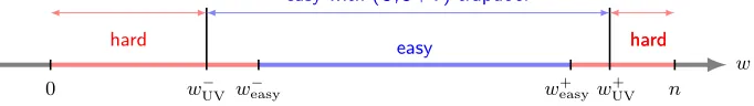
easy, ω+easy]⊆ [ω−, ω+] otherwise anybody that uses the generalized Prange algorithm would be able to invert fw,H. All of this is summarized in Figure 1 where we draw the above different areas asymptotically innofw/nwhenk/nis fixed andq= 3.
Fig. 1.Areas of relative signature distances whenq= 3.
Enlarging the Easy Domain Jw
− easy, w
+
easyK. Inverting the syndrome function fw,H is the
basic problem upon which all code-based cryptography relies. This problem has been studied for a long time for relative weights ω=4wn in (0, ω−easy) and despite many efforts the best algorithms [Ste88, Dum91, Bar97, MMT11, BJMM12, MO15, DT17, BM18] for solving this problem are all exponential in n for such fixed relative weights. In other words, after more than fifty years of research, none of those algorithms came up with a polynomial complexity for relative weights ω in (0, ωeasy− ). Furthermore, by adapting all the previous algorithms beyond this point we observe for them the same behaviour: they are all polynomial in the range of relative weights [ωeasy− , ωeasy+ ] and become exponential once again whenωis in (ω+
easy,1). All these results point towards the fact that invertingfw,H in polynomial time on a larger range is fundamentally a hard problem. In the following subsection we present a trapdoor on the matricesHthat enables to invert in polynomial timefw,H on a larger range by tweaking the Prange decoder.
3.3 Solution with Trapdoor
Jw −
UV, w +
UVK ⊂Jw −, w+
K but with Jw −
easy, weasy+ K (Jw −
UV, w +
UVK. We summarize this situation in
Figure 2.
We wish to point out here, to avoid any misunderstanding that the procedure we give here is not the one we use at the end to instantiate Wave, but is merely here to give the underlying idea of the trapdoor. Rejection sampling will be needed as explained in the following section to avoid any information leakage on the trapdoor coming from the outputs of the algorithm given here.
hard easy hardhard
w
0 w weasy− w+easy n
−
UV w
+ UV
easy with (U,U+V) trapdoor
Fig. 2.Hardness of (U, U+V) Decoding
It turns out that in the case of a normalized generalized (U, U+V)-code, a simple tweak of the Prange decoder will be able to reach relative weightsw/noutside the “easy” region [ωeasy− , ωeasy+ ]. It exploits the fundamental leverage of the Prange decoder : it consists in choosing the error e
satisfying eH| =s as we want in k positions when the code that we decode is random and of dimensionk. When we want an error of low weight, we put zeroes on those positions, whereas if we want an error of large weight, we put non-zero values. This idea leads to even smaller or larger weights in the case of a normalized generalized (U, U+V)-code. To explain this point, recall that we want to solve the following decoding problem in this case.
Problem 2 (decoding problem for normalized generalized (U, U +V)-codes). Given a normalized generalized (U, U+V) code (ϕ,HU,HV) (see Proposition 1) of parity-check matrixH=H(ϕ,HU,HV)∈ F(nq −k)×n, and a syndrome s∈Fqn−k, finde∈Fqn of weight wsuch thateH|=s.
The following notation will be very useful to explain how we solve this problem.
Notation 1 For a vectore inFn
q, we denote by eU andeV the vectors in Fn/2q such that (eU,eV) =ϕ−1(e).
The decoding algorithm we will consider recoverseV and theneU. From eU andeV we recovere sincee=ϕ(eU,eV). The point of introducing such aneU and aneV is that
Proposition 3. Solving the decoding problem 2 is equivalent to find an e ∈ Fnq of weight w satisfying
eUH|U =s
U (7)
eVH|V =s
V (8)
wheres= (sU,sV)with sU ∈
Fn/2q −kU andsV ∈Fn/2q −kV.
Remark 3. We have put U and V as superscripts in sU and sV to avoid any confusion with the notation we have just introduced foreU andeV.
Proof. Let us observe that,
e=ϕ(eU,eV) = (aeU+beV,ceU+deV) = (eUA+eVB,eUC+eVD) withA=Diag(a),B=Diag(b),C=Diag(c),D=Diag(d). By using this,eH|=stranslates into,
eUAD|H|U+eVBD|H|U−eUCB|H|U−eVDB|H|U =sU
which amounts to eU(AD−BC)H|U =s
U and e
V(AD−BC)H|V =s
V, since A, B, C, D are diagonal matrices, they are therefore symmetric and commute with each other. We finish the proof by observing thatAD−BC=In/2, the identity matrix of sizen/2. ut Performing the two decoding (7) and (8) independently with the Prange algorithm gains nothing. However if we first solve (8) with the Prange algorithm, and then seek a solution of (7) which properly depends on eV we increase the range of weights accessible in polynomial time for e. It then turns out that the range [ωUV− , ω+UV] of relative weights w/n for which the (U, U +V )-decoder works in polynomial time is larger than [ωeasy− , ω+
easy]. This will provide an advantage to the trapdoor owner.
Tweaking the Prange Decoder for Reaching Large Weights. Whenq= 2, small and large weights play a symmetrical role. This is not the case anymore forq≥3. In what follows we will suppose thatq≥3.In order to find a solutioneof large weight to the decoding problemeH|=s, we use Proposition 3 and first find an arbitrary solutioneV toeVH|V =sV. The idea, now for performing the second decodingeUH|U =s
U, is to take advantage ofe
V to find a solutioneU that maximizes the weight of e =ϕ(eU,eV). On any information set of the U code, we can fix arbitrarily eU. Such a set is of sizekU and on those positionsiwe can always chooseeU(i) such that this induces simultaneously two positions in e that are non-zero. These are ei and ei+n/2. We just have to chooseeU(i) so that we have simultaneously
aieU(i) +bieV(i)6= 0 cieU(i) +dieV(i)6= 0.
This is always possible sinceq≥3 andaici6= 0 for alliwhich gives an expected weight ofe:
E(|e|) = 2
kU + q−1
q (n/2−kU)
=q−1 q n+
2kU
q (9)
The best choice for kU is to takekU =kup to the point where q−q1n+2kq =n, that is k=n/2 and for larger values ofkwe choose kU =n/2 andkV =k−kU.
Why Is the Trapdoor More Powerful for Large Weights than for Small Weights? This strategy can be clearly adapted for small weights. However, it is less powerful in this case. Indeed, to minimize the weight of the final error we would like to chooseeU(i) inkU positions such that
aieU(i) +bieV(i) = 0 cieU(i) +dieV(i) = 0
Here as aidi −bici = 1 and aici 6= 0 in the family of codes we consider, this is possible if and only if eV(i) = 0. Therefore, contrarily to the case where we want to reach errors of large weight, the area of positions where we can gain twice is constrained to be of size n/2− |eV|. The minimal weight foreV we can reach in polynomial time with the Prange decoder is given by
q−1
q (n/2−kV). In this way the set of positions where we can double the number of 0 will be of size n/2−q−q1(n/2−kV) =2qn +q−q1kV. It can be verified that this strategy would give the following expected weight for the final error we get:
E(|e|) =
(q−1 q n−2
q−1
q kU ifkU ≤ 2qn + q−1
q kV 2(q−1)2
(2q−1)q(n−k) else.
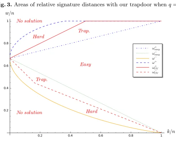
Fig. 3.Areas of relative signature distances with our trapdoor whenq= 3
4
Preimage Sampling with Trapdoor: Achieving a Uniformly
Distributed Output
We restrict here our study to the case,
q= 3.
All the results we are going to give can be generalized to larger values ofq. To be a trapdoor one-way preimage sampleable function, we have to enforce that the outputs of our algorithm, which inverts our trapdoor function, are very close to be uniformly distributed overSw. The procedure described in the previous section using directly the Prange decoder, does not meet this property. As we will prove, by changing it slightly, we will achieve this task by still keeping the property to output errors of weight w for which it is hard to solve the decoding problem for this weight. However, the parameters will have to be chosen carefully and the area of weights w for which we can output errors in polynomial time decreases. Figure 4 gives a rough picture of what will happen.
hard easy hardhard
w
0
weasy− w+easy
n
wUV− w
+ UV
easy with (U,U+V) trapdoor
no leakage with(U, U+V)trapdoor
Fig. 4.Hardness of (U, U+V) Decoding with no leakage of signature
4.1 Rejection Sampling to reach Uniformly Distributed Output
is uniformly distributed over the words of weightw when the syndrome sis randomly chosen in Fn3−k. Solving the decoding problem 2 of the generalized (U, U+V)-code will be done by solving (7) and (8) through an algorithm whose skeleton is given in Algorithm 2. DecodeV(HV,sV) returns a vector satisfyingeVH|V =sV, whereasDecodeU(HU, ϕ,sU,eV) is assumed to return a vector satisfyingeUH|U =s
U andsuch that|ϕ(e
U,eV)|=w. Heres= (sU,sV) withsU ∈Fn/23 −kU andsV ∈Fn/23 −kV.
Algorithm 2DecodeUV(HV,HU, ϕ,s)
1: repeat
2: eV ←DecodeV(HV,sV)
3: untilCondition 1 is met 4: repeat
5: eU←DecodeU(HU, ϕ,sU,eV) .We assume that|ϕ(eU,eV)|=where.
6: e←ϕ(eU,eV)
7: untilCondition 2 is met 8: return e
What we want to achieve by rejection sampling is that the distribution of e output by this algorithm is the same as the distribution of eunif that denotes a vector that is chosen uniformly at random among the words of weightwin Fn3. This will be achieved by ensuring that
1. theeV fed intoDecodeU(·) at Step 5 has the same distribution aseunifV ,
2. the distribution ofeU surviving to Condition 2 at Step 7 conditioned on the value ofeV is the same as the distribution ofeunifU conditioned on eunifV .
There is a property of the decoders DecodeV(·) andDecodeU(·) derived from Prange de-coders that we will consider that will be very helpful here. They will namely be very close to meet the following conditions.
Definition 3. DecodeV(·)is said to be weightwise uniform if the outputeV ofDecodeV(HV,sV) is such that P(eV) is just a function of |x| when sV is chosen uniformly at random in Fn/23 −kV.
DecodeU(·) is m1-uniform if the outputput eU of DecodeU(HU, ϕ,sU,eV) satisfies that the conditional probability P(eU|eV)is just a function of the pair(|eV|, m1(ϕ(eU,eV))where
m1(x)=4
1≤i≤n/2 :|(xi, xi+n/2)|= 1 .
It is readily observed that for allx∈Sw,
P(eunifV =xV) and P(eunifU =xU |eunifV =xV)
are also only functions of |xV| and (|xV|, m1(x)) respectively. From this it is readily seen that we obtain the right distributions for eV and eU conditioned on eV by just ensuring that the distribution of |eV| follows the same distribution as |eunifV | and that the distribution of m1(e) conditioned on |eV| is the same as the distribution of m1(eunif) conditioned on |eunifV |. This is shown by the following lemma.
Lemma 1. Letebe the output of Algorithm 2 whensV andsU are chosen uniformly at random in Fn/23 −kV andF
n/2−kU
3 respectively. Assume thatDecodeU(·)ism1-uniform whereasDecodeV(·) is weightwise uniform. If for any possibley andz,
|eV| ∼ |eunifV | and P(m1(e) =z| |eV|=y) =P(m1(eunif) =z| |eunifV |=y) (10) then
e∼eunif.
The probabilities are taken here over the choice of sU and sV and over the internal coins of
Proof. We have for anyxin Sw
P(e=x) =P(eU =xU |eV =xV)P(eV =xV)
=P(DecodeU(HU, ϕ,sU,eV) =xU |eV =xV)P(DecodeV(HV,sV) =xV) =P(m1(e) =z| |eV|=y)
n(y, z)
P(|eV|=y) n(y)
4
=P (11)
where n(y) is the number of vectors ofFn3 of weight y and n(y, z) is the number of vectors ein Fn3 such thateV =xV and such that m1(e) = z (this last number only depends onxV through its weight y). Equation (11) is here a consequence of the weightwise uniformity ofDecodeV(·) on one hand and them1-uniformity ofDecodeU(·) on the other hand. We conclude by noticing that
P =P(m1(e
unif) =z| |eunif V |=y) n(y, z)
P(|eunifV |=y)
n(y) (12)
=P(eunifU =xU |eunifV =xV)P(eunifV =xV)
=P(eunif =x). (13)
Equation (12) follows from the assumptions on the distribution of |eV| and of the conditional
distribution ofm1(e) for a given weight|eV|. ut
This shows that in order to obtain that e is uniformly distributed over Sw it is enough to perform rejection sampling based on the weight |eV| for DecodeV(·) and based on the pair (|eV|, m1(e)) forDecodeU(·). In other words, our decoding algorithm with rejection sampling will use a rejection vectorrV on the weights ofeV forDecodeV(·) and a two-dimensional rejection vectorrU for the values of (|eV|, m1(e)) forDecodeU(·). The corresponding algorithm is specified
in Algorithm 3.
Algorithm 3DecodeUV(HV,HU, ϕ,s)
1: repeat
2: eV ←DecodeV(HV,sV)
3: untilrand([0,1])≤rV(|eV|)
4: repeat
5: eU←DecodeU(HU, ϕ,sU,eV)
6: e←ϕ(eU,eV)
7: untilrand([0,1])≤rU(|eV|, m1(e))
8: return e
Standard results on rejection sampling yield the following proposition:
Proposition 4. Let,
q1(i)4=P(|eV|=i) ; q1unif(i)
4
=P |eunifV |=i
(14) q2(s, t)=4P(m1(e) =s| |eV|=t) ; qunif2 (s, t)
4
=P m1(eunif) =s| |eunifV |=t
(15) for any i, t∈J0, n/2Kands∈J0, tK. Let rV andrU be defined as
rV(i)=4 1 Mrs
V
qunif1 (i)
q1(i) and rU(s, t)
4
= 1
Mrs U(t)
q2unif(s, t) q2(s, t)
with
MVrs4= max 0≤i≤n/2
q1unif(i)
q1(i) and M rs U(t)
4
= max 0≤s≤t
q2unif(s, t) q2(s, t)
Then if DecodeV(·) is weightwise uniform and DecodeU(·) is m1-uniform, the output e of Algorithm 3 satisfies
4.2 Application to the Prange Decoder
To instantiate rejection sampling, we have to provide here (i) howDecodeV(·) andDecodeU(·) are instantiated and (ii) how qunif
1 , q2unif, q1 and q2 are computed. Let us begin by the following proposition (the proof is given in Appendix A) which givesqunif
1 andq2unif.
Proposition 5. Let nbe an even integer,w≤n,i, t≤n/2 ands≤t be integers. We have,
qunif1 (i) = n/2 i n w 2w/2 i X p=0 w+p≡0 mod 2
i
p
n/2
−i (w+p)/2−i
23p/2 (16)
q2unif(s, t) =
(t s)(
n/2−t w+s
2 −t) 232s
P p(
t p)(
n/2−t w+p
2 −t) 232p
ifw+s≡0 mod 2.
0 else
(17)
Algorithms DecodeV(·),DecodeU(·) are described in Algorithms 4 and 5. They use the rejection vectors given in Proposition 4 which is based on the expressions given in Proposition 5.
Algorithm 4DecodeV(HV,sV) the Decoder outputting aneV such thateVH|V =sV.
1: J,I ←FreeSet(HV)
2: `←-DV
3: xV ← -n
x∈Fn/3 2| |xJ|=`,Supp(x)⊆ I o
.(xV)I\J is random
4: eV ←PrangeStep(HV,sV,I,xV)
5: return eV
functionFreeSet(H) Require: H∈F(3n−k)×n
Ensure: Ian information set ofhHi⊥
andJ ⊂ I of sizek−d
1: repeat
2: J ←-J1, nKof sizek−d
3: untilthe rank of the columns ofHindexed byJ1, nK\J isn−k
4: repeat 5: J0←
-J1, nK\J of sized
6: I ← J t J0
7: untilI is an information set ofhHi⊥
8: returnJ,I
These two algorithms both use the Prange decoder in the same way as we did with the procedure described in§3.3 to reach large weights, except that here we introduced some internal distributions
DV and theDUt’s. These distributions are here to tweak the weight distributions of DecodeV(·) andDecodeU(·) in order to reduce the rejection rate. We have:
Proposition 6. Let n be an even integer, w≤n,i, t, kU ≤n/2 ands ≤t be integers. Let d be an integer, kV0 =4kV −d and kU0 =4kU −d. Let XV (resp. XUt) be a random variable distributed according to DV (resp.DtU). We have,
q1(i) = i
X
t=0
n/2−k0V i−t
2i−t 3n/2−k0
V P
(XV =t) (18)
q2(s, t) =
P
t+k0U−n/2≤k6=0≤t k0
4
=k0U−k6=0
(t−k6=0
s )(
n/2−t−k0 w+s
2 −t−k0) 232s
P p(
t−k6=0
p )(
n/2−t−k0
w+p
2 −t−k0) 232pP
(Xt
U =k6=0) if w≡smod 2.
0 else
Algorithm 5DecodeU(HU, ϕ,sU,eV) the U-Decoder outputting aneU such thateUH|U =s U and|ϕ(eU,eV)|=w.
1: t← |eV|
2: k6=0←-DtU
3: k0←k0U−k6=0 . kU0
4
=kU−d
4: repeat
5: J,I ←FreeSetW(HU,eV, k6=0)
6: xU←-{x∈F3n/2| ∀j∈ J, x(j)∈ {−/
bi
aieV(i),−
di
cieV(i)}and Supp(x)⊆ I} 7: eU←PrangeStep(HU,sU,I,xU)
8: until|ϕ(eU,eV)|=w
9: return eU
functionFreeSetW(H,x, k6=0)
Require: H∈F(qn−k)×n,x∈Fnq andk6=0∈J0, kK. Ensure: J andIan information set ofhHi⊥
such that|{i∈ J :xi6= 0}|=k6=0andJ ⊂ Iof sizek−d. 1: repeat
2: J1←-Supp(x) of sizek6=0
3: J2←-J1, nK\Supp(x) of sizek−d−k6=0.
4: J ← J1t J2
5: untilthe rank of the columns ofHindexed byJ1, nK\J isn−k
6: repeat 7: J0←
-J1, nK\J of sized
8: I ← J t J0
9: untilI is an information set ofhHi⊥
10: returnJ,I
A parameter dis introduced in Proposition 6 and in Algorithms 4 and 5. When 3d ≈2λ the probability for not being able to complete a set of k−dpositions into an information set of an [n, k] code is of order 21λ. In Algorithm 4 (resp. 5) we pick a set ofkV −d(resp.kU−d) random
positions. Those positions will be filled with the ad-hoc rule usingDV (resp.DtU). With probability at least 1− 1
2λ those sets can be completed with dextra positions to reach an information set.
Thosedpositions are filled randomly. We perform the Prange decoder and also fill the remaining n/2−kV (resp.n/2−kU) positions with random values. Doing things this way will allow us to prove that we are close enough to the two uniformity conditions of Definition 3. We are going to prove that,
Theorem 1. Letebe the output of Algorithm 3 based on Algorithms 4,5 andeunif be a uniformly distributed error of weightw. We have
P
ρ(e,eunif)>3−d/2≤3−d/2. where the probability is taken over the choice of matrices HU andHV.
A much stronger result showing that ρ(e,eunif) is typically smaller than n23−d will be given in the appendix. This result will be used to select the parameterdinstead of the previous theorem.
It will be helpful to consider now the following definition.
Definition 4 (Bad and Good Subsets). Let d ≤ k ≤ n be integers and H ∈ F(n3 −k)×n. A subsetE ⊆J1, nK of sizek−dis defined as a good set forHif HE is of full rank where E denotes the complementary of E. Otherwise, E is defined as a bad set for H.
The proof of this theorem relies on introducing a variant of the decoder based on variants of the U and V decoders VarDecodeV(·) and VarDecodeU(·) of algorithms DecodeV(·) and
DecodeU(·) respectively. These new decoders will work asDecodeV(·) andDecodeU(·) when
the exception that there is no guarantee that the error eV that is output by VarDecodeV(·) satisfieseVH|V =s
V or that thee
U that is output byVarDecodeU(·) satisfieseUH|U =s U. The
eV and eU that are output are chosen on the positions of J asDecodeV() andDecodeU() as would have done it, but the rest of the positions are chosen uniformly at random inF3. It is clear that in this case
Fact 2 VarDecodeV(·)is weightwise uniform andVarDecodeU(·)ism1-uniform.
The point of consideringVarDecodeV(·) and VarDecodeU(·) is that they are very good ap-proximations of DecodeV(·) and DecodeU(·) that meet the uniformity conditions that ensure by using Lemma 1 that the output of Algorithm 3 usingVarDecodeV(·) andVarDecodeU(·) instead ofDecodeV(·) and DecodeU(·) produces an errore that is uniformly distributed over the words of weightw. The outputs ofVarDecodeV(·) andVarDecodeU(·) only differ from the output ofDecodeV(·) andDecodeU(·) when a bad setJ is encountered. These considerations can be used to prove the following proposition.
Proposition 7. Algorithm 3 based onVarDecodeV(·)andVarDecodeU(·)produces uniformly distributed errorseunif of weightw. Letebe the output of Algorithm 3 with the use ofDecodeV(·) and DecodeU(·). Let Junif be uniformly distributed over the subsets of
J1, n/2K of size kV −d
whereas JHV is uniformly distributed over the same subsets that are good for H
V. Let IxunifV,` be
uniformly distributed over the subsets of J1, n/2K of size kU −d such that their intersection with
xV is of size ` whereas IxHVU,` is the uniform distribution over the same subsets that are good for
HU. We have: ρ e;eunif
≤ρ JHV;Junif+X
xV,`
ρIHU
xV,`;I
unif xV,`
P(k6=0=`|eV =xV)P eunifV =xV
Proof. The first statement about the output of Algorithm 3 is a direct consequence of Fact 2 and Lemma 1. The proof of the rest of the proposition relies on the following proposition [GM02, Proposition 8.10]:
Proposition 8. Let X,Y be two random variables over a common set A. For any randomized function f with domainA using internal coins independent fromX andY, we have:
ρ(f(X);f(Y))≤ρ(X;Y). Let us define forxV ∈Fn/23 and xU ∈Fn/23 ,
p(xV)
4
=P(eV =xV) ; q(xV)
4
=P eunifV =xV
p(xU|xV)
4
=P(eU =xU |eV =xV) ; q(xU|xV)
4
=P eunifU =xU |eunifV =xV. We have,
ρ e;eunif=ρ eU,eV;eunifU ,e unif V
=1 2
X
xV,xU
|p(xV)p(xU|xV)−q(xV)q(xU|xV)|
=1 2
X
xV,xU
|(p(xV)−q(xV))p(xU|xV) + (p(xU|xV)−q(xU|xV))q(xV)|
≤1
2
X
xV,xU
|(p(xV)−q(xV))p(xU|xV)|+|(p(xU|xV)−q(xU|xV)q(xV)|
=1 2
X
xV
|(p(xV)−q(xV))|+ 1 2
X
xV,xU
where in the last line we used thatP
xU|p(xU|xV)|= 1 for any xV. Thanks to Proposition 8:
1 2
X
xV
|p(xV)−q(xV)| ≤ρ JHV;Junif (21)
as the internal distribution DV of DecodeV(·) is independent ofJHV and Junif. Let us
upper-bound the second term of the inequality. The distribution ofk6=0 is only function of the weight of the vector given as input toDecodeU(·) orVarDecodeU(·). Therefore,
P(k6=0=`|eV =xV) =P k6=0=`|eunifV =xV
(22) Let us define,
p(xU|xV, `)
4
=P(eU =xU |k6=0=`,eV =xV) ; q(xU|xV, `)
4
=P(eunifU =xU |k6=0=`,eunifV =xV). With this notation we obtain from (22)
p(xU|xV)−q(xU|xV) =
X
`
(p(xU|xV, `)−q(xU|xV, `))P(k6=0=`|eV =xV) (23)
The internal coins ofDecodeU(·) and VarDecodeU(·) are independent of IHU
xV,` andI
unif xV,`and
by using Proposition 8 we have for anyxV and`: 1
2
X
xU
|p(xU|xV, `)−q(xU|xV, `)| ≤ρ
IHU
xV,`;I
unif xV,`
(24)
Combining Equations (20), (21), (23) and (24) concludes the proof. ut
The expectations ofρ JHV;Junifandρ
IHU
xV,`;I
unif xV,`
are upperbounded by
Lemma 2. We have
ρ JHV;Junif=#{subsets ofJ1, n/2K of sizek−dbad forH}
n/2 k−d
(25)
ρIHU
xV,`;I
unif xV,`
= |x| Nx,` `
n/2−|x|
k−d−`
(26)
Eρ JHV;Junif ≤3
−d
2 (27)
E
n
ρIHU
xV,`;I
unif xV,`
o ≤3
−d
2 , , (28)
where Nx,` is the number of subsets of J1, n/2K of size k−d such that their intersection with
Supp(x)is of size `and that are bad for H.
Proof. (25) (26) follow from the fact that that the statistical distance between the uniform dis-tribution overJ1, sK and the uniform distribution overJ1, tK (witht≥s) is equal to t−ts. Let us index from 1 to kn/2−d
the subsets of sizek−dofJ1, n/2Kand letXibe the indicator of the event “the subset of indexiis bad”. We have
N = (n/2
k−d)
X
i=1
Xi. (29)
Recall now (for a proof see Lemma 8 in the appendix) that for integersd < m:
when M is chosen uniformly at random in F(m3 −d)×m. This implies P(Xi = 1) ≤ 1 2·3d and
Eρ JHV;Junif =
E
N (n/2
k−d)
= P(
n/2
k−d)
i=1 P (Xi=1)
(n/2
k−d)
≤ 1
2·3d. This proves (27). (28) follows from
similar arguments.ut
We are ready now to prove Theorem 1.
Proof (of Theorem 1). By using Markov’s inequality we have P
ρ(e,eunif)>3−d/2≤3d/2E(ρ(e,eunif))
≤3d/2E
ρ JHV;Junif
+X
xV,`
ρIHU
xV,`;I
unif xV,`
P(k6=0=`|eV =xV)P eunifV =xV
(by Prop. 7)
≤3d/2
3−d 2 +
X
xV,`
3−d
2 P(k6=0=`|eV =xV)P e unif V =xV
(by Lem. 2)
= 3−d/2.
u t
4.3 Instantiating the Distributions
Any choice for the distributionsDV andDtU in Algorithms 4 and 5 will enable uniform sampling by a proper choice of the rejection vectorsrV andrU in Algorithm 3. We argue here, through a case study, that an appropriate choice of the distributions may considerably reduce the rejection rate. In fact, what matters is to have the smallest possible values forMrs
V andMUrs(t) in Proposition 4. The first step to achieve this is to correctly align the distributions to their targets, we do that by a proper choice for the mean value or of the mode (i.e. maximum value) of the distributions. Next we choose a “shape” for the distributions. Here we will take (generalized and truncated) Laplace distributions with a prescribed mean and parameterize them to minimize rejection.
For typical parameters with 128 bits of classical security, we will give a case study with the above strategy, in which the total rejection rate is below 1%.
Aligning the Distributions:
1. For the distributionDV. The output of Algorithm 4 has an average weight ¯`+2/3(n/2−kV+d), where ¯` denotes the mean of DV. It must be close to E(|eunifV |). We will admit E(|e
unif V |) =
Pn/2
i=0iq unif V (i) =
n 2
1− 1−w n
2 −1
2 w n
2
. The mean value ¯` of DV is chosen (close to) (1−α)(kV −d) whereα∈[0,1] is defined as follows
(1−α)(kV −d) =n 2
1−1−w
n
2 −1
2
w
n
2 −2
3
n
2 −kV +d
. (30)
2. For the distribution Dt
U, 0 ≤ t ≤ n/2. Here, for every t, we want to align the functions s7→q2(s, t) ands7→q2unif(s, t) (see Proposition 4). We get a very good estimate of theswhich maximizesqunif
2 (s, t) by solving numerically the equationq2unif(s−1, t) =q2unif(s+ 1, t), that is 8 (t−s) (t−s+ 1) (n−w−s+ 1)
(s+ 1)s(w+s+ 1−2t) = 1 We will denote mmax
s=mmax
target(t). For a givent,q2(s, t) is the probability to havem1(e) =s. This number counts the pairs (i, i+n/2) withi∈J0, n/2Ksuch that exactly one ofe(i) ande(i+n/2) is non-zero.
This may only happen when i ∈ Supp(eV)\ J, in which case e(i) and e(i+n/2) are two random distinct elements ofF3and this particulariis counted inm1(e) with probability 2/3. Since|Supp(eV)\ J |=t−k6=0, we typically havem1(e) = 23(t−k6=0) and the best alignment is reached when the most probable output of distributionDt
U isk6=0=t−32mmaxtarget(t).
Matching the “Shapes”: to avoid a high rejection rate we need to choose distributions so that the tails of the emulated q1 and q2 are not lower than their respective targets. A bad choice in this respect could lead to values ofMVrs andMUrs(t) growing exponentially with the block size. We chose generalized and truncated Laplace distributions to avoid this.
Definition 5 (Generalized Truncated Discrete Laplace Distribution).Let µ, σ, β be pos-itive real numbers, let a and b be two integers. We say that a random variable X is distributed according to the Generalized Truncated Discrete Laplace Distribution of parameters µ, σ, β, a, b, which is denoted X∼Lapβ(µ, σ, a, b), if for all i∈Ja, bK,
P(X=i) = e
−(|i−µ| σ )
β
N
whereN is a normalization factor.
We choose
DV = LapβV(µV, σV,0, kV −d)
Dt
U = LapβU(t)(µU(t), σU(t), t+kU−d−n/2, t)
with
µV = (1−α)(kV −d) µU(t) =t−32mmaxtarget(t) +ε(t) whereβV andσV are selected to minimizeMrs
V, andβU(t),ε(t), andσU(t) are selected to minimize MUrs(t). We observed heuristically that the exponents βV andβU(t) are in the interval [1,2], and that the alignment offsetε(t) is in the interval [0,2].
Case Study: n = 8482, (kU, kV) = (3558,2047), w = 7980, α = 0.5748 and d = 81. With σV = 30.31 andβV = 1.982, we obtainMVrs ≈1.000895. Withε= 0.29 and βU = 1.788 identical for all t, the optimal σU(t) lies in the interval [7.27,11.58], and we obtain an average value of 1.0086 forMrs
U(t). The result is marginally better by selecting the bestβU(t) andε(t) for eacht. The total rejection rate is thus below 1%.
4.4 Choosing the parameters
Using the parameterαintroduced in (30) in the previous subsection as
(1−α)(kV −d) =n 2
1−1−w
n
2 −1
2
w
n
2 −2
3
n
2 −kV +d
.
we may define all the system parameters depending only onα, the code ratek/n,dand the block sizen
w=
$
n 1−α+1 3
s
(3α−1)
3α+ 4k−2d n −1
!%
(31)
kV =d+
n
2 3 3α−1
1−w
n
2
+1 2
w
n
2 −1
3
;kU =d+jn 2
−2 + 3w n
k
5
Achieving Uniform Domain Sampling
The following definition will be useful to understand the structure of normalized generalized (U, U+ V)-codes.
Definition 6. (number of V blocks of type I).In a normalized generalized (U, U +V)-code of length nassociated to (a,b,c,d), the number of V blocks of type I, which we denote by nI, is defined by:
nI=4|{1≤i≤n/2 :bidi= 0}|.
Remark 4. nI can be viewed as the number of positions in which a codeword of the form (b
v,dv) is necessarily equal to 0: this comes from the fact that on a position where eitherbi= 0 or di = 0, the other one is necessarily different from 0 as aidi−bici = 1. In other words we also have
nI =|{1≤i≤n/2 :bi= 0}|+|{1≤i≤n/2 :di = 0}|.
We denote byHpkthe public parity-check matrix of a normalized generalized (U, U+V)-code as described in §2.2. It turns out that Hpk has enough randomness in it for making the syndromes associated to it indistinguishable in the strongest possible sense, i.e. statistically, from random syndromes as the following proposition shows. In other words, our scheme achieves the Domain Sampling property of Definition 1. Note that the upper-bound we give here depends on the number nI we have just introduced.
Proposition 9. LetDH
w be the distribution ofeH|wheneis drawn uniformly at random among Sw and letU be the uniform distribution over Fn3−k. We have
EHpk
ρ(DHpk w ,U)
≤ 1
2
√
ε with,
ε= 3 n−k 2w n w
+ 3
n/2−kV
n/2
X
j=0 qunif
1 (j)2 2j n/2
j
+ 3
n/2−kU
nI
X
j=0 nI
j
n−nI
w−j
2
n w
2
2j wherequnif
1 is given in Proposition 5 in§4.
This bound decays exponentially in nin a certain regime of parameters as shown by
Proposition 10. Let RU
4
=2kU
n ,RV
4
=2kV
n ,R
4
=k n,ω
4
=w n,ν
4
=nI
n, then under the same assump-tions as in Proposition 9, we have asntends to infinity
EHpk
ρ(DHpkw ,U)
≤2(α+o(1))n
whereα=412min ((1−R) log2(3)−ω−h2(ω), α1, α2)and
α1=4 min (x,y)∈R
1
2(1−RV) log23−ω−2h2(ω) + h2(x)
2 +x
h2(y) +3 2y−
1 2
+ (1−x)h2
ω−x(1−y)
1−x
R=4{(x, y)∈[0,1)×[0,1] : 0≤ω−x(1−y)≤1−x}
α2
4
= min
max(0,ω+ν−1)≤x≤min(ν,ω) 1
2(1−RU) log23−2h2(ω) +νh2
x
ν
+ 2(1−ν)h2
ω−x
1−ν
−x.
Remark 5. For the set of parameters we present in the appendix, we have ε ≈ 2−354 and α ≈
−0.02135. Note that the upper-bound of Proposition 9 is by no means sharp, this comes from the 3n2−kU
PnI
j=0 (nI
j)( n−nI
w−j)
2 (n w) 2 2j
The proof of this proposition relies among other things on the following variation of the left-over hash lemma (see [BDK+11]) that is adapted to our case: here the hash function to which we apply the left-over hash lemma is defined as h(e) =eH|pk. Functions hdo not form a universal family of hash functions (essentially because the distribution of theHpk’s is not the uniform distribution overF(n3 −k)×n). However in our case we can still bound εby a direct computation.
Lemma 3. Consider a finite family H= (hi)i∈I of functions from a finite set E to a finite set F. Denote byε the bias of the collision probability, i.e. the quantity such that
Ph,e,e0(h(e) =h(e0)) =
1
|F|(1 +ε)
where his drawn uniformly at random in H, eand e0 are drawn uniformly at random in E. Let
U be the uniform distribution over F and D(h) be the distribution of the outputsh(e)when e is chosen uniformly at random in E. We have
Eh(ρ(D(h),U))≤ 1 2
√
ε.
This lemma is proved in Appendix §C.1. In order to use this lemma to bound the statistical distance we are interested in, we used the following lemma.
Lemma 4. Assume thatx andy are random vectors ofSw that are drawn uniformly at random in this set. We have
PHpk,x,y xH|pk=yH
|
pk
≤ 1
3n−k(1 +ε)withε given in Proposition 9. Proof. By Proposition 3, the probability we are looking for is:
P (xU −yU)H|U =0and (xV −yV)H|V =0
where the probability is taken overHU,HV,x,y. To compute this probability we will use a stan-dard result, namely the following lemma.
Lemma 5. Letybe a non-zero vector ofFn3 andsan arbitrary element inFr3. We choose a matrix
H of sizer×nuniformly at random among the set ofr×nternary matrices. In this case
P yH|=s= 1 3r
Proof. The coefficient ofHat rowiand columnj is denoted byhij, whereas the coefficients ofy
andsare denoted by yi andsi respectively. The probability we are looking for is the probability to have
X
j
hijyj =si (33)
for all i in J1, rK. Since y is non zero, it has at least one non-zero coordinate. Without loss of generality, we may assume that y1 = 1. We may rewrite (33) as hi1 = P
j>1hijyj. This event happens with probability 13 for a given i and with probability 31r on all r events simultaneously
due to the independence of thehij’s. ut
This leads us to distinguish between the events:
Event 1:E1
4
={xU =yU and xV 6=yV} ; Event 2:E2
4
={xU 6=yU and xV =yV}
Event 3:E3
4
={xU 6=yU and xV 6=yV} ; Event 4:E4
4