Efficient Post-Quantum Zero-Knowledge and Signatures
(Draft)
Steven Goldfeder Princeton
Melissa Chase Microsoft Research
Greg Zaverucha Microsoft Research
November 22, 2017
Abstract
In this paper, we present a new post-quantum digital signature algorithm that derives its security entirely from assumptions about symmetric-key primitives, which are very well studied and believed to be quantum-secure (with increased parameter sizes). We present our new scheme with a complete post-quantum security analysis, and benchmark results from a prototype implementation.
Our construction is an efficient instantiation of the following design: the public key isy=f(x) for preimage-resistant functionf, andxis the private key. A signature is a non-interactive zero-knowledge proof ofx, that incorporates a message to be signed. Our security analysis uses recent results of Unruh (EUROCRYPT’12,’15,’16) that show how to securely convert an interactive sigma protocol to a non-interactive one in the quantum random oracle model (QROM). The Unruh construction is generic, and does not immediately yield compact proofs. However, when we specialize the construction
to our application, we can reduce the size overhead of the QROM-secure construc-tion to 1.6x, when compared to the Fiat-Shamir transform, which does not have a rigorous post-quantum security analysis. Our implementation results compare both instantiations, with multiple choices off for comparison. Our signature scheme pro-posal uses the block cipher LowMC forf, as it gives the shortest signatures.
In addition to reducing the size of signatures with Unruh’s construction, we also improve the size of proofs in the underlying sigma protocol (of Giacomelli et al., USENIX’16) by a factor of two. This is of independent interest as it yields more compact proofs for arbitrary choices of f in the classical case as well. Further, this reduction in size comes at no additional computational cost.
1
Introduction
with a generic transform similar to the well-known Fiat-Shamir (FS) transform [9]. As the basis of our scheme, we use the recently proposed ZKB proof system [10], which allows for proving statements of the form, “I knowxsuch thatf(x) =y”, wheref can be an arbitrary function such as SHA-256. Our key generation algorithm will make use of a functionf that is assumed to be preimage resistant against a quantum adversary. That is, for a uniformly distributedx, giveny=f(x), it is difficult to find anx0such thatf(x0) =y. The signature will then be a non-interactive a proof-of-knowledge ofx, that incorporates the message to be signed (as in the FS transform). This way of designing a signature scheme is similar to one described by Bellare and Goldwasser [2], but differs in the way the message is bound to the proof. In our scheme the message may be hashed when computing the challenge in the proof.
Using a NIZK proof of a preimage for an arbitrary functionf is appealing, since public and private keys are short, key generation is simple, and the security off is well understood (or commonly assumed). The two main challenges to make this practical are (1) efficiently realizing the NIZK proof and (2) post-quantum security analysis NIZK.
ZKB builds on the MPC-in-the-head paradigm of Ishai et al. [12], that we describe informally here. The multiparty computation protocol (MPC) will implement f, and the input is the witness x. For example, the MPC could compute y = SHA-256(x) where parties each have a share of x and y is public. The idea is to have the prover simulate a multiparty computation protocol “in his head”, commit to the state and transcripts of all players, then have the verifier “corrupt” a random subset of the simulated players by seeing their complete state. The verifier then checks that the computation was done correctly from the perspective of the corrupted players, and if so, he has some assurance that the output is correct. Iterating this for many rounds then gives the verifier high assurance.
In terms of practicality, each round is very computationally efficient, as it requires no number theoretic computations. The results of [10] have shown that computational costs are practical, even with an unoptimized implementation. The main challenge is signature size. Each round of the ZKB protocol outputs a transcript of the MPC protocol, and a large number of rounds are required for soundness. For example, for 80-bits of security against a classical attacker, ZKB proof of a SHA-256 preimage requires 137 rounds and is 835KB.
We made many improvements to ZKB, that taken together reduces the proof size by a factor of two when compared to [10]. We reduce the amount of randomness needed for each round of the protocol. In the original protocol, there were three independent sources of randomness: (1) the randomness to compute a secret sharing of the witness for the relation being proved, (2) a random seed for a PRG, and (3) randomness for the commitments. we show how it is sufficient (without making any additional hardness assumptions) to use a single source of randomness; the seed for the PRG.
cost. The comparison happens indirectly, when the hash of the recomputed transcripts are compared to the hash provided in the proof.
Moving to quantum safe parameters requires more that 137 rounds however, 438 by our analysis, so it is clear that proofs of SHA-256 preimages are too large. There is much flexi-bility in the choice off, and we chose a block cipher optimized for MPC called LowMC [1]. LowMC is designed to minimize the number of non-linear operations (multiplication gates),
to reduce the amount of communication required by MPC protocols. Choosing f as an
instance of LowMC reduces signature sizes dramatically. Our most efficient quantum safe parameter set at the 128-bit security level has 150KB signatures.
The second main challenge is the security analysis of the NIZK. It is not difficult to show that the interactive ZKB protocol is secure against a quantum adversary (with suitable parameters to account for generic advantage based on Grover’s algorithm). The difficulty is when transforming ZKB to a non-interactive proof. The Fiat-Shamir transform is simple and efficient, however, it lacks a proof in the quantum random oracle model (QROM). There are no known quantum attacks on the transform either, and many papers assume post-quantum security of FS signatures, if the primitives of the sigma protocol are quantum safe. See [4, 7] for more details.
In a series of papers [14, 15, 16], Unruh studies this problem, and presents a generic transform for turning a sigma protocol into a signature scheme with a security proof in the QROM. However, the ZKB protocol doesn’t completely match the properties that Unruh’s analysis requires. We show how to modify Unruh’s security proof to apply to ZKB.
We also give concrete parameters and an implementation for both the Unruh and FS transforms and ZKB, and measure the overhead of Unruh’s transform over regular Fiat-Shamir. The Unruh construction is generic, and does not immediately yield compact proofs. However, when we specialize the construction to our application, we find the overhead was surprisingly low, as a generic application of Unruh’s transform incurs a 4x increase in cost when compared to FS. For our LowMC parameter set targeting 128-bits of post-quantum security, the signature size overhead is about 1.6x (150KB for Unruh vs. 91KB for FS). In our current implementation the CPU overhead is roughly a factor of 1.2x. This shows that choosing a transform with a strong post-quantum security analysis can be practical.
2
Preliminaries and Definitions
Our definition of sigma protocols follows [6]. For a more formal definition, see [7].
Sigma protocol Asigma protocol(equivalently denoted Σ-protocol) is a three flow pro-tocol between a prover P and verifier V where transcripts have the form (r, c, s) where r
and sare computed byP and cis a challenge chosen by V. Let f be a relation such that
f(x) = y, where y is common input and x is a witness known only to P. V accepts if
(r, c, s) and (r, c0, s0) wherec6=c0, there is an efficient algorithm to extract a witnessx0 such thatf(x0) =y. There also exists an efficient simulator, given y and a randomly chosen c, outputs a transcript (r, c, s) fory that is indistinguishable from a real run of the protocol forx, y.
n-special soundness The sigma protocol described in the previous paragraph is 2-special sound, since two transcripts with different challenges are sufficient to extract a witness. A sigma protocol has n-special soundnessif n transcripts (r, c1, s1), . . .(r, cn, sn)
with distinctci guarantee that a witness may be efficiently extracted.
The following definition of a pseudorandom function (PRF) is specialized to this work; it uses a common parameter for the key, input and output length. The notationDFn means thatD is given oracle access toFn.
Definition 1 (Pseudorandom Function) Let F :{0,1}n× {0,1}n→ {0,1}n be an effi-ciently computable, length-preserving keyed function. We say thatF is a pseudorandom function (PRF), if for all probabilistic polynomial time distinguishers D,
|Pr[DFk(1n) = 1]−Pr[Dfn(1n) = 1]|
is negligible where k← {0,1}n is chosen uniformly at random and f
n is chosen uniformly at random from the set of functions mapping n-bit strings to n-bit strings.
We now define a weaker notion of a pseudorandom function in which we put an upper bound on the number of queries that the distinguisher can make to its oracle.
Definition 2 (q-Pseudorandom Function) Let Fk and fn be as defined in Definition 1, and letq be a positive integer constant. We say thatF is aq-pseudorandom function (q-PRF) if for all probabilistic polynomial time distinguishersDthat make at mostqqueries to their oracle,
|Pr[DFk(1n) = 1]−Pr[Dfn(1n) = 1]|
is negligible.
Clearly, a pseudorandom function is also aq-pseudorandom function for any constantq. When considering concrete security of PRFs against quantum attacks, we assume that an
n-bit function providesn/2 bits of security. In particular we make this assumption about the LowMC block cipher with the parameters chose in Section 5.
This paper requires a simple type of PRG a stateless function that expands a seed to a random string.
Concretely, we assume that AES-256 in counter mode provides 128 bits of PRG security, when used to expand 256-bit seeds to outputs less than 1KB in length.
Definition 4 (Preimage Resistance) Let H:{0,1}∗ → {0,1}nbe a cryptographic hash function. H is said to be preimage-resistant if, given y ∈ {0,1}n, finding an x ∈ {0,1}∗ such thatH(x) =yis is computationally intractable, i.e., costs at least O(2n/2) operations.
In the classical case it is common to assumeO(2n) operations for standard hash functions. When considering quantum algorithms, Grover’s algorithm can find preimages withO(2n/2) operations.
Definition 5 (Collision Resistance) Let H:{0,1}∗ → {0,1}n be a cryptographic hash function. H is said to be collision-resistant if finding a pair (x, x0) such that x 6= x0 is computationally intractable, i.e., costs at least 2n/2 operations.
When considering quantum algorithms, in theory it may be possible to find collisions using a generic algorithm of Brassard et al. [5] with costO(2n/3). A detailed analysis of the costs of the algorithm in [5] by Bernstein [3] found that in practice the quantum algorithm is unlikely to outperform theO(2n/2) classical algorithm. Multiple cryptosystems have since made the assumption that standard hash functions with n-bit digests provide n/2 bits of collision resistance against quantum attacks (for examples, see papers citing [3]). We make this assumption as well, and in particular, that SHA-256 provides 128 bits of PQ security. A computationally secure commitment scheme allows a sender to commit to a message such that given the transcript of the commitment phase the receiver, a computationally bound receiver cannot guess the committed message with probability non-negligibly better than at random. The sender is computationally bound to the committed message, i.e. cannot open to another message with greater than negligible probability.
Definition 6 (Commitment Scheme) Formally a (non-interactive) commitment scheme consists of three algorithms KG, Com, Verwith the following properties:
• KGis the key generation algorithm, on input the security parameter it outputs a public keypk.
• Comis the commitment algorithm. On input of a messageM it outputs[C(M), D(M)] =
Com(pk,M, R) where R are the coin tosses. C(M) is the commitment string, while D(M) is the decommitment string which is kept secret until opening time.
• Ver is the verification algorithm. On input C, D, it either outputs a message M or
⊥.
We note that if the sender refuses to open a commitment we can setD=⊥andVer(pk,C,⊥) =
Correctness If [C(M), D(M)] =Com(M, R) then Ver(pk, C(M), D(M)) =M.
Secure hiding For every message pair M, M0 the probability ensembles {C(M)}n∈N and
{C(M0)}n∈N are computationally indistinguishable for security parameter n.
Secure Binding We say that an adversaryAwins if it outputsC, D, D0 such thatVer(C, D) =
M, Ver(C, D0) = M0 and M 6=M0. We require that for all efficient algorithms A, the probability thatA wins is negligible in the security parameter.
To simplify our notation, we will often not explicitly write the public key pk when we make use of commitments. Our implementation uses hash-based commitments, which requires modeling the hash function as a random oracle in our security analysis. Note also that randomizing theComfunction may not be necessary if M has high entropy.
3
ZKB++
ZKB is a new proof system for zero-knowledge proofs on arbitrary circuits described in [10]. We describe the protocol here, but also present ZKB++, a much improved version of ZKB which enables proofs that are less than half the size of ZKB1.
3.1 ZKB
We now present the details of of the ZKB protocol. While ZKB is presented with various possible parameter options, we present only the final version with the best parameters. Moreover, while ZKB presents both interactive and non-interactive protocol versions, we present only the non-interactive version since our main goal is building a signature scheme for which we need the non-interactive version. In ZKB, the non-interactive version is not fully specified, so we refer to the accompanying implementation to fill in details where necessary.
Overview
ZKB builds on the MPC-in-the-head paradigm of Ishai et al. [12], that we describe only informally here. The multiparty computation protocol (MPC) will implement the relation, and the input is the witness. For example, the MPC could computey= SHA-256(x) where players each have a share of x and y is public. The idea is to have the prover simulate a multiparty computation protocol “in his head”, commit to the state and transcripts of all players, then have the verifier “corrupt” a random subset of the simulated players by seeing their complete state. The verifier then checks that the computation was done correctly from the perspective of the corrupted players, and if so, he has some assurance that the output is correct. Iterating this for many rounds then gives the verifier high assurance.
1
ZKB implements the idea of [12] as follows. In order to prove knowledge of a witness for a relationr :={(x, y), φ(x) =y}, we begin with a circuit that computesφ, and then the circuit is first decomposed into three parts. Intuitively, the decomposition is a three player MPC – it contains asharefunction that splits the input into three shares, three functions
outputi∈{1,2,3}that take as input all of the input shares and some randomness and produce an output share for each of the parties, and a function reconstructthat takes as input the three output shares and reconstructs the circuit’s final output. The decomposition is correct, and has 2-privacywhich intuitively means that revealing the views of any two players does not leak information about the witnessx.
With this decomposition, ZKB then uses the MPC-in-the-head technique to prove knowledge ofx. The prover simulatesnindependent runs of the three player MPC protocol and commits to the views – 3 views per run. The 3-party MPC protocol has a2-privacy
property, which informally means that if for each run, two players are corrupted and the adversary learns their view,xstill remains private. Then, using the Fiat-Shamir heuristic, the prover sends the commitments and output shares from each view to the random oracle computes a challenge – the challenge tells the prover which two of the three views to open for each of the n runs. Because of the two-privacy property, opening two views for each run does not leak information about the witness. The number of runs, n, is chosen to achieve negligible soundness error – i.e. intuitively it would be infeasible for the prover cheat without getting caught in at least one of the runs. The verifier checks that (1) the output of the each of the three views reconstructs toy, (2) each of the two open views were computed correctly, and (3) the challenge was computed correctly.
We now give a detailed description of the non-interactive ZKB protocol. Throughout this paper, when we do arithmetic on the indices of the players, there’s an implicit mod3 that omit to simplify the notation.
Definition 7 ((2,3)-decomposition) Let f(·) be a function that is computed by an n -gate circuit φ such that f(x) = φ(x) = y. Let k1, k2, and k3 be tapes of length κ chosen
uniformly at random from {0,1}κ corresponding to players P
1, P2 and P3, respectively.
Consider the following set of functions, D:
(view(0)1 ,view(0)2 ,view3(0))←Share(x, k1, k2, k3)
view(ij+1)←Update(viewi(j),view(i+1j), ki, ki+1) yi←Output(Viewi)
y←Reconstruct(y1, y2, y3)
The function Update computed the MPC for the next gate and updates the view accord-ingly. The function Outputi takes as input the final view, Viewi ≡view(in) after all gates have been computed and outputs player Pi’s output share, yi.
We define the following experiment EXP(decompφ,x) which runs the decomposition over a circuit φ on input x:
EXP(decompφ,x) :
1. First run theShare function onx: view(0)1 ,view(0)2 ,view(0)3 ←Share(x, k1, k2, k3)
2. For each of the three views, call the update function successively for every gate in the circuit: view(ij) =Update(viewi(j−1),view(ij+1−1), ki, ki+1) for i∈[1,3], j ∈[1, n]
3. From the final views, compute the output share of each view: yi←output(Viewi)
We say that D is a (2,3)-decomposition of φ if the following two properties hold when runningEXP(decompφ,x) :
(Correctness) For all circuits φ, for all inputsx and for theyi’s produced by , for all circuits φ, for all inputs x,
Pr[φ(x) =Reconstruct(y1, y2, y3)] = 1
(2-Privacy) Let D be correct. Then for all e∈ {1,2,3} there exists a PPT simulator
Se such that for any probabilistic polynomial-time (PPT) algorithm A, for all circuits φ, for all inputs x, and for the distribution of views and ki’s produced byEXP(decompφ,x) ,
Pr[A(x, y, ke,Viewe, ke+1,Viewe+1, ye+2) = 1]−Pr[A(x, y,Se(φ, y)) = 1]
is negligible.
3.1.1 The linear decomposition of a circuit
ZKB uses an explicit (2,3)-decomposition, which we recall here. Let R be an arbitrary finite ring and φ a function such that φ : Rm → R` can be expressed by an n-gate arithmetic circuit over the ring using addition by constant, multiplication by constant, binary addition and binary multiplication gates. A (2,3)−decomposition of φis given by the following functions. In the notation below, arithmetic operations are done inRswhere the operands are elements ofRs):
• (x1, x2, x3) ← share(x, k1, k2, k3) samples random x1, x2, x3 ∈ Rm such that x1 +
• view(ij+1) ←updatei(j)(viewi(j),view(i+1j) , ki, ki+1) computesPi’s view of the output wire
of gate gj and appends it to the view. Notice that it takes as input the views and
random tapes of both partyPi as well as party Pi+1. We usewk to refer to thek-th
wire, and we use wk(i) to refer to the value of wk in party Pi’s view. The update
operation depends on the type of gategj, and are defined as follows:
– case 1: addition by constant (wb =wa+k).
w(bi)=
(
wa(i)+k, ifi= 1
wa(i), otherwise
– case 2: multiplication by constant (wb=wa×k).
w(bi) =k×w(ai)
– case 3: binary addition (wc=wa+wb).
wc(i) =wa(i)+w(bi)
– case 4: binary multiplication (wc=wa×wb).
wc(i)=wa(i) ×w(bi) +
w(ai+1)×w(bi) +
w(ai) ×w(bi+1)+
Ri(c)−Ri+1(c)
whereRi(c) is thec-the output of a pseudorandom generator seeded with ki.
Note that with the exception of case 1, the gates are symmetric for all players. Also note that Pi can compute all gate types locally with the exception of binary
multiplication gates as this requires inputs from Pi+1. In other words, for every operation except binary multiplication, theupdatefunction does not use the inputs from the second party, i.e.,view(i+1j) and ki+1.
• yi ←outputi(view
(n)
i ) selects the ` output wires of the circuit as stored in the view view(in).
• y←reconstruct(y1, y2, y3) =y1+y2+y3
3.1.2 Choice of R
The functions that we work with in this paper are mostly specified on the bit-level, and therefore a natural choice for the ring is Z2. For a boolean circuit then, bitwise AND
operations (i.e. binary multiplication) require communication among parties, but XOR and INV gates can be computed locally.
3.1.3 ZKB Complete Protocol
Given a (2,3)-decomposition D for a function φ, the ZKB protocol is a zero knowledge proof system for relations of the form R := {(y, x) : y = φ(x)}. We recall the details of ZKB in Figure 3.1.3.
The ZKB non-interactive proof system
For public φ and y∈Lφ, the prover has x :y =φ(x). Com(·) is a secure commitment
scheme. The prover and verifier have access to a hash functionH(·).The integert is the number of parallel iterations.
p←Prove(x):
1. For each iteration ri, i∈[1, t]:
(a) Sample random tapesk(1i), k2(i), k3(i)
(b) Simulate the MPC protocol “in the head” to get an output viewView(ji)
and output shareyj(i)for each player . In particular, for each playerPj:
i. (x(1i), x2(i), x(3i)) =Share(x, k1(i), k2(i), k(3i))
ii. View(ji)=Update(Update(· · ·Update(x(ji), xj(i+1) , k(ji), k(ji+1) ). . .). . .). . .)
iii. y(ji) =Output(View(ji))
iv. Commit: [Cj(i), D(ji)] =Com(kj(i),View(ji))
(c) Denotea(i)= (y(i) 1 , y
(i) 2 , y
(i) 3 , C
(i) 1 , C
(i) 2 , C
(i) 3 )
2. Compute the challenge: e=H(a(1), a(2),· · · , a(t)). Interpret the challenge such that for i∈[1, t], e(i)∈ {1,2,3}
3. For each iteration ri, i∈[1, t], Denote z(i) = (D(ei), D(ei+1) )
4. Outputp= [(a(1), z(1)),(a(2), z(2)),· · · ,(a(t), z(t))]
1. Compute the challenge: e0 =H(a1, a2,· · · , at). Interpret the challenge such that
fori∈[1, t], e0(i)∈ {1,2,3}
2. For each iteration ri, i∈[1, t]:
(a) If∃j∈ {e0(i), e0(i)+ 1}s.t. Ver(Cj(i), Dj(i)) =⊥, outputReject
(b) Else,∀j∈ {e0(i), e0(i)+ 1},
{kj(i),View(ji)}=Ver(Cj(i), Dj(i))
(c) IfReconstruct(y1(i), y2(i), y(3i))6=y, output Reject
(d) If∃j∈ {e0(i), e0(i)+ 1}s.t. yj(i)6=Output(View(ji)), outputReject
(e) For each wire valuewj(e)∈Viewe, if
wj(e)6=update(viewe(j−1),viewe(j+1−1), ke, ke+1)
outputReject
3. output Accept
3.1.4 Serializing the views: ZKB approach
In the decomposition as described in Definition 7, the view is updated with the output wire value for each gate. While conceptually a player’s view includes the values that they computed locally, when the view is serialized, it is sufficient to include only the wire values of the gates that require non-local computations (i.e., the binary multiplication gates). The verifier can recompute the parts of the view due to local computations, and they don’t need to be serialized. Giving the verifier locally computed values does not even save any computation as the verifier will still need to recompute the values in order to check them.
In the ZKB paper, the serialized view included the following:
• input share
• output wire values for binary multiplication gates
• output share
The size of a view depends on the circuit as well as the ring that it is computed over. Let φ : (Z2`)m → (Z2`)n be the circuit being computed over Z2` such that there are m
|Viewi|=`(m+n+b)
3.1.5 ZKB proof size
Continuing with the above notation, we can now calculate the size of the ZKB proofs. Indeed the sizes that we give correspond to the sizes that were output by the ZKB reference code and reported in their paper. Recall from Figure 3.1.3 that for each iteration, a proof includes
1. a = (y1, y2, y3, C1, C2, C3), where yi is the output share of party Pi and ci is the
commitment toViewi
2. z= (De, De+1), where e∈ {1,2,3}is the challenge.
Assume that the random tapes are of size κ, and the commitments are of size c bits. In the hash based commitment scheme used by ZKB, the openingsDof the commitments contain the value being committed to as well as the randomness used for the commitments. Letsdenote the size of the randomness in bits used for each commitment. The size of the output share yi is the same as the output size of the circuit, (`×n). Assume that there
arer iterations.The total proof size is thus given by
|p|=r×[|a|+|z|]
=r×[3×(|yi|+|ci|) + 2×(|Viewi|+|ki|+s)]
=r×[3×(`n+c) + 2×(`×(m+n+b+s) +κ)] =r×[3c+ 2κ+ 2s+`×(5n+ 2m+ 2b)]
3.1.6 Commitment scheme used by ZKB
3.2 ZKB++
We now present ZKB++, a modification of ZKB. While the protocol follows along the same lines, we have several observations that allow us to reduce the proof size to less than half of the size in the original ZKB protocol. Moreover, our benchmarks show that this size reduction comes at no extra computational cost.
3.2.1 Modification 1: A modification of the decomposition
We therefore specify sampling as follows: (x1, x2, x3)←Share(x, k1, k2, k3) =:
x1 =R1(0)
x2 =R2(0)
x3 =x−x1−x2
As before, Ri is a pseudorandom generator seeded withki.
We note that sampling in this manner preserves the 2-privacy of the decomposition. In particular, given only two of {(k1, x1),(k2, x2),(k3, x3)}, x remains uniformly distributed over the choice of the third unopened (ki, xi).
We specify the Share function in this manner as it will lead to more compact zero-knowledge proofs. Moving now to the ZKB protocol, for each round, the prover is required to “open” two views. In order to verify the proof, the verifier must be given both the random tape and the input share for each opened view. If these values are generated independently of one another, then the prover will have to explicitly include both of them in the proof. However, with our sampling method, in View1 and View2, the prover only needs to includeki asxi can be deterministically computed by the verifier.
The exact savings depends on which views the prover must open, and thus depends on the challenge. The expected reduction in proof size resulting from using the ZKB++ sampling technique instead of the technique used in ZKB is
r× 4
3× |x|bits
Given a (2,3)-decomposition Dfor a functionφ, the ZKB++ protocol is a zero knowl-edge proof system for relations of the formR :={(y, x) :y=φ(x)}. We recall the details of ZKB++ in Figure 3.2.1.
The ZKB++ non-interactive proof system
For public φ and y ∈ Lφ, the prover has x : y = φ(x). The prover and verifier have
access to a Random Oracle H(·).t is the number of parallel iterations.
p←Prove(x):
1. For each iteration ri, i∈[1, t]:
(a) Sample random tapesk(1i), k2(i), k3(i)
(b) Simulate the MPC protocol “in the head” to get an output viewView(ji)
i.
(x(1i), x2(i), x(3i))←Share(x, k1(i), k2(i), k(3i))
= (G(k1(i)), G(k2(i)), x⊕G(k1(i))⊕G(k(2i)))
ii. View(ji)=Update(Update(· · ·Update(x(ji), xj(i+1) , k(ji), k(ji+1) ). . .). . .). . .)
iii. y(ji) =Output(View(ji))
iv. Commit: [Cj(i), Dj(i)] = [H(k(ji),Viewj(i)), kj(i)||View(ji)]
(c) Denotea(i)= (y1(i), y(2i), y3(i), C1(i), C2(i), C3(i))
2. Compute the challenge: e=H(a(1), a(2),· · · , a(t)). Interpret the challenge such that for i∈[1, t], e(i)∈ {1,2,3}
3. For each iteration ri, i∈[1, t],
(a) Denoteb(i)= (ye(i()i)+2, C
(i)
e(i)+2)
(b) Denotez(i)=
ife(i)= 1, (View2(i), k(1i), k2(i))
ife(i)= 2, (View(3i), k2(i), k3(i), x(3i))
ife(i)= 3, (View(1i), k3(i), k1(i), x(3i))
4. Outputp= [e,(b(1), z(1)),(b(2), z(2)),· · · ,(b(t), z(t))]
b←Verify(y, p):
1. For each iteration ri, i∈[1, t]:
(a) Run the MPC protocol to reconstruct the views, input and output shares that were not explicitly given as part of the proofp. In particular:
i. x(ei()i) =
ife(i)= 1, G(k(1i))
ife(i)= 2, G(k(2i))
ife(i)= 3, x3(i) which was explicitly given as part ofz(i)
ii. x(ei()i)+1 =
ife(i) = 1, G(k(2i))
ife(i) = 2, x3(i) which was explicitly given as part ofz(i)
ife(i) = 3, G(k(1i))
iv. y(ei()i) =Output(View
(i)
e(i))
v. y(ei()i)+1 =Output(View
(i)
e(i)+1) // Note thatView
(i)
e(i)+1 was explicitly
given as part of z(i)
vi. y(i)
e(i)+2=y⊕y
(i)
e(i) ⊕y
(i)
e(i)+1
(b) Compute the commitments for viewsView(ei()i) and View
(i)
e(i). In
particu-lar, forj∈ {e(i), e(i)+ 1}:
Commit: [Cj(i), Dj(i)] = [H(kj(i),Viewj(i)), kj(i)||View(ji)]
(c) Denote a0(i) = (y1(i), y2(i), y(3i), C1(i), C2(i), C3(i)) // Note that y(ei()i)+2 and
C(i)
e(i)+2 were explicitly given as part of z(i)
2. Compute the challenge: e0 = H(a0(1), a0(2),· · ·, a0(t)). If, e0 =e, output Accept. Else, outputReject.
3.2.2 Modification 2: Not including input shares
Recall from Section 3.2.1 that we changed the way the input shares are generated. In particular, for two of the three views, the input share xi is generated from the seed ki.
Therefore, when we open either of those two views, we do not need to include the input share as the verifier can recompute it.
The exact savings of this modification depends on the challenge, e. If the e= 1, then for both of the opened views we can derive the input share from the seed and do not need to send it explicitly. However, if e = 2 or e = 3, we still need to send one input share for the third view for which the input share cannot be derived from the seed. Since the challenge is generated uniformly at random from {1,2,3}, the expected number of input shares that we’ll need to include for a single iteration is 23.
3.2.3 Modification 3: Not including commitments
In the ZKB proofs, the commitments of all three views are sent to the verifier. However, this is unnecessary since for the two views that are opened, the verifier can recompute the commitment itself. Only for the third view that the verifier is not given does the prover need to explicitly send the commitment.
There is also no extra computational cost in this approach – whereas the verifier now must recompute the commitments, in the original ZKB protocol, the verifier needed to ver-ify the commitments in step 2a (see Figure 3.1.3). For the hash-based commitment scheme used by ZKB, the function to verify the commitment first recomputes the commitment and thus there is no extra computation.
3.2.4 Modification 4: No additional randomness for commitments
Since the first input to the commitment is the seed valueki for the random tape, the
proto-col input to the commitment doubles as a randomization value, ensuring that commitments are hiding. Further, each view included in the commitment must be well randomized for the security of the MPC protocol. Clearly, commitments without an extra randomizing value are computationally indistinguishable from those that have and explicit randomizing value.
3.2.5 Modification 5: Not including the output shares
In the ZKB proofs, as part ofa, the output sharesyi are included in the proof. Moreover,
for the two views that are opened, those output shares are included a second time. First, we don’t need to send two of the output shares twice. However, we actually do not need to send any output shares at all as they can be deterministically computed from the rest of the proof as follows:
For the two views that are sent as part of the proof, the output share can be recomputed from the remaining parts of the view. In particular, the output share is just the value on the output wires. However, given the random tapes together with the communicated bits from the binary multiplication gates, the verifier can recompute all wires for both views.
For the third view, recall that theReconstructfunction simply XORs the three output shares to obtain y. But the verifier is given y, and can thus instead recompute the third output share. In particular, givenyi,yi+1 and y, the verifier can compute:
yi+2 =y+yi+yi+1
Computational trade-off. While we would expect some computational cost from recomput-ing rather than sendrecomput-ing the output shares, our benchmarks show that there is no additional computational cost incurred by this modification, perhaps because it is a small part of the overall verification. For the challenge view, Viewe, the verifier anyway needs to recompute
all of the wire values in order to do the verification, so there is no added cost.
For the second view, as well Viewe+1, the verifier must recompute the wire values as well since the verifier will need to compute the bits that are “communicated” in the MPC, so there is effectively no cost.∗
∗
Finally, for the third view, the extra computational cost of recomputing the out-put share is just two additions in the ring, which is exactly the cost of a single call to
Reconstruct.
However, in step 2a of the ZKB verification, the verifier had to call Reconstruct in order to verify that the three output shares given were correct (see Figure 3.1.3). But in our modification, the verifier no longer needs to perform this check as the derivation of the third share guarantees that it will reconstruct correctly. Thus, the verifier is adding one
Reconstructbut saving one, and thus no cost is incurred.
We note that the outputs will be checked as theyi’s are hashed withH to determine the
challenge. The verifier recomputes the challenge and if the yi values used by the verifier
do not match those used by the prover, the challenge will be different (by the collision resistance property ofH), and the proof will fail.
3.2.6 Modification 6: Not including Viewe
In step 2a of the proof, the verifier recomputes every wire in Viewe and checks as he goes
that the received values are correct. However we note that this is not necessary.
The verifier can recompute Viewe given just the random tapes ke, ke+1 and the wire values of Viewe+1. But the verifier does not need to explicitly check that each wire value in Viewe is computed correctly. Instead, the verifier will recompute the view, and check
the commitments using the recomputed view. By the binding property of the commitment scheme, the commitments will only verify if the verifier has correctly recomputed every value stored in the view.
Notice that this modification reduces the computational time as the verifier does not need to perform step 2c, i.e, there is no need to check every wire as checking the commitment will check these wires for us. But more crucially, this modification reduces the proof size significantly. There is no need to send the AND wire values forVieweas we can recompute
them and check their correctness. Indeed, for this view, the prover only needs to send the input wire value and nothing else.
because the values that we are storing in the view are not the values that are actually communicated. The bits that are communicated are the input wires to binary multiplication gates. While ZKB could have stored those directly, the cost would be two values per multiplication gates.
Instead, we send the output values of the binary multiplication gates. These values alone allow the verifier to recompute the values on all wires, and thus they can recompute the input wire values that are communicated. Doing it this way is more efficient space-wise as we only need to send 1 value per binary multiplication gate instead of 2. Yet it comes at the computational trade-off as the verifier now needs to recompute the second view to recover the communicated bits.
3.2.7 Putting it all together: ZKB++
We have proposed a series of modifications to the ZKB protocol, and present our new protocol in Figure 3.2.1.
Notice that in the new protocol, the prover explicitly sends the challenge e to the verifier. In the original ZKB protocol, the verifier was explicitly given all of the inputs to the challenge random oracle, so it could compute the challenge right away, and then check the proofs. However, in our protocol, the verifier is no longer explicitly given these inputs. Thus our verifier must first run the proof system, recompute the commitments, and then compute the challenge.
But this leads to a problem. There is no way for the verifier to know which order to has the commitments. The verifier knows the relative ordering of the commitments relative to the challenge (i.e., which is e, e+ 1, and e+ 2), but in order to check that the challenge was generated correctly it needs to be given e, and we therefore includeeexplicitly.
There are 3 possible challenges for each iteration, so the cost of sending e for an r
iteration proof is
r×log2(3)
Readers familiar with Schnorr proofs of knowledge of a discrete logarithm will note this is analogous to the choice in that protocol of sending (c, s) or (r, s) (where (r, c, s) is a Σ-protocol transcript as defined in Section 2). Whenr is larger thanc, as is the case when when working in a finite field, this reduces the proof size.
3.2.8 ZKB++ proof size
Our notation is as before. The expected size of our new proofs is given by
|p|=r×[|ci|+ 2|ki|+
2
3|xi|+b|wi|+|ei|]
=r×[c+ 2κ+2
3`m+b`+ log2(3)]
=r×[c+ 2κ+ log2(3) +`×(2
3 ×m+b)]
3.2.9 Concrete Size Savings
In order to give some intuition as to how much smaller our proofs are in practice, we give
a concrete example. In the ZKB paper, SHA-2 is used as an example. with r = 137
rounds∗. The ring is R = Z2, so ` = 1. The circuit used to evaluate SHA-2 had 23,296
∗
binary multiplications (corresponding to 728 32-bit ANDs/ADDs).Thus b= 23,296. For
commitments, SHA-256 was also used, so c = 256, and commitments were randomized
with a 32-bit random value s∗. SHA-256 has a 256-bit output, so n= 256,and in [10] it is computed it with input sizem = 256. Finally, the seeds for the random tapes were 128 bits long, soκ= 128.
The size of the ZKB proof for these parameters is:
|p|=r×[3c+ 2κ+ 2s+`×(5n+ 2m+ 2b)]
= 137×[3(256) + 2(128) + 2(32)1×(5(256) + 2(512) + 2(23296)) = 6,847,808 bits
= 855.976 kilobytes
With our modifications, the expected proof size for the same function and security parameters becomes:
|p|=r×[c+ 2κ+ log2(3) +`×(2
3×m+b)]
= 137×[256 + 2(128) + log2(3) + 1×(2
3 ×256 + 23,296)] = 3,285,295 bits
= 410.662 kilobytes
Notice that we have cut the proof size by more than half. In truth, we can even make the proof smaller. ZKB uses 256-bit commitments and 128-bit random tapes. Yet, the proof was only targeting 80-bit security, and so the 256 and 128 could be reduced to 80 and 160, respectively. For the sake of a fair comparison though, we used the original ZKB parameter choices and still showed that our modifications reduce the proof size significantly.
4
Non-Interactive Transforms and PQ Security
In this section we describe the Fiat-Shamir and Unruh constructions for transforming an interactive sigma protocol to a non-interactive one, and consider the security against quantum adversaries.
∗
4.1 Post-quantum security of ZKB++
In order to transform an interactive sigma protocol with the Fiat-Shamir transformation, we require that it has the special soundness property and is honest-verifier zero-knowledge (HVKZ). The ZKB paper [10] shows that both of these properties hold for the ZKB pro-tocol, and they hold for ZKB++ as well by the same arguments.
The HVZK property reduces to:
1. The 2-privacy property (i.e. the existence of the 2-privacy simulator) of the underly-ing MPC scheme, which is information theoretic.
2. The hiding property of the commitment scheme (with which you are also committing to the third “garbage” view that will not be opened).
The 2-privacy property of the MPC scheme, in turn, relies on indistinguishability of a uniformly distributed value and a value of the formφe(c) =Z−Ri+1(c), whereZ depends
on the gate. WereRi+1(c) uniformly distributed, these would be identical, but in practice
it is pseudorandomly generated. Thus, for the 2-privacy property to hold, we rely on the security of the pseudorandom generator.
Thus, the two properties that we need to show that ZKB++ is HVZK in the presence of a quantum adversary is the quantum security of the commitments and the security of the pseudorandom generator.
The special soundness property reduces to
1. Security of the underlying MPC
2. The binding property of the commitment scheme.
4.1.1 Post-quantum commitments
For the Unruh transform, we will have to assume that H, our hash function is a quantum random oracle. Although we can construct secure post-quantum commitments without random oracles (see [16]), since we must assume that H is a random oracle anyway, we use the result of [15] (Lemma 25) which shows that the canonical hash-based commit-ment scheme iscollapse-binding – i.e., it is a secure commitment scheme against quantum adversaries (with security as defined in [15]).
To instantiate the random oracle, we use SHA-256 (recall our discussion of collision resistance in Section 2).
4.2 Fiat-Shamir
generatec0 ands0 as in the interactive case, but generatee0 =H(c0), instead of receiving it from the verifier. This is known to be a secure NIZK in the random oracle model against standard (non-quantum) adversaries [9].
One simple approach to arguing post-quantum security is to assume that the Fiat-Shamir heuristic also works against quantum adversaries, as long as the underlying sigma protocol and the hash function used to instantiate the random oracle are quantum-secure. The paper [7] cites lattice-based signature schemes that make this assumption, sometimes implicitly. Given the general uncertainty of the capabilities of quantum attackers, we prefer to avoid this assumption, provided there is an efficient alternative.
4.2.1 ZKB++ number of rounds with Fiat-Shamir
To get soundness of 2−σ, ZKB++, like ZKB, requires
t=σ(log23−1)−1
iterations.
This, however, is for classical security. For post-quantum security, we will need to double the number of rounds required to protect against Grover’s algorithm.
To see why this is so, we can formulate an attacker trying to forge a proof as a generic search problem. In particular, if an attacker can find a permutation of a set of transcripts that hash to a challenge chosen in advance, he can forge a proof.
Consider at round protocol. Then there are 3t possible challenges that can come from hashing those N transcripts (since there are 3 challenges).
Now consider an attacker who constructs invalid ZKB++ “proofs” such that for each ZKB++ iteration, he can give a valid response to two of the challenges but not the third. If we model the hash function as a random oracle, the probability of getting a challenge for which he can respond is (23)t, and thus we expect that if the attacker searches a space
of (32)t candidates (i.e., permutations of transcripts that are constructed in this manner) he can find one.
Grover’s algorithm therefore applies and allows the attacker to search the space in time (32)t/2.
To get soundness of 2−σ then, which corresponds to a search time of 2σ, we solve fort
such that 2σ = (32)t/2 and we find
t= 2·σ(log23−1)−1
4.3 Unruh’s transform
Unruh [14] presents an alternative to the Fiat-Shamir transform that is provably secure in the QROM. Indeed, Unruh even explicitly presents a construction for a signature scheme and proves its security. We use his approach to argue that with a few modifications, our signature scheme is also provably secure in this model. One interesting aspect is that, while on first observation Unruh’s transform seems much more expensive than the standard Fiat-Shamir transform, we show how to make use of the structure of ZKB++ to reduce the cost significantly.
4.3.1 Unruh’s transform: overview
At a high level, Unruh’s transform works as follows: Given a sigma protocol with challenge spaceC an integer t, a statementx and a random permutationG, the prover will
1. Run the first phase of the sigma protocolt times to producer1, . . . , rt.
2. For each i ∈ {1, . . . , t}, and for each j ∈ C, compute the response sij for ri and
challengej. Computegij =G(sij).
3. Compute H(x, r1, . . . , rt, g11, . . . , gt|C|) to obtain a set of indicesJ1, . . . , Jt.
4. Outputπ= (r1, . . . , rt, s1J1, . . . , stJt, g11, . . . , gt|C|).
Similarly, the verifier will verify the hash, verify that the given siJi values match the
correspondinggiJi values, and that thesiJi values are valid responses for the corresponding ri values.
At a very high level, in Unruh’s security analysis, zero knowledge follows from HVZK of the underlying sigma protocol - the simulator will just generate t transcripts and then program the random oracle to get the appropriate challenges. The proof of knowledge property is more complex, but very roughly, the argument is that any adversary who has non-trivial probability of producing an accepting proof will also have to output some gij
for j 6= Ji which is a correct response for a different challenge - then the extractor can
invert G and get the second response, which by special soundness allows it to produce a witness.
To instantiate the protocol, Unruh shows that one does not need a random oracle that is actually a permutation. Instead, as long as the domain and range of the random function are the same, it can be used in place of a permutation, since it is indistinguishable from a random permutation.
4.3.2 Applying the Unruh transform to ZKB++: the direct approach
proven for sigma protocols with 2-special soundness, the proof is easily modified to three special soundness.
Since ZKB++ has three special soundness, we would need at least three responses for each iteration. Moreover, since there only are three possible challenges in ZKB++, we would run Unruh’s transform with C = {1,2,3} – i.e. every possible challenge and response. We would then proceed as follows
Let G:{0,1}|sij|→ {0,1}|sij| be a hash function modelled as a random oracle.∗
Non-interactive ZKB++ proofs would then proceed as follows (using the notation of Section 4.3.1):
1. Run the first phase of ZKB++ttimes to producer1, . . . , rt.
2. For each i∈ {1, . . . , t}, and for eachj ∈1,2,3, compute the response sij for ri and
challengej. Computegij =G(sij).
3. Compute H(x, r1, . . . , rt, g11, . . . , gt3) to obtain a set of indices J1, . . . , Jt.
4. Outputπ= (r1, . . . , rt, s1J1, . . . , stJt, g11, . . . , gt3).
While this works, it comes as a significant overhead in the size of the proof. Recall from Section 3.2.8 that the proof size for ZKB++ is:
|p|=t×[|ci|+ 2|ki|+
2
3|xi|+b|wi|+|ei|]
=t×[c+ 2κ+2
3`m+b`+ log2(3)]
=t×[c+ 2κ+ log2(3) +`×(2
3 ×m+b)]
wheretis the number of rounds, ciare commitments which are of sizec,ki are random
tapes of lengthκ, thex values are the input shares which consist of m wires, the evalues are the challenge bits, b is the number of binary-multiplication gates in the circuit, and each wirewi can be expressed with`bits.
For the Unruh transform, we’d have to additionally include g11, . . . , gt3. Eachgij is a
permutation of an output share and there are 3t such values, so in particular the extra overhead would incur the cost of
∗
3t× |sij|= 3t×[2|ki|+
2
3|xi|+b|wi|]
= 3t×[2κ+2
3`m+b`]
= 3t×[2κ+`×(2
3 ×m+b)]
And the total cost of an Unruh-ZKB++ proof would then be
t×[c+ 2κ+ log2(3) +`×(2
3 ×m+b)] + 3t×[2κ+`×( 2
3×m+b)]
= t×[c+ 8κ+log2(3) +`×(8
3m+ 4b)]
Since for most functions, the size of the proof is dominated by t×`b, this proof is roughly four times as large as the Fiat-Shamir version.
4.3.3 Modification 1: making use of overlapping responses
We can make use of the structure of the ZKB++ proofs to achieve a very significant reduction in the proof size. Although we refer to three separate challenges, in the case of the ZKB++ protocol, there is a large overlap between the contents of the responses corresponding to these challenges. In particular, there are only three distinct views in the ZKB++ protocol, two of which are opened for a given challenge.
Instead of computing a permutation of each response, sij, we can compute a
permu-tation of each view, vij. For each i ∈ {1, . . . , t}, and for each j ∈ {1,2,3}, the prover
computes gij =G(vij).
The verifier checks the permuted value for each of the two views in the response. In particular, for challenge i∈ {1,2,3}, the verifier will need to check that gij =G(vij) and gi(j+1)=G(vi(j+1)).
4.3.4 Modification 2: omit re-computable values
Moreover, since G is a public function, we do not need to include G(vij) in the transcript
if we have includedvij in the response. Thus for the two views (corresponding to a single
4.3.5 Putting it together: new proof size
The combination of these two modifications yields a major reduction in proof size. For each of the t iterations of ZKB++, we include just a single extra G(v) than we would in the Fiat-Shamir transform.
AsGis a permutation, the per-iteration overhead of ZKB++/Unruh over ZKB++/Fiat-Shamir is the size of a single view. This overhead is less that one-third of the overhead that would be incurred from the naive application of Unruh as described in Section 4.3.2. In particular, the overhead of our optimized version is
t× |vij|=t×[|ki|+
1
3|xi|+b|wi|]
=t×[κ+1
3`m+b`]
=t×[κ+`×(1
3 ×m+b)]
Notice the term 13|xi|. Here xi is the third input share that is not derivable from its
random tape. When considering views, there is a 13 chance that it will be included (as opposed to the 23 probability when considering responses as each response contains two views.
And the total size of a ZKB++/Unruh proof would then be
t×[c+ 2κ+ log2(3) +`×(2
3 ×m+b)] +t×[κ+`×( 1
3 ×m+b)] = t×[c+ 3κ+log2(3) +`×(m+ 2b)]
The overhead varies per function. For the functions we examined in Section 5, the overhead ranges from 1.6 to 2x compared to the equivalent ZKB++/Fiat-Shamir proof.
4.3.6 Security argument of the modified Unruh transform
To argue zero knowledge, we can take the same approach as in Unruh: to simulate the proof we choose the set of challengesJ1, . . . , Jt, run the MPC simulator to obtain views for each
pair of dishonest parties Ji, Ji+1, honestly generate giJi and giJi+1 and the commitments
to those views, and choose gJi+2 and the corresponding commitment at random. Then
we program the random oracle to output J1, . . . , Jt on the resulting tuple. The analysis
follows exactly as in Unruh[15].
normal 2-special soundness, and 2) we have one commitment for each view, and oneG(v) for each view, rather than having a separateG(viewi, viewi+1) for each i.
As mentioned above, the core of Unruh’s argument, which appears in Lemma 17 in [15], says that the probability that the adversary can find a proof such that the extractor cannot extract but the proof still verifies is negligible.
For our case, we can make that analysis as follows: For a given tuple of commitments
r1. . . rt, and G-values g11, gt|C| that is queried to the random oracle either one of the
following is true: 1) There is some ifor which (G−1(gi1),G−1(gi2)), (G−1(gi2), G−1(gi3)),
(G−1(gi3), G−1(gi1)), are valid responses for challenges 1,2,3 respectively∗, or 2) For all
iat least one of these pairs is not a valid response. In particular that means that if that challenge is produced by the hash function, A will not be able to produce an accepting response. From that, we can argue that if the extractor cannot extract from a given tuple, then the probability (over the choose of a random RO) that there exists an accepting response forAto output is at most (2/3)t. Then, we can rely on Unruh’s Lemma 7, which tells us that given qH queries, the probability that A produces a tuple from which we
cannot extract butA can produce an accepting response is at most 2(qH + 1)(2/3)t.
The rest of our argument can proceed exactly as in Unruh’s proof.
4.3.7 Unruh’s Transform with Constant Overhead?
We conjecture that we may be able to further reduce the overhead of Unruh to a fixed size that does not depend on the circuit being used. We leave this as a conjecture for now as it does not follow from Unruh’s proof, and we have not yet proved it.
If we were to include just the hash using G of the seeds (and the third input share that is not derivable from its seed), it seems that this would be enough for the extractor to produce a witness.
Combining this with the previous optimizations, we only need to explicitly give the extractor a permutation of the input share of the third view. For the first two views, the views are communicated in the open, and the extractor can compute the permutation himself.
This would reduce the overhead when compared to FS from about 1.5x to 1.16x.
5
Our Signature Scheme
We now combine ZKB++ with the Fiat-Shamir and Unruh transforms to build a post-quantum signature scheme. Our construction uses a block cipher to define the relation between private and public keys (i.e., use ZKB++ to prove knowledge of a key used to create a public ciphertext). This is because practical block cipher constructions generally have
∗
much lower circuit-complexity than hash functions, and will therefore lead to significantly smaller signatures. We considered using a hash function as well. While the security of this option is straightforward (given a wide enough output), the resulting signatures would be much larger.
Letfk be a pseudorandom permutation with key k, key size ofnbits and block size of nbits, where nis large enough to be secure against a quantum adversary (n= 256 in our implementation).
(pk, sk)← Key-Gen(1n)
1. Choose k∈R{0,1}n.
2. Choose r∈R{0,1}n.
3. Compute y=fk(r).
4. Output (y, r), k, where (y, r) is the public key and kis the private key.
σ←Signk(m)
1. Construct a ZKB++ proof of knowledge of k, wherem is included when computing the challenge: π←ZK-Prove(k, y, r).
2. Output proof π.
b←Verifypk(π)
1. Run ZKB++ verification: ZK-Verify(pk, π), againmincluded when computing the challenge.
2. Output ’valid’ iffZK-Verify outputs ’valid’, and output ’invalid’ otherwise.
Note: the rationale for using a random block r as input to fk when creating the key
pair is to improve security against multi-user key recovery attacks and generic time-memory trade-off attacks like [11].
5.0.8 Security of Key Generation
In this section, we show that a block cipher in which the block size and key size are equal, and in particular equal to the security parameter n can serve as our hard instance generator to generate keys for our signature scheme. While it is clear that a quantum preimage-resistant hash function has this property, we show that a block cipher has this property as well.
Definition 8 (Hard Instance Generators [see Definition 20 in [14]]) We call an al-gorithm Ga hard instance generator for a relation R iff
1. Pr[(p, s)∈R: (p, s)←G()]is overwhelming and
2. for any polynomial-time algorithm A, P r[(p, s0) ∈ R : (p, s) ← G, s0 ← A(p)] is negligible.
Definition 9 (Pseudorandom permutation) Let F : {0,1}k× {0,1}b → {0,1}n be a an efficiently computable keyed permutation. We say that F is a pseudorandom per-mutation if for all probabilistic polynomial time distinguishers D,
|Pr[DFk,Fk−1(1|k|) = 1]−Pr[Dfn,f
−1
n (1|k|) = 1]|
is negligible where k ← K is chosen uniformly at random and fn is chosen uniformly at random from the set of permutations of n-bit strings.
Construction 1 Let F :K × M → M be a pseudorandom permutation.
1. Choose a value r∈ M uniformly at random.
2. Choose a key k← K uniformly at random.
3. Compute y=Fk(x).
4. Output (y, r, k) ((y, r) is the instance andk is the witness).
Theorem 1 Construction 1 is a hard instance generator for relation R := {(y, r, k) :
Fk(x) =y} if F is a pseudorandom permutation with |M| ≥ |K|.
Proof. The first condition of Definition 8 clearly holds as a triple (y, r, k) output by Con-struction 1 will always be inR. Thus, we need only show that the second condition holds. In particular, we need to show that the following probability is negligible for any PPT algorithmA:
We denote bykeyset(y) the set of keysB such that for allk∈ B, Fk(r) =y. If there is
no such satisfying key,keyset(y) returns the empty set. For an algorithmA, denote byty
the probability thatA will output a key k0 on input y such that Fk0(r) = y. Then, using
this notation we can rewriteP1 as
P1 :=
X y
|keyset(y)| |K| ·ty
and we need to show thatP1 is negligible for anyA.
First, we define, probabilityP2, which is the probability thatAwill output the “correct key”, by which we mean the same key that was chosen to generatey. Since the key was chosen uniformly at random, information-theoretically, there is no way forAto distinguish between the “correct key” and any other valid key (i.e. anyk0 for whichFk0(r) =y). Thus,
the only strategy thatA has is to output any valid key and with probability keyset1 (y), the key that it outputs will be the “correct key”. Thus, we have:
P2 : = Pr[k=k0 : (y, r, k)←G, k0 ←A(y)]
=X
y
|keyset(y)| |K| ·ty·
1
|keyset(y)|
= 1
|K|
X y
ty
We now show thatP2 is negligible. Assume that there exists anAfor whichP2 is equal to non-negligible. Then we can build a distinguisherDthat distinguishes betweenF and a random permutation as follows:
DO(1|k|)
1. y0 ← O(r). Queries the oracle onr and receive response y0.
2. InvokeA on input y0.
(a) if⊥ ←A(y0), output 0.
(b) ifk∗←A(y0), check that this is the “correct key” as follows
i. First check that Fk∗(r) =y. If not, output 0. Else, continue
ii. Next, choose a value q← Muniformly at random and query on that value – i.e. query for z← O(q).
Now, let’s analyze the output of D. Whenever A outputs the “correct key”, D will output 1. Moreover,A will output the correct key with probability . Thus, if D’s oracle is a pseudorandom function – i.e. ifO=F, then with probability at least,Dwill output 1. To see that this is true notice that whenO=F, the key forF is chosen from the same distribution as it is in Construction 1, and thusA’s success probability on outputting the “correct key” will be exactly.∗
If, however, O is a random permutation – i.e. O =fn, then D will only output 1 in
the event that fn(q) =Fk∗(q). In step (iii), once we have chosen a key k∗, the probability
of the random function agreeing withFk∗ onq isδ = 1
|M|−1, which is negligible in|k|since
|M| ≥ |K|= 2|k|.
Thus, we have built a good distinguisher since:
|Pr[DFk,Fk−1(1|k|) = 1]−Pr[Dfn,f
−1
n (1|k|) = 1]| ≥−δ=non−negligible
This contradicts our assumption thatF is a pseudorandom permutation, and we there-fore conclude thatP2 is negligible.
We now show that |P1−P2|is negligible. Once again, consider an algorithmAthat on input y outputs a key k0 such that Fk0(r) =ywith probability ty. Consider the following
two games.
Game 1. A key k ← K is chosen uniformly at random and y = Fk(r) is given to the
adversary. The adversary wins if it can produce a key K0 such that FK0(r) = y. The
probability of A succeeding at this game is exactlyP1:
X y
|keyset(y)| |K| ·ty
Game 2. y ← Mis chosen uniformly at random and given to the adversary. The adversary wins if it can output a keyk0 such thatFk0(r) =y. The difference between this game and
the previous one is that now we choose y uniformly irrespective of the keys. Thus all y’s will be chosen with equal probability no matter how many keys (if any) mapr toy. The success probability of A in this game is
P3 := 1
|M|
X y
ty
Now if you could distinguish between Game 1 and Game 2, you could build an algorithm D that distinguishesF from a random permutation. D simply queries its oracle at r, and send the response y to A. If the oracle is a pseudorandom permutation, then the success
∗
probability will be exactly the same as Game 1, namelyP1. If it is a random function, the success probability is exactly the same as Game 2, namely P3. Thus, by Definition 9, we know that|P1−P3|is negligible.
Since |K| ≤ |M|, then P2 ≤ P3, and in particular, when |K| = |M|, P2 = P3. We thus have that|P1−P2|is negligible. Since we have shown that both P2 and|P1−P2|are negligible, it follows that P1 is negligible as well.
|Pr[DFk,Fk−1(1|k|) = 1]−Pr[Dfn,f
−1
n (1|k|) = 1]| ≥−δ=non−negligible
This contradicts our assumption thatF is a pseudorandom permutation, and we there-fore conclude thatP2 is negligible.
We now show that |P1−P2|is negligible. Once again, consider an algorithmAthat on input y outputs a key k0 such that Fk0(r) =ywith probability ty. Consider the following
two games.
Game 1. A key k ← K is chosen uniformly at random from and y = Fk(r) is given to
the adversary. The adversary wins if it can produce a key K0 such that FK?(r) =y. The probability of A succeeding at this game is exactlyP1:
X y
|keyset(y)| |K| ·ty
Game 2. y ← Mis chosen uniformly at random and given to the adversary. The adversary wins if it can output a keyk0 such thatFk0(r) =y. The difference between this game and
the previous one is that now we choose y uniformly irrespective of the keys. Thus all y’s will be chosen with equal probability no matter how many keys (if any) mapr toy. The success probability of A in this game is
P3 := 1
|M|
X y
ty
Now if you could distinguish between Game 1 and Game 2, you could build an algorithm D that distinguishesF from a random permutation. D simply queries its oracle at x, and send the response y to A. If the oracle is a pseudorandom permutation, then the success probability will be exactly the same as Game 1, namelyP1. If it is a random function, the success probability is exactly the same as Game 2, namely P3. Thus, by Definition 9, we know that|P1−P3|is negligible.
NIZK # iter. Security Proof size Prover Verifier Total
ZKB 137 80-bit classical 855,976 73,178,518 70,572,692 143,751,210
ZKB++ 137 80-bit classical 413,379 72,530,004 37,229,857 109,759,861
ZKB 219 128-bit classical 1,368,312 117,037,363 103,751,608 220,788,971
ZKB++ 219 128-bit classical 660,503 116,012,659 59,410,728 175,423,387
ZKB 438 256-bit classical 2,736,624 238,248,747 203,683,630 441,932,377
ZKB++ 438 256-bit classical 1,321,966 233,322,809 119,235,511 352,558,320
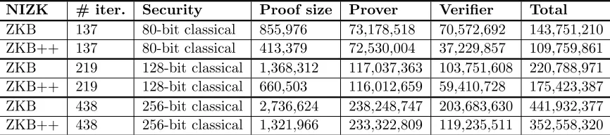
Table 1: Comparison of ZKB and ZKB++ proving knowledge of a SHA-256 preimage. The proof size is given in bytes, and the running times are given in CPU cycles. The running times are averages taken over 500 runs. The last two rows also target 128-bit PQ security. Only the Fiat-Shamir transform was used in this table.
5.1 Implementation and Benchmarks
We benchmarked ZKB++ and compared it to ZKB, and used it with LowMC to implement our signature scheme.
All of our code is written in C, and our benchmarks are taken on a desktop with a 4-core Intel Core i7-6700 3.40GHz CPU running Ubuntu 14.04. For the running time comparison, we compiled with GCC using the -O3 and -March=native flags for optimization. We give all of our running time benchmarks in units of CPU cycles.
The current benchmarks focus on signature size, since CPU cost is expected to be practical. In any case, neither our implementation, nor the one of Giacomelli et al. [10] is highly optimized. We plan to create a highly optimized implementation for one of our LowMC parameter sets. These optimizations should be independent of the FS or Unruh transform, since they will concentrate on the MPC component of ZKB++.
5.1.1 ZKB vs. ZKB++
In Table 1 we benchmark both the size and running times of ZKB++ and compare it to ZKB. Our proof size are more than a factor of 2 smaller, and we also saw increased running times – particularly for the verifier.
5.1.2 Signature scheme implementation
the signature scheme, our implementation allows one to “plug-in” any function they want without writing any code.
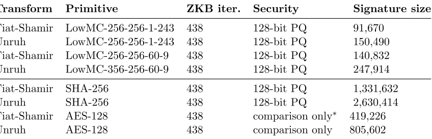
We benchmarked our implementation for AES and two configurations of LowMC. For the circuit files, we obtained an AES-circuit from [13].
In order to run our code with LowMC, we needed to obtain a binary circuit for it. As part of the ABY framework [8], circuit code was made available for LowMC. We began with that code and modified it to obtain compact circuits for the LowMC parameters that we benchmarked.
While the circuit-based implementation allows us to easily experiment with different functions for which we have circuit files, it suffers in efficiency since we are doing all of our operations as bitwise operations. We therefore created faster implementations for specific candidates, and we have benchmarked those here as well.∗
For each candidate, we show the results both using plain Fiat-Shamir, as well as using Unruh’s transformation. Note that, as expected, our modified Unruh scheme adds a fixed number of bytes that does not depend on the number of AND gates in the underlying symmetric function.
5.1.3 Parameters
For our post quantum choices, we targeted 128-bit post quantum security, and therefore chose our primitives to achieve 256-classical security. Based on Theorem 1, it was sufficient to have a block cipher with both a block size and a key size of 256. Moreover, for the base ZKB protocol, we need 256-bit classical soundness, and thus require 438 rounds based on our analysis in Section 4.2.1.
For LowMC, we require 256 bit blocks and cipher size. LowMC has two more parameters as well: data complexity and number of s-boxes. Given these parameters, we used the python script provided with the LowMC paper to determine the number of LowMC rounds required for security.
The data complexity parameter refers to the number of input/output pairs that an attacker will be given access to for a single key. In our signature scheme, the attacker only ever sees one such pair. However, in the simulation in the proof of Theorem 1, the attacker sees one more pair. Thus, the total data complexity is 2 pairs. In ZKB, the data complexity parameter is given as the base-2 logarithm of the number of pairs, and thus our data complexity is 1.
We were still free to choose the number of s-boxes. There is a signature size/efficiency trade-off since as we increase the number of s-boxes, the number of ANDs in the circuit increases, but the overall circuit size decreases. Thus, for our signature scheme, as we increase the number of s-boxes, the size of the signature will increase, but the time to sign and verify will decrease.
∗