Gene Expression with Pheonotype Classification
and Patient Survival Prediction Algorithm
1T.Shanmugavadivu,
M.C.A.,2Dr. T.Ravichandran, B.E (ECE), M.E(CSE), Ph.D., MISTE.,
1
Research Scholar, Karpagam University, Coimbatore - 641 021.
2
Dean, Department of ECE, SNS Engineering and Technology, Coimbatore-641 035.
Abstract: With more and more biological information generated, the most pressing task of bioinformatics has become to analyze and interpret various types of data, including nucleotide and amino acid sequences, protein structures, gene expression profiling and so on. We apply the data mining techniques of feature generation, feature selection, and feature integration with learning algorithms to tackle the problems of disease phenotype classification and patient survival prediction from gene expression profiles, and the problems of functional site prediction from DNA sequences. When dealing with problems arising from gene expression profiles, we propose a new feature selection process for identifying genes associated with disease phenotype classification or patient survival prediction. This method, GSA and GFA algorithms aims to select a set of sharply discriminating genes with little redundancy by combining entropy measure, Wilcoxon rank sum test and Pearson correlation coefficient test. In the study of patient survival prediction, we present a new idea of selecting informative training samples by defining long-term and short-term survivors. GFA is then applied to identify genes from these samples. A regression function built on the selected samples and genes by a linear kernel SVM is worked out to assign a risk score to each patient. In order to apply data mining methodology to identify functional sites in biological sequences, we first generate candidate features using k k-gram nucleotide acid or amino acid patterns and then transform original sequences respect to the new constructed feature space.
Keywords : Gene Selection Algorithm, Gene Filter Algorithm, Patient survival prediction Algorithm, Gene expression profile.
1.INTRODUCTION
The past few decades witness an explosive growth in biological information generated by the scientific community. This is caused by major advances in the field of molecular biology, coupled with advances in genomic technologies. In turn, the huge amount of genomic data generated not only leads to a demand on the computer science community to help store, organize and index the data, but also leads to a demand for specialized tools to view and analyze the data.
At the beginning, the main role of bioinformatics was to create and maintain databases to store biological information, such as nucleotide and amino acid sequences. With more and more data generated, nowadays, the most pressing task of bioinformatics has moved to analyze and interpret various types of data, including nucleotide and amino acid sequences, protein domains, protein structures and so on. To meet the new requirements arising from the new tasks, researchers in the field of bioinformatics are working on the development of new algorithms (mathematical formulas, statistical methods and etc) and software tools which are designed for assessing relationships among large data sets stored, such as methods to locate a gene within a sequence, predict protein structure and/or function, understand diseases at gene expression
level and etc. Motivated by the fast development of bioinformatics, this thesis is designed to apply data mining technologies to some biological data so that the relevant biological problems can be solved by computer programs. The aim of data mining is to automatically or semi-automatically discover hidden knowledge, unexpected patterns and new rules from data. There are a variety of technologies involved in the process of data mining, such as statistical analysis, modeling techniques and database technology. During the last ten years, data mining is undergoing very fast development both on techniques and applications. Its typical applications include market segmentation, customer profiling, fraud detection, (electricity) loading forecasting, and credit risk analysis and so on. In the current post-genome age, understanding floods of data in molecular biology brings great opportunities and big challenges to data mining researchers.
2. RELATED WORK
A Literature Review contains a critical analysis and the integration of information from a number of sources, as well as a consideration of any gaps in the literature and possibilities for future research. Feng Chu et al. [1] described their research in “Applications of Support Vector Machines to Cancer Classification with microarray data”. Microarrays also known as gene chips or DNA chips provide a convenient way of obtaining gene expression levels for a large number of genes simultaneously. Each spot on a microarray chip contains the clone of a gene from a tissue sample. Some mRNA samples are labelled with two different kinds of dyes, for example, Cy5 (red) and Cy3 (blue). After mRNA interact with the genes, i.e., hybridization, the color of each spot on the chip will change. The resulted image reflects the characteristics of the tissue at the molecular level. Microarrays can thus be used to help classify and predict different types of cancers. Traditional methods for diagnosis of cancers are mainly based on the morphological appearances of the cancers; however, sometimes it is extremely difficult to find clear distinctions between some types of cancers according to their appearances. Hence the microarray technology stands to provide a more quantitative means for cancer diagnosis. For example, gene expression data have been used to obtain good results in the classifications of lymphoma [2], leukemia [3], breast cancer [4] and liver cancer [5].
are usually very high dimensional. The dimensionality ranges from several thousands to over ten thousands. Second, gene expression data sets usually contain relatively small numbers of samples, e.g., a few tens. If we treat this pattern recognition problem with supervised machine learning approaches, we need to deal with the shortage of training samples and high dimensional input features. Recent approaches to solve this problem include artificial neural networks [7], an evolutionary algorithm [6], nearest shrunken centroids [6], and a graphical method [8]. In this paper, we applies a powerful classifier, i.e., the support vector machine (SVM), and four effective feature reduction methods, i.e., principal components analysis (PCA), class-separability measure, Fisher ratio, and t-test, to the problem of cancer classification based on gene expression data.
Brown et.al [9] introduced a new method of functionally classifying genes using gene expression data from DNA microarray hybridization experiments. The method is based on the theory of support vector machines (SVMs). Brown et.al described SVMs that use different similarity metrics including a simple dot product of gene expression vectors, polynomial versions of the dot product, and a radial basis function. Compared to the other SVM similarity metrics, the radial basis function SVM appears to provide superior performance in identifying sets of genes with a common function using expression data. In addition, SVM performance is compared to four standard machine learning algorithms. SVMs have many features that make them attractive for gene expression analysis, including their flexibility in choosing a similarity function, sparseness of solution when dealing with large data sets, the ability to handle large feature spaces, and the ability to identify outliers.
3. FEATURE SELECTION TECHNIQUE
Feature selection techniques can be categorized according to a number of criteria. One popular categorization is based on whether the target classification algorithm will be used during the process of feature evaluation. A feature selection method, that makes an independent assessment only based on general characteristics of the data, is named “filter” while, on the other hand, if a method evaluates features based on accuracy estimates provided by certain learning algorithm which will ultimately be employed for classification, it will be named as “wrapper”. With wrapper methods, the performance of a feature subset is measured in terms of the learning algorithm’s classification performance using just those features. The classification performance is estimated using the normal procedure of cross validation, or the bootstrap estimator. Thus, the entire feature selection process is rather computation-intensive. For example, if each evaluation involves a 10-fold cross validation, the classification procedure will be executed 10 times. For this reason, wrappers do not scale well to data sets containing many features. Besides, wrappers have to be re-run when switching from one classification algorithm to another. In contrast to wrapper methods, filters operate independently of any learning algorithm and the features selected can be applied to any learning algorithm at the classification stage.
Filters have been proven to be much faster than wrappers and hence, can be applied to data sets with many features. Since the biological data sets often contain a huge number of features (e.g. gene expression profiles), we concentrate on filter methods. Another taxonomy of feature selection techniques is to separate algorithms evaluating the worth or merit of a subset features from those of individual features. Correlation-based feature selection is a method that assesses and selects a subset of features. Gene Filter Algorithm (GFA) which first evaluates features individually and then forms the final representative feature set by considering the correlations between the features.
4. GENE FILTER (GFA)AND GENE SELECTION (GSA) ALGORITHMS
Gene Filter Algorithm GFA is a new strategy to conduct feature selection, mainly aiming to find significant genes in supervised learning from gene expression data. In this algorithm, we combine the above presented methods of entropy measure and Wilcoxon rank sum test, as well as Pearson correlation coefficient test together to form a three-phase feature selection process. In three-phase I, we apply Fayyad’s entropy-based discretization algorithm described in to all the numeric features. We will discard a feature, if the algorithm cannot find a suitable cut point to split the feature’s value range. One point needs to be emphasized here is that we will use numeric features all the way, though a discretization algorithm is involved to filter out some features in this phase.
In phase II, we conduct Wilcoxon rank sum test only on features output from phase I. For a feature f, the test statistical measure can be calculated by the way. If w(f) falls outside the interval [clower, cupper] where clower and cupper are the lower and upper critical test values. We will reject the null hypothesis and this indicates that the values of feature fare significantly different between samples in different classes. In the calculation of the two critical values clower and cupper, the standard 5% or 1% significant level is generally used. Therefore, by this phase, we is left with two groups of features: one group contains features f1 such that w(f1) < clower, the other group contains features f2 such that w(f2) > cupper. Features in same group are supposed to have similar behavior - having relatively larger values in one class of samples and relatively smaller values in another class of samples. In a gene expression data analysis, it is of a great interest to find which genes are highly expressed in a special type of samples (such as tumor samples, or patients with certain disease).
Step-1: k=1
Step-2: Rank all feature in group F on class entropy in an ascending order, f1,f2,….f1.
Step-3: Let Sk={f1} and remove f1 from F. Step-4: For each fi(i > 1)
Calculate Pearson correlation coefficient r(f1,fi); If r(f1, fi ) > rc
Add fi into Sk and remove it from F; Step-5: k=k+1 and goto step 2 until F=Φ.
In phase III, for each group of features, we examine correlations of features within the group. For those features that are in the same group and are highly correlated, we select only some representatives of them to form the final feature set. In gene expression study, high correlation between two genes can be a hint that the two genes belong to the same pathway, are co-expressed or are coming from the same chromosome. “In general, we expect high correlation to have a meaningful biological explanation. If, e.g. genes A and B are in the same pathway, it could be that they have similar regulation and therefore similar expression profiles”. We proposes to use more uncorrelated genes for classification since if we has lots of genes from one pathway, the classification result might be skewed.
Step-1: Select a statistic which will be used to measure differences between classes.
Step-2: Determine the threshold of the statistic according to significant level α.
Step-3: Calculate the test statistic for each of total features Step-4: Get the number of features selected by the
threshold record as w.
Step-5: For ith permutation test iteration (i=1,2…….,t):generate a pseudo data set by randomly permuting the class labels of all the samples, calculate the same test statistic for every feature, record how many features are selected by the threshold ,denote it as ki.
Step-6: Compute the percentage of features selected during the permutation test,
p=
1
t i i
k
t m
calculate p×w to be the expected number of false positive
Figure-2: Gene Selection Algorithm (GSA)
Using GSA, in gene expression data analyses where there are often more than thousands of features, we expect to identify of a subset of sharply discriminating features with little redundancy. The entropy measure is effective for identifying discriminating features. After narrowing down by the Wilcoxon rank some test, the remaining features become sharply discriminating. Then, with the correlation examination, some highly correlated features are removed to reduce redundancy. We does not use CFS in Phase III of GSA, because CFS sometimes returns too few features to comprehensively understand the data set. For example, CFS selects only one feature if the class entropy of this feature is zero. However, Pearson correlation coefficient also has a shortcoming - the calculation of correlation is dependent on the real values of features - it is sensitive to some data transformation operations. Therefore, other algorithms are being implemented to group correlated features.
5. PATIENT SURVIVAL PREDICTION ALGORITHM Step-1 : Read n samples.
Step-2 : Select training samples.
Step-3 : If training samples long-term and short term then
Step-4 : Identify genes
Step-5 : Genes related to survival
Step-6 : Build SVM scoring function and form risk groups
Step-7 : Assign risk score and risk group to each sample
Step- 8 : Draw Kaplan–Meler curves
Figure-3 : Patient Survival Prediction Algorithm
One of the main features of our new method is to select informative training samples. Since we focus is on the relationship between gene expression and survival, the survival time associated with each sample plays an important role here - two types of extreme cases, patients who died in a short period (termed as “short-term survivors”) and who were alive after a long period (termed as “long-term survivors”), should be more valuable than those in the “middle” status. Thus, We uses only a part of samples in training and this is clearly different from other approaches that use all training samples.
Formally, for a sample T, if its follow-up time is F(T)and its status at the end of follow-up time is E(T), then
Short - term survivor, if F(T)<c1 Λ
T is Long - term survivor, if F(T)>c2 Others, otherwise
After choosing informative training samples, we apply GFA and GSA algorithm to them to identify genes most associated with survival status. With the selected samples and genes, in the next step, we will build a scoring function to estimate the survival risk for every patient.
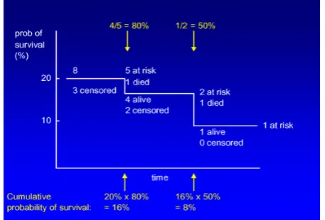
Kaplan-Meier analysis estimates a population survival curve from a set of samples. A survival curve illustrates the fraction (or percentage) survival at each time. Since in realistic clinical trial it often takes several years to accumulate the patients for the trial, patients being followed for survival will have different starting times. Then the patients will have various length of follow-up time when the results are analyzed at one time. Therefore, the survival curve cannot be estimated simply by calculating the fraction surviving at each time. For example, in the following study of lung adenocarcinomas, the patient’s follow-up time is varying from 1.5 months to 110.6 months. A Kaplan-Meier analysis allows estimation of survival over time, even when patients drop out or are studied for different lengths of time. For example, an alive patient with 3 years follow-up time should contribute to the survival data for the first three years of the curve, but not to the part of the curve after that. Thus, this patient should be mathematically removed from the curve at the end of 3 years follow-up time and this is called “censoring” the patient.
Figure 4 (a): Samples of Kaplan-Meier survival curves. It
is an example of a Kaplan-Meier survival curve. This group of patients has a minimum follow-up of a little over a year.
Figure 4(b): It is an illustration on how to calculate the
fraction of survival at a time.
On a Kaplan-Meier survival curve, when a patient is censored, the curve does not take a step down as it does when a patient dies; instead, a tick mark is generally used to indicate where a patient is censored and each death case after that point will cause a little bit larger step down on the curve. An alternative way to indicate a censored patient is to show the number of remaining cases “at risk” at several time points. Patients who have been censored or died before the time point are not counted as “at risk”. In Figure 4 (a) shows a complete sample of Kaplan-Meier survival curve with a tick mark representing a censored patient (captured from http://www.cancerguide.org/scurve_km.html), while Figure 4 (b) illustrates how to calculate the fraction of survival at a time.
To compare the survival characteristics between different risk groups for our survival prediction study, we draw Kaplan-Meier survival curves of the risk groups in one picture and use logrank test to compare the curves. The logrank test generates a p-value testing the null hypothesis that the survival curves are no difference between two groups. The meaning of p-value is that “if the null hypothesis is true, what is the probability of randomly selecting samples whose survival curves are different from those actually obtained”.
6. SIMULATION RESULTS
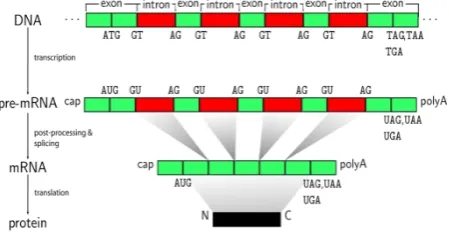
All biomedical data contain explicit signals or features as those in the classification problems raised by gene expression profiling. For example, DNA sequences and protein sequences represent the spectrum of biomedical data that possess no explicit features. Generally, a genomic sequence is just a string consisting of the letters “A”, “C”, “G”, and “T” in a “random order”. DNA process can be divided into two stages: transcription and translation.
Transcription: In this stage, the information in
DNA is passed on to RNA. This takes place when one strand of the DNA double helix is used as a template by the RNA polymerase to create a messenger RNA (mRNA). Then this mRNA moves from the nucleus to the cytoplasm. In fact, in the cell nucleus, the DNA with all the exons and introns of the gene is first transcribed into a complementary RNA copy named “nuclear RNA” (nRNA). This is indicated as “primary transcription” shown in Figure 6.1. Secondly, non-coding sequences of base pairs (introns) are eliminated from the coding sequences (exons) by RNA splicing. The resulting mRNA is the edited sequence of nRNA after splicing. The coding mRNA sequence can be described in terms of a unit of three nucleotides called a codon.
Translation: In this stage, the information that
in mRNA to form base pairs with the anticodon of another tRNA molecule. Hence, with the ribosome moving from codon to codon along the mRNA, amino acids are added one by one, translated into polypeptide sequences. At the end, the newly formed strand of amino acids (complete polypeptide) is released from the ribosome when a release factor binds to the stop codon. This is the termination phase of translation.
Figure 5: Process of protein synthesis
The functional sites in DNA sequences include transcription start site (TSS), translation initiation site (TIS), coding region, splice site, polyadenylation (cleavage) site and so on that are associated with the primary structure of genes. Recognition of these biological functional sites in a genomic sequence is an important bioinformatics application. We proposes a 3-step work flow as follows. In the first step, candidate features are generated using k-gram nucleotide acid or amino acid patterns and then sequence data are transformed with respect to the newly generated feature space. In the second step, a small number of good features are selected by a certain algorithm. In the third step, a classification model is built to recognize the functional site.
We generate the new feature space using k-gram (k=1, 2, 3…..) nucleotide or amino acid patterns. A k-gram is simply a pattern of k consecutive letters, which can be amino acid symbols or nucleic symbols. We uses each k-gram nucleotide or amino acid pattern as a new feature. For example, nucleotide acid pattern “TCG” is a 3-gram pattern while amino acid pattern “AR” is a 2-gram pattern constituted by an alanine followed by an arginine. We aim is to recognize functional site in a sequence by analyzing k-gram patterns around it. Generally, upstream and down-stream k-gram patterns of a candidate functional site (for example, every ATG is a candidate of translation initiation site) are treated as different features. Therefore, if we use nucleotide patterns, for each k, there are 2×4k possible combinations of k-gram patterns; if we use amino acid patterns, since there are 20 standard amino acids plus 1 stop codon symbol, there are 2×21k possible k-gram patterns for each k. If the position of each k-gram pattern in the sequence fragment is also considered, then the number of features will increase dramatically. We call these features as position-specific k-gram patterns. Besides, k-gram can also be restricted those in-frame ones.
The transformation is constructed as follows. Given a DNA nucleotide sequence, a sequence window is
set aside for each candidate functional site with it in the center and certain bases up-stream (named as up-stream window size) and certain bases down-stream (named as down-stream window size). If a candidate functional site does not have enough up-stream or down-stream context, we pad the missing context with the appropriate number of don’t-care (“?”) symbols.
If features are made from amino acid patterns, we will code every triplet nucleotides, at both up-stream and down-stream of the centered candidate functional site in a sequence window, into an amino acid using the standard codon table. A triplet that corresponds to a stop codon is translated into a special “stop” symbol. Thus, every nucleotide sequence window is coded into another sequence consisting of amino acid symbols and “stop” symbol. Then the nucleotide or amino acid sequences are converted into frequency sequence data under the description of our new features. Later, the classification model will be applied to the frequency sequence data, rather than the original cDNA sequence data or the intermediate amino acid sequence data.
In most cases, the number of candidate features in the feature space is relatively big. It is reasonable to expect that some of the generated features would be irrelevant to our prediction problem while others are indeed good signals to identify the functional site. Thus, in the second step, feature selection is applied to the feature space to find those signals most likely to help in distinguishing the true functional site from a large number of candidates. Besides, feature selection also greatly speeds up the classification and prediction process, especially when the number of samples is large. As used in gene expression data analysis (with name “all-entropy”), we choose all the features whose value range can be partitioned into intervals by Fayyad’s discretization algorithm. To achieve the ultimate goal of predicting the true functional site, we next step is to integrate the selected features by a classification algorithm. At this step, in the following two applications, we will focus on the results achieved by support vector machines (SVM) (with linear or quadratic polynomial kernel function).
7. CONCLUSION
tests. Compared with SVM, decision tree methods can provide simple, comprehensive rules and are not very sensitive to feature selections. Among the decision tree methods, the newly implemented CS4 achieves good prediction performance and provides many interesting rules.
Feature generation is important for some kinds of biological data. We illustrate this point by properly constructing new feature space for functional sites recognition in DNA sequences. Some of the signal patterns identified from the generated feature space is highly consistent with related literature or biological knowledge. The rest might be useful for biologists to conduct further analysis.
REFERENCES
1. A. A. Alizadeh, M. B. Eisen, R. E. Davis, C. Ma and I. S. Lossos et al., Distinct types of diffuse large b-cell lymphoma identified by gene expression profiling, Nature 403 (2000) 503–511.
2. T. Golub, D. K. Slonim, P. Tamayo, C. Huard and M. Gaasenbeek et al., Molecular classification of cancer: class discovery and class prediction by gene expression monitoring, Science 286 (1999) 531– 536.
3. X. J. Ma, R. Salunga, J. T. Tuggle, J. Gaudet and E. Enright et al., Gene expression profiles of human breast cancer progression, in Proc. Natl. Acad. Sci. USA, Vol. 100 (2003), pp. 5974–5979. 4. X. Chen, S. T. Cheung, S. So, S. T. Fan and C. Barry, Gene
expression patterns in human liver cancers, Molecular Biology of Cell 13 (2002) 1929–1939.
5. J. Khan, J. S. Wei, M. Ringner, L. H. Saal and M. Ladanyi et al., Classification and diagnostic prediction of cancers using gene expression profiling and artificial neural networks, Nature Medicine 7 (2001) 673–679.
6. J. M. Deutsch, Evolutionary algorithms for finding optimal gene sets in microarray prediction, Bioinformatics 19 (2003) 45–52.
7. R. Tibshirani, T. Hastie, B. Narashiman and G. Chu, Diagnosis of multiple cancer types by shrunken centroids of gene expression, in Proc. Natl. Acad. Sci. USA, Vol. 99 (2002), pp. 6567–6572. 8. E. Bura and R. M. Pfeiffer, Graphical methods for class prediction
using dimension reduction techniques on DNA microarray data, Bioinformatics 19 (2003) 1252–1258.
9. Feng Chu and Lipo Wang. Applications of Support Vector Machines to Cancer Classification with Microarray data. International Journal of Neural Systems, vol. 15, no. 6 (2005) 475–484.
10. Michael P. S. Brown,William Noble Grundy, David Lin, Nello Cristianini, and Charles Sugnet. Support Vector Machine Classification of Microarray Gene Expression Data. UCSC-CRL-99-09.
11. H.Witten and E. Frank. Data Mining: Practical Machine Learning Tools and Techniques with Java Implementation. Morgan Kaufmann, San Mateo, CA, 2000.
12. C.J. Thornton. Techniques in Computational Learning. Chapman and Hall, London,1992.
13. T.M. Mitchell. Machine Learning. McGrawHill, USA, 1997. 14. T. R. Golub, D. K. Slonim, P. Tamayo, C. Huard, M. Gaasenbeek, J.
P.Mesirov, H. Coller,M. L. Loh, J. Downing, M. A. Caligiuri, C. D. Bloomfield, and E. S Lander. Molecular classification of cancer: Class discovery and class prediction by gene expression monitoring. Science, 286:531–537, 1999.
15. M.A. Hall. Correlation-based feature selection for machine learning. PhD thesis, Department of Computer Science, University of Waikato, Hamilto, New Zealand, 1998.
16. V.N. Vapnik. The Natural of Statistical Learning Theory. Springer, 1995.
17. C.J.C. Burges. A tutorial on support vector machines for pattern recognition. DataMining and Knowledge Discovery, 2(2):121–167, 1998.