The Mathematical Model of the Movement of Heavy Objects in the Water

!

"!"

# $ $"

%

&

''' (

The Mathematical Model of the Movement of Heavy Objects in the Water

Li Yong*

College of Science, Guilin University of Technology

Guilin , P. R. China [email protected]

SHEN Xiao-kui

College of Science, Guilin University of Technology

Guilin , P. R. China

WANG Jun

College of Science, Guilin University of Technology

Guilin , P. R. China

Abstract:Based on the practical problems of breach closure, this paper studies the movement of heavy objects in the water. For questions 1 and 2, it establishes suitable models respectively. And for all data, it establishes the model 3. Moreover, this paper makes error analysis on the three models respectively. The results show that the models have a good fitting result and better theoretical.

Key words:Control variables; Bernoulli's equation; Newton iteration

I. RESTATEMENT OF THE PROBLEM

Based on the practical problems of using heavy objects for breach closure, this paper will study the movement of heavy objects in the water. The issue can be seen in the question of B at the Seventh National Graduate Mathematical Contest in Modeling.

II. MODEL ASSUMPTIONS

A. Thickness of the experimental tank glass is negligible; B. The water is non-sticky and incompressible liquid; C. The movement of objects ignores the roll in the water; D. The tank bottom is used as zero-potential surface in the

experiment.

III. SYMBOLS

Symbols Instructions

r

_{the density of water}

g

_{the gravitational field strength}

m

the mass of the object

bottom

s

the area that cross-sectioned by water surface of the object

( )

D

s t

the area of the region that formed from projection

D

of the object to

flow direction in the cross section

s

Ù _{the area that formed from projection of the object to face the flow surface}

( )

l t

the distance between the bottom and the surface of the object

k

the width that formed from projection of the object to face the flow

surface

H

the distance between the planes where the highest point and the lowest

point of the object are

y

the vertical axis of the center of gravity when the object put(the time 0)

V

Ù the volume of the object

( )

V t

the volume of the object into the water

IV. DATE PROCESSING

In the experiment, the region of the scales is outside of the glass tank. As the refraction of the water and glass medium, the coordinates of the movement of the observed object in the water must be translated. Here we ignore the thickness of the glass that is we ignore the refraction of light in the glass and only consider the refraction of light in the water. The distance between the center of the camera lens and the region of scale is 1.2m. When we observe the region of scale from the camera lens, the observed data also needs to be translated because of the existence of perspective. Therefore, the experimental observed data need to be translated if we want to get the true trajectory of the movement of object in the water.

Figure.1 the plan that determined by the incident light and refraction light

While,

n

₁is the refractive index of water and

n

₂is the refractive index of air. By the law of refraction:

1

sin

2

sin

n

a

=

n

b

So,

1

2 2 2 2

1 1 2 1 2

1 1

2 2 2 1

2 _{1 1} 2 1

2 2 2 1 2

(

)

sin

sin

(

)

s

s

h

s

s

h

n

s

s s

n

s

h

s s

s

s

h

b

a

+

-

+

=

=

=

×

-

+

--

+

(1) (1) square both sides, then we get:

2 2

2 2 2 1

2

1 1 1

2

2 1

( )

1

h

s

s

n

s

h

n

s

=

+

+

×

-Some point, the coordinate of the object in the plane of

scale is

B

( , )

x y

, the projection coordinate of the original

image point in the plane of scale is

A

( ', ')

x y

, the front

projection coordinate of the camera in the plane of scale

is

C

( , )

x y

_{0 0} .

Figure.2 position relationship of A B C

By the geometry of similar triangles:

0 0 2

0 0 1

'

'

x

x

y

y

s

x

x

y

y

s

-

-=

=

-

-

We can get the relationship of the front projection coordinate and preimage in the plane of scale is:

2 2

0 0

2 2 2 2 2 2

0 0 1 2 1 1

2 2

0 0

2 2 2 2 2 2

0 0 1 2 1 1

' (

1) (

)

((

) (

) )(

)

' (

1) (

)

((

) (

) )(

)

h n

x

x x

x

x x

y y

n

n

n h

h n

y

y y

y

x x

y y

n

n

n h

ì

=

+ × -

+

ï

ï

-

+ -

-

+

ï

í

ï =

+ × -

+

ï

-

+ -

-

+

ïî

V. MODEL ANALYSIS

A. Overview and Analysis About the Forces of Objects in the fluid

The factors that impact the forces of objects in the fluid are complex. One of the factors is block shape, but currently, it’s lack of the formula which used to calculate. In

y axis

-o

x

A

C B

'

y

y

0

y

0

x

'

x

2

s

1

s

B

β

C

α s1

2

s

1

h

A

2

applications, we often indirectly considered by using comprehensive coefficient [1]_{. It’s rarely described about the}

drag force changing with objects’ own scale, other objects around, relative position between objects and so on. The model in this article discusses the relationship between the joint force of flow that objects suffers and block shape, speed of flow and so on.

The interaction between fluids and objects is an important issue in fluid dynamics and applied in many fields. The complexity of the fluid itself and the diversity shape of the object both determine the complexity of the study. In this model, for considering the solvability of differential equations and the feasibility of the model, we ignore the flow separation, vortex caused by the changes of fluid flow around the object.

Generally, the force acting on an object can be divided into the following categories [2]_:

[a] The force that independent from the relative motion of fluid-objects (Even if the relative velocity and acceleration is zero, this force does not disappear). Such as inertia, gravity and pressure forces, etc; [b] The relative motion depends on fluid-objects, the force

whose direction of relative motion along the direction is the longitudinal force. For example, drag force, added mass force, Basset force and so on;

[c] The relative motion depends on fluid-objects, the force whose direction perpendicular to the direction of relative movement is the lateral force. For example, the lift force, Magnus force, Saffman force and so on.

The pressure difference in the first category, all of the second and third category powers are called white power.

The next, we will analyze these given common forces that combine this model:

[a] Gravity is the gravitational force between objects with the Earth.

[b] If the pressure gradient is caused by gravity of fluid, corresponding pressure difference is the buoyancy, also called the generalized buoyancy. This paper considers separately the impact of buoyancy on the object, do not merge for the underwater gravity or effective gravity.

[c] Added mass force is object to the acceleration a(t) for accelerated motion in a fluid when the fluid is bound to drive around some of the force accelerate the director of health. Application of the ideal (non-viscous) fluid dynamics theory, this effect is equivalent to the object has an additional quality. This

ignores the added mass.

[d] Since the presence of viscous fluid, the speed changes when the object, that object has a relatively acceleration, the flow field around the object cannot be immediately reached stability. Therefore, the fluid force on the particles depend not only on the relative velocity of the object at the time (some resistance), and then the relative acceleration (added mass force), but also on the acceleration of history in the past, this part of the force called Basest force. We consider the ideal fluid, regardless of Basest force.

[e] If the object rotate by the angular velocity

w

and rotation axis perpendicular to the relative velocity, the object not only by a vertical resistance. But also by the relative speed and a vertical axis of rotation in the lateral force, the direction of relative velocity and angular velocity into the right system, this phenomenon is the Magnus effect [3], and Magnus force is the force generated.

[f] If the flow field has velocity gradient, the object will suffer an additional lateral force, and this is the Saffman force.

[g] The common formula we use to calculate the drag force is applying Evett’s [4]_,

1

₁ 2

2

D D

F

=

r

C AU

While,

C

_Dis drag coefficient;

U

is mean vertical

velocity;

A

₁is the area that formed from projection of the object perpendicular to flow direction.

[h] For non-spherical massive object, Literature [5] _shows

that value of the uplift force is very small and close to zero, so this is not considered.

[i] Bingham flow shear stress: When the water in the sediment is high, especially it has higher levels of cohesive particles, it can be regarded as Bingham [6]_.

The model experiment is carried out in water, so the stress is not considered.

[j] Adhesion and thin film of water: we consider it when study the fine sediment but ignore it when study large objects [7]_.

force and so on. Thus, we can seize the main factors, ignore secondary effects and establish the ideal and yet precise model of the movement of objects in the ideal fluid.

Define a

t

,

t

_b and

t

_care the time when the object just

touches the water, full accesses to the water, and contacts the bottom of the tank respectively. Corresponding,

0

®

t

a is called the process of the object moving in the air,

a b

t

®

t

is called the process of the object into the water,

b c

t

®

t

is called the process of the object moving in the

water. Each process is divided into horizontal direction (x) and vertical direction (y). The end speed of a process determines the initial speed of the next process. To highlight that not all test

objects has the process of the object moving in the air. For example, the test about an object with the center of gravity on the surface of the water, at this point, we’ll start from the newly recruited water.

B. Modeling to Problem 1

[a] The Motion Analysis of the Large Solid Cube Before Entering the Water

While

t

Î

(0, )

t

_a , we launch the large solid cube

vertically. At this moment, the initial velocity of the cube is 0 and in the vertical direction, the cube is on free fall. So the rate equation is expressed as ( ) 0

( )

x y

v t

v t g t

ì =

ï

í ₌

ïî

. While

t

_a, the

vertical coordinates of the center of gravity of the cube

is

( )

_{0 0}t

( )

27.5

2

a

a y

H

y t

=

y

-

ò

v

q

d

q

=

+

, then

0

2 55 H

a

y t

g

-

-= and the speed at time

t

a

is

0

( ) 0

( )

(2

55 H)

x a

y a

v t

v t

y

g

ì

=

ï

í

=

-

-ïî

.

[b] The Motion Analysis of the large solid cube Entering the Water

[i] The Motion Analysis in the Vertical Direction

While

t

Î

( , )

t t

_{a b} ,we do the force analysis on the large

solid cube. In the vertical direction, it suffers the gravity

G

which is constant in direction and size as well as

the buoyancy

F t

_b

( )

which is constant in direction but

mutative in size. Take straight down as the positive direction, then the cube suffers the total force is:

( )

( )

( )

( )

f b bottom

F t

= -

G F t

=

mg

-

r

gV t

=

mg

-

r

gs

l t

(2)

In the process, the speed of the cube at any

t

time is:

( )

( )

y

d l t

v

t

d t

=

(3)

Then:

( )

( )

a t

y t

l t

=

ò

v

q

d

q

(4) The acceleration at

t

time is:

( )

( )

y

y

d v

t

a

t

d t

=

(5)

Figure.3 Schematic diagram of the process of the object into the water According to Newton's second law:

b

F

A B

water surface

time

t

_a time

t

time

t

_b

f

F

=

ma

(6)

By (2),(5),(6), we get:

( )

( )

( )

( )

y b bottom

y

dv t

F t

gs

l t

a t

g

g

dt

m

m

r

=

= -

= -

(7)

( )

y

v t

is determined by (3) and (7).

[ii] The Motion Analysis in the Horizontal Direction

The force on the large solid cube in the horizontal direction is very complex, so we build ideal model. Take the right level as the positive direction. We select two

point

A,B

from the left and right side of the cube (seen in

fig.3). Supposing the pressure of

A,B

are

p t p t

_A

( ),

_B

( )

,

the height of

A,B

are

h h

_A

,

_B. We consider the water velocity facing the water is equal to the motion speed of object and the water velocity backing the water is equal to the controlled speed of the water tank.

The Bernoulli’s equation on the two points

A,B

is:

2

2

1

( )

( )

2

1

( )

2

A A x

B B water

p

t

gh

v

t

C

p

t

gh

v

C

r

r

r

r

ì

+

+

=

ï

ï

í

ï

+

+

=

ï

î

And the solution is:

2

2

1

( )

( )

2

1

( )

2

A A x

B B w a t e r

p

t

C

g h

v

t

p

t

C

g h

v

r

r

r

r

ì

=

-

-ï

ï

í

ï

=

-

-ï

î

(8) Then in the horizontal direction, the cube suffers the total force is:

2 2 2 2

1 1 1

( ( )) ( ) ( ( )) ( )

2 2 2

x A x B water water x D

D D

F=

òò

C-rgh- rv t ds-

òò

C-rgh- rv ds= rv -v t s t

(9) By the Newton’s second law

F

_x

=

ma t

_x

( )

, (9) can change into:

2 2

1

(

( )) ( )

2

x

water x D

dv

v

v

t s t

m

dt

r

-

=

(10)

By (10) and

s

_D

( )

t

=

kl t

( )

, we can determine the

curve of horizontal velocity that changes with time.

C. The Motion Analysis of the Large Solid Cube Completely in the Water

When surface of the object leave the water surface, that is the object is completely in the water just at

time

t

Î

( , )

t t

_{b c} ,

s

_D

( )

t

reach the maximum

s

_D Ù

. Therefore,

after slightly modifying the equation for the process of entering the water, we can get the equation of motion in the water.

D. Analysis of Problem 2

Question 1 is the promotion of question 2. As to question 2, functional relation of geometric characteristic quantity of the object is very complex (for example, when we erect hollow tiles into the water, functional relation of the volume and height into the water must be divided into three parts to express). So, for the built model being general, we regard the object as particle and ignore the process of entering the water. What’s more, according to numerical calculations of model 1, we can see when focus of the large solid square is on the surface of the water, the whole process of being flat into the water is only 0.06s. Yet the contact area of the large cube into the water is the largest among all objects placed in any way. So the drag coefficient is the largest. And from the point of view of model 1, the time of other objects into the water is certainly less than 0.06s. Therefore, when we build model 2, we ignore the time of the object into the water. We’ll consider the whole movement as particle and this has little effect on the entire process.

The analysis method of the movement in the air and in the water is exactly the same to problem 1.

E. Analysis for the Given Date

[image:6.612.61.276.57.147.2] [image:6.612.317.554.433.691.2]

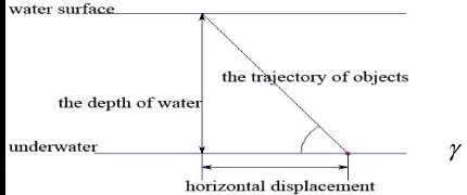
Figure.4 the trajectory of the object according to the simulation data

Figure 4 shows that if the depth of the water is known, the factor that affects the horizontal displacement is the angle

γ

. Therefore, we qualitatively analyze water speed, shape, size and other factors have impact on

γ

through the given data.

VI. MODELING

A. Modeling 1 for the Large Solid Square to Problem 1

The velocity equation of the movement of the square is:

1)

( ) 0

( )

x

y

v t

v t

gt

ì

=

ï

í

=

ïî

t

Î

(0, )

t

a

2) 2 2 1 ( ( )) ( ) 2 ( ) ( ) ( ) ( ) ( ) ( ) x

w ater x D

D

y bottom

y

d v

v v t s t m

d t s t kl t

d v t g s l t g

d t m

d l t v t d t r r ì - = ï ï ï ₌ ï ï í

ï =

-ï ï

ï ₌

ïî

t

Î

( , )

t

_a

t

_b

3) 2 2 1 ( ( )) 2 ( ) x water x D

y

dv

v v t s m

dt dv t

mg g V m

dt r r Ù Ù ì - = ï ï í ï - = ï î

t

Î

( , )

t

b

t

c

Coordinate equation of the movement of the square is:

t 0 t 0 ₀

( )

( )

( )

( )

x y

x t

v

d

y t

y

v

d

q

q

q

q

ì

=

ï

í

ï

=

-î

ò

ò

B. Modeling 2 to Problem 2

[a] Model of the movement of single object in the water The velocity equation of the movement is:

1) ( ) 0

( ) x

y v t v t g t

ì =

ï í

= ïî

_{t 0,} 2y0 5 5 g

æ _- ö

ç ÷

Î ç ÷

è ø 2) 2 2

1

(

( ))

2

( )

x

water x D

y

dv

v

v

t

s

m

dt

dv t

mg

g V

m

dt

r

r

Ù Ù

ì

-

=

ï

ï

í

ï

-

=

ï

î

0

2

55

,

c

y

t

t

g

æ

-

ö

ç

÷

Î ç

è

÷

ø

Coordinate equation of the movement is:

t 0 t 0 ₀ ( ) ( ) ( ) ( ) x y

x t v d

y t y v d

q q

q q

ì ₌

ï í

ï ₌

-î

ò

ò

[b] Model of the movement of the component which is formed by two objects’ connection in the water The expression about the velocity and coordinates equation of the model is same to the single’s. In calculating

the area

s

_D Ù

which is facing the flow, the original should be

multiplied by 2.

C. Modeling 3 for the Given Data

Since models 1 and 2 only consider a few factors on using of mathematical and physical methods, so we use small-scale test data to build model 3 related to 7 factors.

Build a generalized function

g j x x x x x x x

=

( , , , , , , )

_{1 2 3 4 5 6 7}

according to the given data. The function shows the angle of the rail line and the level in the state

of

( , , , , , , )

ξ ξ ξ ξ ξ ξ ξ

_{1 2 3 4 5 6 7} . Kinds of variables are defined as the follow table.

Table 1:

Variable Variable conditions

Symbol Instructions 1 2 3 4

1

ξ

water

velocity 34 40 47 55

2

ξ

release

height 0 5 12 -

3

ξ

shape cube honeycom

b cones -

4

ξ

delivery

method flat heel standing -

5

ξ

size small big - -

6

ξ

hollow solid hollow solid - -

7

ξ

connected or

not

not

connected connected - -

Note: "-"indicates that there is not defined.

For example,

ϕ

(2,3,1, 2,1,1, 2)

represents the angle of the rail line and the level, which is fit out by releasing of

two connected small hollow squares flatting on 12cm height of the water surface when the water velocity is 40m/s. We can calculate the angle

γ

of each set of experiments on using the least squares method.

VII. SOLUTION

A. Solution to Model 1

[a] The Process of the Object into the Water

In (7) derivative of

t

and combine (4): 2

2

( )

( )

y _{b otto m}

y

d v

t

g s

v

t

dt

m

r

= -

(11)

Solving (11), we can get:

2 3

( )

sin

bottom

(

)

y

gs

v t

c

t c

m

r

æ

ö

ç

÷

= ×

ç

+

÷

è

ø

(12)

Put (12) into (4):

2 3

( )

cos

bottom

(

)

ta

t bottom

gs

m

l t

c

c

gs

m

r

q

r

æ

ö

ç

÷

=

×

ç

+

÷

è

ø

(13)

Put(13) into (7):

y

()

₂ bottom

cos

bottom

(

₃

)

₂ bottom

cos

bottom

( )

₃ a

gs

dv t

gs

gs

gs

g c

t c

c

t c

dt

m

m

m

m

r

r

æ

ç

ö

÷

r

æ

ç

r

ö

÷

= -

×

ç

+ +

÷

×

ç

+

÷

ç

÷

è

ø

è

ø

(

2 3

( )

cos

(

)

y bottom bottom

dv t

gs

gs

c

t c

dt

m

m

r

æ

ç

r

ö

÷

=

×

ç

+

÷

è

ø

(15)

By (14) and (15):

2 bottom

cos

bottom

(

a 3

)

0

gs

gs

g

c

t

c

m

m

r

æ

ç

r

ö

÷

-

×

ç

+

÷

=

è

ø

(16)

By (12) and (16):

2 3

2 3

cos

(

)

( )

sin

bottom

(

)

bottom bottom

a

y a a

gs

gs

g

c

t

c

m

m

gs

v t

c

t

c

m

r

r

r

ì

æ

ö

ï

=

×

ç

+

÷

ï

ç

÷

è

ø

ï

í

æ

ö

ï

ç

÷

ï

= ×

ç

+

÷

ç

÷

ï

è

ø

î

(17)

Solution of (17):

2 2 3 ₂

( )

( )

arcsin

( )

y a bottom

bottom

bottom y a

a

bottom _{y a bottom}

v

t

s

mg

c

s

s

v t

m

c

t

gs

v

t

s

mg

r

r

r

r

r

ì

+

ï

=

ï

ï

í

ï

ï

=

-ï

+

î

Therefore, the velocity of the movement of the object in vertical is:

(18)

( ) ( )

D

s

t l t

,

can be solved by

v t

_y

( )

.

And

( )

2

₂

( )

₂

( )

x D

water x

dv t

s t dt

m

v

v

t

r

=

-

(19)

Solving (19), we can get:

4

2

( )

(

( ) )

exp

1

water x water water D

v

v t

v

v

c

s t dt

m

r

=

-æ

-

ö

ç

÷+

ç

÷

è

ø

ò

By the equation

v t

x

( ) 0

_a

=

, we can get the parameter

c

4. [b] The Movement of Objects in the Water

Similar to the process of entering the water, we can get the velocity function:

5 6

2

( )

(

)

exp

1

( )

w ater

x w ater

w ater D

y

v

v

t

v

v

c

s t

m

g V

v

t

g

t

c

m

r

r

Ù Ù

ì

=

-ï

æ

ö

ï

ç

-

÷

ï

ç

÷

+

ïï

ç

÷

è

ø

í

ï

æ

ö

ï

ç

÷

ï

=

ç

-

÷

+

ï

ç

÷

ï

è

ø

î

(20)

By the condition that the end speed of a process is the initial speed of the next process, we can get the

parameter

c c

₅

,

₆and determine the coordinate trajectory according to the coordinate equation.

B. Solution to Model 2

is

2

y

0

55

g

-, so:

0 7

2

0

2

55

exp

(

) 1

water water

water

D

v

v

v

y

c

s

m

r

g

Ù

-

=

æ

-

ö

ç

-

÷

+

ç

÷

è

ø

Then:

c

₇

s

_D

2

y

0

55

g

r

Ù

-=

The horizontal velocity is:

0

2

( )

2

55

exp

(

)

1

water

x water

water D

v

v t

v

v

y

s

t

m

r

g

Ù

=

æ

ö

-ç

-

÷

+

ç

÷

è

ø

(21)

The following we’ll discuss the trajectory of the object. From (21), we can get the horizontal coordinate of the

object

0 (2 55)/

( )

t _{y g} x

( )

x t

v

q

d

q

-=

ò

Solving the above equation, we can obtain:

Since the time characteristics of the given data is not obvious, that means the first line is the 0.04th_{s for starting}

sampling yet not necessarily the 0.04th_{s of the movement of}

the object. So we join the time calibration items

ε

_aand

displacement calibration items

ε

_b ,

thenx t( ) = x t( +e _a)+e _b .

Select the data of the two moments on

t t

₁

,

₂, then we can get

ε

_aand

ε

_b . However, the equation about

ε

_ais

0

x

e

+ =

x

and this type of equation has no way to obtain symbolic solutions. We can use Newton iteration to solve

the equation approximately.

Make

F

( )

e

_a

=

x

(

e

_a

+

t

₁

)

+

x

(

e

_a

+

t

₂

) (

-

x

₁

-

x

₂

) 0

=

, we can obtain

ε

_a ,then we can obtain

ε

_b . Establish

iterative ₁

( )

( )

n

n n

n

F x

x

x

F x

+

=

-

¢

, we can calculate the vertical

coordinate:

( )

6370

2 _{10 11}

23

y t

= -

t

+

c t c

+

.

We select the data on ideal moment

t t

₁

,

₂ in the experiment. The ideal moment here means that after the object is completely out of the surface of the water and before the object is about to contact the bottom. That is, excluding the data near the two critical moments. The aim is to try to simulate the process of movement of the object entirely in the water.

Thus,

2

1 1

11 1

2 2 10

2 2

6370

( )

1

23

1

6370

( )

23

y t

t

c

t

c

t

y t

t

æ

ö

ç

+

÷

æ

ö

æ

ö

ç

÷

=

ç

÷

ç

÷

ç

÷ ç

֍

÷

ç

+

÷ è

ø è

ø

ç

÷

è

ø

.With

experimental data, we can calculate the parameter

2

1 _{1 1}

1 1 1

2

1 0 2

2 2

6 3 7 0

( )

1

2 3

1

6 3 7 0

( )

2 3

y t

t

c

t

c

t

y t

t

-

æ

ç

+

ö

÷

æ

ö

æ

ö ç

÷

ç

÷

=

ç

ç

÷

÷

ç

÷

ç

÷

ç

÷

è

ø

è

ø

ç

+

÷

è

ø

to

determine

y t

( )

,

x t

( )

in the vertical direction.

We use the issue (2) raised by question 4 as an example on operation. When the object weighs 1.5t, the breach is 3m depth and the breach flow is 4m/s, we should throw ahead of 4.21304m. If the breach is 4m depth and the breach flow is 5m/s, we should throw ahead of 6.37126m. We don’t consider the stability of the object sink to the bottom. Objects sink to the bottom will be effective.

C. Analysis of Model 3

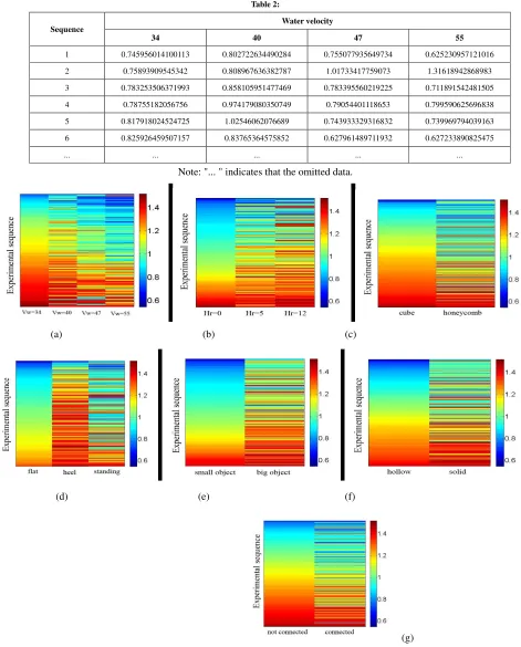
to 4 different column regions to distinguish between different gradient. And the different color-scale value reflects the size of

g

. The greater the scale value is, the greater

g

is; the smaller the scale value is, the smaller

g

is. In order to show better experimental results, we place the [image:9.612.62.533.128.713.2]

experimental sequence on the vertical axis after re-arranged in ascending. The form of the data can be seen in table 2. So the colors of part of the first column in fig.5 are uniform with a slow gradient.

Table 2:

Sequence

Water velocity

34 40 47 55

1 0.745956014100113 0.802722634490284 0.755077935649734 0.625230957121016

2 0.75893909545342 0.808967636382787 1.01733417759073 1.31618942868983

3 0.783253506371993 0.858105951477469 0.783395560219225 0.711891542481505

4 0.78755182056756 0.974179080350749 0.79054401118653 0.799590625696838

5 0.817918024524725 1.02546062076689 0.743933329316832 0.739969794039163

6 0.825926459507157 0.83765364575852 0.627961489711932 0.627233890825475

... ... ... ... ...

Note: "... " indicates that the omitted data.

(a) (b) (c)

(d) (e) (f)

(g)

By observing the graph, it follows the below rules in general:

(a) Fig.5(a) shows the greater the water velocity is,

g

is smaller;

(b) Fig.5(b) shows the greater the height is,

g

is greater; (c) Fig.5(c) shows the shape has no significant effect on

g

; (d)Fig.5(d) shows when heel,

g

is maximum; stand placed second and flat is minimum;

(e) Fig.5(e) shows the greater the volume of the object,

g

is smaller;

(f) Fig.5(f) shows when it’s hollow,

g

is small, but when it’s solid,

g

is great;

(g) Fig.5(g) shows it has no significant effect on

g

whether connection or not.

VIII. MODEL INSPECTING AND ERROR

ANALYSIS

A. Inspection of Model 1

[a] The Comparative Analysis of the Trajectory of Model 1 and the Actual

The comparison of the real trajectory of the large solid cube and simulated model 1 can be seen in fig.6.

(a)

(b)

(c)

(d)

(e)

(f)

Figure.6 the comparison of fitting curve of model 1 and the experimental

data

[b] Error Analysis

From the above simulation of the figure, we can see there are some errors in the curve of model 1 with the experimental data, especially the curve of the vertical axis changing with time. This phenomenon is mainly due to the movement of objects in the fluid is very complex. The force acting on an object is a lot and we cannot completely consider. But these forces will have some impact on the trajectory of the movement of objects. It is precisely because the model is built in the ideal fluid and ignores many factors, it still have large errors even taking into account the impact of inaccurate data. However, generally speaking, the simulated running track can still explain the trajectory of the object in the fluid. There is some value on analyzing it.

B. Inspection of Model 2

their real action. This method can be used to study all the tests.

[a] Error data of Model 2

We assume 0.001cm as an error gradient and make out the frequency distribution of average error of model 2(fig.7),

(a) (horizontal)

(b) (vertical)

Figure.7 the frequency distribution of average error of model 2

As can be seen from the figure, the error focus in 0~2.5cm. Therefore, errors in model 2 is relatively small and this shows the model 2 has a relatively strong theoretical.

[b] Error Analysis

As different shapes of a variety of objects, it is more difficult to analyze the changes of force in the process of the object into the water. We neglect the process from the new to enter the water in model 2, which is the main reason for generating errors.

IX. SUMMARY

This paper designs three different models according to the raised issues. Model 1 analyzes the movement of the object in three periods comprehensively. But when the shape of the object is irregular, it is difficult to simulate the process from the new to water to complete in the water. In model 2, we ignore the movement of the second period

because it is a short time for general object go into the water and it has little impact on the model. Thus model 2 is more widely used in the movement of various shapes of objects into the water. Model 3 controls the variables that may affect the rest of the model factors by control variables and only do qualitative analysis to one of these variables to understand the impact of various elements of the model. Experimental results show that this model has a good fitting effect and has a better theoretical. It has some reference value to study the problem of breach closure by heavy objects.

X. REFERENCES

[1] Qian Nin,Wan Zhao-hui Mechanics of

sediment[M].BeiJing: Science Press, 2003:114~122

[2] Liu Da-you, Wang Guang-qian, Li Hong-zhou Stress

Analysis of sediment movement- Discussion on the impact

force[J] Sediment Research ,1993(2):41~47

[3] Chen Yu-pu Fluid Dynamics [M] NanJing: Hehai

University Press ,1990:201~207

[4] Evett J B,and liu C Fundamentals of Fluid

Mechanics[M]New ork:McGraw-Hill 1987:381~390

[5] Zhu L J,wang J Z,Cheng N S,Ying Q,and Zhang D

F Setting Distance and incipient motion of sandbags in

open channel flows[J] Waterway, Port, Coastal and Ocean

Eng, ASCE,2004,130(2):98~103

[6] Luo Wen-feng , Ai Nan-shan, Ding Jin, etc Bingham

flow in the management of sediment Starter[J] Journal of

Hydraulic Engineering 2000(12),64~67

[7] Du Guo-ren On incipient velocity of