Combining Utterance-Boundary and Predictability Approaches to
Speech Segmentation
Aris XANTHOS
Linguistics Department, University of Lausanne UNIL - BFSH2
1015 Lausanne Switzerland [email protected]
Abstract
This paper investigates two approaches to speech segmentation based on different heuris-tics: the utterance-boundary strategy, and the predictability strategy. On the basis of for-mer empirical results as well as theoretical con-siderations, it is suggested that the utterance-boundary approach could be used as a prepro-cessing step in order to lighten the task of the predictability approach, without damaging the resulting segmentation. This intuition leads to the formulation of an explicit model, which is empirically evaluated for a task of word segmen-tation on a child-oriented phonemically tran-scribed French corpus. The results show that the hybrid algorithm outperforms its compo-nent parts while reducing the total memory load involved.
1 Introduction
The design of speech segmentation1 methods has been much studied ever since Harris’ sem-inal propositions (1955). Research conducted since the mid 1990’s by cognitive scientists (Brent and Cartwright, 1996; Saffran et al., 1996) has established it as a paradigm of its own in the field of computational models of language acquisition.
In this paper, we investigate two boundary-based approaches to speech segmentation. Such methods “attempt to identify individual word-boundaries in the input, without reference to words per se” (Brent and Cartwright, 1996). The first approach we discuss relies on the utterance-boundary strategy, which consists in reusing the information provided by the occur-rence of specific phoneme sequences at utter-ance beginnings or endings in order to
hypoth-1
To avoid a latent ambiguity, it should be stated that
speech segmentationrefers here to a process taking as in-put a sequence of symbols (usually phonemes) and pro-ducing as output a sequence of higher-level units (usually words).
esize boundaries inside utterances (Aslin et al., 1996; Christiansen et al., 1998; Xanthos, 2004). The second approach is based on the predictabil-ity strategy, which assumes that speech should be segmented at locations where some mea-sure of the uncertainty about the next symbol (phoneme or syllable for instance) is high (Har-ris, 1955; Gammon, 1969; Saffran et al., 1996; Hutchens and Adler, 1998; Xanthos, 2003).
Our implementation of the utterance-boundary strategy is based on n-grams statistics. It was previously found to perform a “safe” word segmentation, that is with a rather high precision, but also too conser-vative as witnessed by a not so high recall (Xanthos, 2004). As regards the predictability strategy, we have implemented an incremental interpretation of the classical successor count (Harris, 1955). This approach also relies on the observation of phoneme sequences, the length of which is however not restricted to a fixed value. Consequently, the memory load involved by the successor count algorithm is expected to be higher than for the utterance-boundary approach, and its performance substantially better.
memory load and processing time.
The next section is devoted to the formal def-inition of both algorithms. Section 3 discusses some issues related to the space and time com-plexity they involve. The experimental setup as well as the results of the simulations are de-scribed in section 4, and in conclusion we will summarize our findings and suggest directions for further research.
2 Description of the algorithms
2.1 Segmentation by thresholding
Many distributional segmentation algorithms described in the literature can be seen as in-stances of the following abstract procedure (Harris, 1955; Gammon, 1969; Saffran et al., 1996; Hutchens and Adler, 1998; Bavaud and Xanthos, 2002). Let S be the set of phonemes (or segments) in a given language. In the most general case, the input of the algorithm is an utterance of length l, that is a sequence of l
phonemes u := s1. . . sl (where si denotes the
i-th phoneme of u). Then, for 1≤i≤l−1, we insert a boundary after si iff D(u, i) > T(u, i),
where the values of thedecision variableD(u, i) and of thethresholdT(u, i) may depend on both the whole sequence and the actual position ex-amined (Xanthos, 2003).
The output of such algorithms can be evalu-ated in reference to the segmentation performed by a human expert, using traditional measures from the signal detection framework. It is usual to give evaluations both for word and boundary detection (Batchelder, 2002). The word preci-sion is the probability for a word isolated by the segmentation procedure to be present in the reference segmentation, and the word recall is the probability for a word occurring in the true segmentation to be correctly isolated. Sim-ilarly, the segmentation precision is the proba-bility that an inferred boundary actually occurs in the true segmentation, and the segmentation recall is the probability for a true boundary to be detected.
In the remaining of this section, we will use this framework to show how the two algorithms we investigate rely on different definitions of
D(u, i) and T(u, i).
2.2 Frequency estimates
Let U ⊆S∗
be the set of possible utterances in the language under examination. Suppose we are given a corpusC⊆UT
made ofT successive utterances.
The absolute frequency of an n-gramw∈Sn
in the corpus is given by n(w) := PTt=1nt(w)
wherent(w) denotes the absolute frequency ofw
in the t-th utterance ofC. In the same way, we define the absolute frequency ofwin utterance-initial position asn(w|I) :=PTt=1nt(w|I) where
nt(w|I) denotes the absolute frequency of w in
utterance-initial position in the t-th utterance of C (which is 1 iff the utterance begins with
wand 0 otherwise). Similarly, the absolute fre-quency of win utterance-final position is given by n(w|F) :=PTt=1nt(w|F).
Accordingly, the relative frequency of w ob-tains as f(w) := n(w)/Pw˜∈Snn( ˜w). Its
relative frequencies in utterance-initial and -final position respectively are given by
f(w|I) :=n(w|I)/Pw˜∈Snn( ˜w|I) and f(w|F) := n(w|F)/Pw˜∈Snn( ˜w|F)2.
Both algorithms described below process the input incrementally, one utterance after an-other. This implies that the frequency measures defined in this section are in fact evolving all along the processing of the corpus. In general, for a given input utterance, we chose to update
n-gram frequencies first (over the whole utter-ance) before performing the segmentation.
2.3 Utterance-boundary typicality
We use the same implementation of the utterance-boundary strategy that is described in more details by Xanthos (2004). Intuitively, the idea is to segment utterances where se-quences occur, which are typical of utterance boundaries. Of course, this implies that the cor-pus is segmented in utterances, which seems a reasonable assumption as far as language acqui-sition is concerned. In this sense, the utterance-boundary strategy may be viewed as a kind of learning by generalization.
Probability theory provides us with a straightforward way of evaluating how much an
n-gram w ∈ Sn is typical of utterance end-ings. Namely, we know that events “occur-rence of n-gram w” and “occurrence of an n -gram in utterance-final position” are indepen-dent iff p(w∩ F) = p(w)p(F) or equivalently iff p(w|F) = p(w). Thus, using maximum-likelihood estimates, we may define the
typical-2
Note that in general, Pw˜∈Snn( ˜w|F) = P
˜
w∈Snn( ˜w|I) = ˜T, where ˜T ≤ T is the number
ity of win utterance-final position as:
t(w|F) := f(w|F)
f(w) (1)
This measure is higher than 1 iffwis more likely to occur in utterance-final position (than in any position), lower iff it is less likely to occur there, and equal to 1 iff its probability is independent of its position.
In the context of a segmentation procedure, this suggest a “natural” constant threshold
T(u, i) := 1 (which can optionally be fine-tuned in order to obtain a more or less conservative result). Regarding the decision variable, if we were dealing with an utterance u of infinite length, we could simply set the order r ≥ 1 of the typicality computation and defined(u, i) as t(si−(r−1). . . si|F) (where si denotes the i
-th phoneme of u). Since the algorithm is more likely to process an utterance of finite length
l, there is a problem when considering a po-tential boundary close to the beginning of the utterance, in particular when r > i. In this case, we can compute the typicality of smaller sequences, thus defining the decision variable as
t(si−(˜r−1). . . si|F), where ˜r:= min(r, i).
As was already suggested by Harris (1955), our implementation actually combines the typ-icality in utterance-final position with its ana-logue in utterance-initialposition. This is done by taking the average of both statistics, and we have found empirically efficient to weight it by the relative lengths of the conditioning se-quences:
D(u, i) := ˜r ˜
r+ ˜r0 t(w|F) +
˜
r0
˜
r+ ˜r0 t(w 0
|I) (2)
where w := si−(˜r−1). . . si ∈ S˜r, w0 :=
si+1. . . si+˜r0 ∈ S˜r 0
, ˜r := min(r, i) and ˜r0
:= min(r, l−i). This definition helps compensate for the asymmetry of arguments wheniis either close to 1 or close to l.
Finally, in the simulations below, we ap-ply a mechanism that consists in incrementing
n(w|F) andn(w0|I) (by one) wheneverD(u, i)> T(u, i). The aim of this is to enable the dis-covery of new utterance-boundary typical se-quences. It was found to considerably raise the recall as more utterances are processed, at the cost of a slight reduction in precision (Xanthos, 2004).
2.4 Successor count
The second algorithm we investigate in this pa-per is an implementation of Harris’ successor count (Harris, 1955), the historical source of all predictability-based approaches to segmen-tation. It relies on the assumption that in gen-eral, the diversity of possible phonemes tran-sitions is high after a word boundary and de-creases as we consider transitions occurring fur-ther inside a word.
The diversity of transitions following an n -gram w ∈ Sn
is evaluated by the successor count (or successor variety), simply defined as the number of different phonemes that can oc-cur after it:
succ(w) :=|{s∈S|n(ws)>0}| (3)
Transposing the indications of Harris in the terms of section 2.1, for an utterance u :=
s1. . . sl, we define D(u, i) as succ(w) where
w := s1. . . si, and T(u, i) as max[D(u, i −
1), D(u, i+ 1)]. Here again a “backward” mea-sure can be defined, thepredecessor count:
predec(w) :=|{s∈S|n(sw)>0}| (4)
Accordingly, we have D0
(u, i) = predec(w0
) where w0 := s
i+1. . . sl, and T0(u, i) :=
max[D0(u, i−1), D0(u, i+ 1)]. In order to
com-bine both statistics, we have found efficient to use a composite decision rule, where a boundary is inserted after phonemesi iffD(u, i)> T(u, i)
or D0
(u, i)> T0
(u, i).
These decision variables differ from those used in the utterance-boundary approach in that there is no fixed bound on the length of their arguments. As will be discussed in sec-tion 3, this has important consequences for the complexity of the algorithm. Also, the thresh-old used for the successor count depends ex-plicitely on both u and i: rather than seek-ing values higher than a given threshold, this method looks for peaks of the decision variable monitored over the input, whether the actual value is high or not. This is a more or less ar-bitrary feature of this class of algorithms, and much work remains to be done in order to pro-vide theoretical justifications rather than mere empirical evaluations.
3 Complexity issues
and retrieve the necessary information for the computation ofn-grams frequencies. Of course, this depends much on the actual implementa-tion. For instance, in a rather naive approach, utterances can be stored as such and the mem-ory load is then roughly equivalent to the size of the corpus, but computing the frequency of an
n-gram requires scanning the whole memory. A first optimization is to count utterances rather than merely store them. Some program-ming languages have a very convenient and effi-cient built-in data structure for storing elements indexed by a string3, such as the frequency as-sociated with an utterance. However, the actual gain depends on the redundancy of the corpus at utterances level, and even in an acquisition cor-pus, many utterances occur only once. The time needed to compute the frequency of an n-gram is reduced accordingly, and due to the average efficiency of hash coding, the time involved by the storage of an utterance is approximately as low as in the naive case above.
It is possible to store not only the frequency of utterances, but also that of their subparts. In this approach, storing ann-gram and retrieving its frequency need comparable time resources, expected to be low if hashing is performed. Of course, from the point of view of memory load, this is much more expensive than the two pre-vious implementations discussed. However, we can take advantage of the fact that in an utter-ance of lengthl, everyn-gramwwith 1≤n < l
is the prefix and/or suffix of at least an n+ 1-gram w0
. Thus, it is much more compact to store them in a directed tree, the root of which is the empty string, and where each node corre-sponds to a phoneme in a given context4, and each child of a node to a possible successor of that phoneme in its context. The frequency of ann-gram can be stored in a special child of the node representing the terminal phoneme of the
n-gram.
This implementation (tree storage) will be used in the simulations described below. It is not claimed to be more psychologically plausible than another, but we believe the size in nodes of the trees built for a given corpus provides an intuitive and accurate way of comparing the memory requirements of the algorithms we dis-cuss. From the point of view of time complexity, however, the tree structure is less optimal than a flat hash table since the time needed for the
3
This type of storage is known ashash coding.
4
defined by the whole sequence of its parent nodes
storage or retrieval of ann-gram grows linearly withn.
4 Empirical evaluation
4.1 Experimental setup
Both algorithms described above were imple-mented impleimple-mented in Perl5 and evaluated using a phonemically transcribed and child-oriented French corpus (Kilani-Schoch corpus6). We have extracted from the original corpus all the utterances of Sophie’s parents (mainly her mother) between ages 1;6.14 and 2;6.25 (year;month.day). These were transcribed phonemically in a semi-automatic fashion, using the BRULEX database (Content et al., 1990) and making the result closer to oral French with a few hand-crafted rules. Eventually the first 10’000 utterances were used for simula-tions. This corresponds to 37’663 words (992 types) and 103’325 phonemes (39 types).
In general, we will compare the results ob-served for the successor count used on its own (“SC alone”, on the figures) with those obtained when the utterance-boundary typicality is used for preprocessing7. The latter were recorded for 1 ≤ r ≤ 5, where r is the order for the com-putation of typicalities. The threshold value for typicality was set to 1 (see section 2.3). The results of the algorithms for word segmenta-tion were evaluated by comparing their output to the segmentation given in the original tran-scription using precision and recall for word and boundary detection (computed over the whole corpus). The memory load is measured by the number of nodes in the trees built by each al-gorithm, and the processing time is the number of seconds needed to process the whole corpus.
4.2 Segmentation performance
When used in isolation, our implementation of the successor count has a segmentation preci-sion as high as 82.5%, with a recall of 50.5%; the word precision and recall are 57% and 40.8%
5
Perl was chosen here because of the ease it provides when it comes to textual statistics; however, execution is notoriously slower than with C or C++, and this should be kept in mind when interpreting the large differences in processing time reported in section 4.4.
6
Sophie, a French speaking Swiss child, was recorded at home by her mother every ten days in situations of play (Kilani-Schoch and Dressler, 2001). The transcrip-tion and coding were done according to CHILDES con-ventions (MacWhinney, 2000).
7
Figure 1: Segmentation precision and recall ob-tained with the successor count alone and with utterance-boundary preprocessing on n-grams.
respectively. For comparison, the highest seg-mentation precision obtained with utterance-boundary typicality alone is 80.8% (for r = 5), but the corresponding recall does not exceed 37.6%, and the highest word precision is 44.4% (r = 4) with a word recall of 31.4%. As ex-pected, the successor count performs much bet-ter than the utbet-terance boundary typicality in isolation.
Using utterance-boundary typicality as a pre-processing step has a remarkable impact on the performance of the resulting algorithm. Figure 1 shows the segmentation performance obtained for boundary detection with the successor count alone or in combination with preprocessing (for 1 ≤ r ≤ 5). The segmentation precision is al-ways lower with preprocessing, but the differ-ence dwindles as r grows: for r = 5, it reaches 79.9%, so only 2.1% are lost. On the contrary, the segmentation recall is always higher with preprocessing. It reaches a peak of 79.3% for
r = 3, and stays as high as 71.2% for r = 5 , meaning a 20.7% difference with the successor count alone.
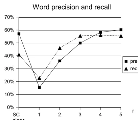
Concerning the detection of whole words, (fig-ure 2), the word precision is strictly increasing with r and ranges between 15.2% and 60.2%, the latter being a 3.2% increase with regard to the successor count alone. The word recall is lower when preprocessing is performed with
n = 1 (-18.2%), but higher in all other cases, with a peak of 56% for n= 4 (+15.2%).
Overall, we can say the segmentation
perfor-Figure 2: Word precision and recall ob-tained with the successor count alone and with utterance-boundary preprocessing on n-grams.
mance exhibited by our hybrid algorithm con-firms our expectations regarding the comple-mentarity of the two strategies examined: their combination is clearly superior to each of them taken independently. There may be a slight loss in precision, but it is massively counterbalanced by the gain in recall.
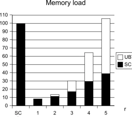
4.3 Memory load
The second hypothesis we made was that the preprocessing step would reduce the memory load of the successor count algorithm. In our implementation, the space used by each algo-rithm can be measured by the number of nodes of the trees storing the distributions. Five dis-tinct trees are involved: three for the utterance-boundary approach (one for the distribution of
n-grams in general and two for their distribu-tions in utterance-initial and -final position), and two for the predictability approach (one for successors and one for predecessors). The memory load of each algorithm is obtained by summation of these values.
As can be seen on figure 3, the size of the trees built by the successor count is drastically re-duced by preprocessing. Successor count alone uses as many as 99’405 nodes; after preprocess-ing, the figures range between 7’965 for n = 1 and 38’786 forn= 5 (SC, on the figure)8. How-ever, the additional space used by the n-grams
8
Figure 3: Memory load (in thousands of nodes) measured with the successor count alone and with utterance-boundary preprocessing on n -grams (see text).
distributions needed to compute the utterance-boundary typicality (UBT) grows quickly with
n, and the total number of nodes even exceeds that of the successor count alone when n = 5. Still, for lower values of n, preprocessing leads to a substantial reduction in total memory load.
4.4 Processing time
It seems unlikely that the combination of the two algorithms does not exhibit any drawback. We have said in section 3 that storing distribu-tions in a tree was not optimal from the point of view of time complexity, so we did not have high expectations on this topic. Nevertheless, we recorded the time used by the algorithms for the sake of completeness. CPU time9 was measured in seconds, using built-in functions of Perl, and the durations we report were averaged over 10 runs of the simulation10.
What can be seen on figure 4 is that although the time used by the successor count computa-tion is slightly reduced by preprocessing, this does not compensate for the additional time re-quired by the preprocessing itself. On average, the total time is multiplied by 1.6 when pre-processing is performed. Again, this is really a consequence of the chosen implementation, as this factor could be reduced to 1.15 by storing
9
on a pentium III 700MHz
10
This does not give a very accurate evaluation of pro-cessing time, and we plan to express it in terms of num-ber of computational steps.
Figure 4: Processing time (in seconds) mea-sured with the successor count alone and with utterance-boundary preprocessing on n-grams.
distributions in flat hash tables rather than tree structures.
5 Conclusions and discussion
In this paper, we have investigated two ap-proaches to speech segmentation based on dif-ferent heuristics: the utterance-boundary strat-egy, and the predictability strategy. On the ba-sis of former empirical results as well as theoret-ical considerations regarding their performance and complexity, we have suggested that the utterance-boundary approach could be used as a preprocessing step in order to lighten the task of the predictability approach without damag-ing the segmentation.
This intuition was translated into an explicit model, then implemented and evaluated for a task of word segmentation on a child-oriented phonetically transcribed french corpus. Our re-sults show that:
• the combined algorithm outperforms its component parts considered separately;
• the total memory load of the combined al-gorithm can be substantially reduced by the preprocessing step;
• however, the processing time of the com-bined algorithm is generally longer and possibly much longer depending on the im-plementation.
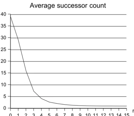
[image:6.604.73.286.84.272.2]Figure 5: Average successor count for n-grams (based on the corpus described in section 4.1).
computational morphology, Goldsmith (2001) uses Harris’ successor count as a means to re-duce the search space of a more powerful al-gorithm based on minimum description length (Marcken, 1996). We go one step further and show that an utterance-boundary heuristic can be used in order to reduce the complexity of the successor count algorithm11.
Besides complexity issues, there is a prob-lem ofdata sparsenesswith the successor count, as it decreases very quickly while the size n of the context grows. In the case of our quite re-dundant child-oriented corpus, the (weighted) average of the successor count12 for a random
n-gram Pw∈Snf(w)succ(w) gets lower than 1
for n ≥ 9 (see figure 5). This means that in most utterances, no more boundary can be in-serted after the first 9 phonemes (respectively before the last 9 phonemes) unless we get close enough to the other extremity of the utter-ance for the predecessor (respectively successor) count to operate. As regards the utterance-boundary typicality, on the other hand, the po-sition in the utterance makes no difference. As a consequence, many examples can be found in our corpus, where the middle part of a long ut-terance would be undersegmented by the succes-sor count alone, whereas preprocessing provides it with more tractable chunks. This is illus-trated by the following segmentations of the
ut-terance (Daddy doesn’t
11
at least as regards memory load, which could more restrictive in a developmental perspective
12
The predecessor count behaves much the same.
like carrots), where vertical bars denote bound-aries predicted by the utterance-boundary typ-icality (forr= 5), and dashes represent bound-aries inferred by the successor count:
SC !"
UBT (r = 5) #%$ !&$
UBT + SC '"$() !&$
This suggests that the utterance-boundary strategy could be more than an additional de-vice that safely predicts some boundaries that the successor count alone might have found or not: it could actually have a functional rela-tionship with it. If the predictability strategy has some relevance for speech segmentation in early infancy (Saffran et al., 1996), then it may be necessary to counterbalance the data sparse-ness; this is what these authors implicitely do by usingfirst-ordertransition probabilities, and it would be easy to define ann-th order succes-sor count in the same way. Yet another possi-bility would be to “reset” the successor count after each boundary inserted. Further research should bring computational and psychological evidence for or against such ways to address rep-resentativity issues.
We conclude this paper by raising an issue that was already discussed by Gammon (1969), and might well be tackled with our methodol-ogy. It seems that various segmentation strate-gies correlate more or less with different segmen-tation levels. We wonder if these different kinds of sensitivity could be used to make inferences about the hierarchical structure of utterances.
6 Acknowledgements
The author is grateful to Marianne Kilani-Schoch and the mother of Sophie for providing the acquisition corpus (see p.4), as well as to Fran¸cois Bavaud, Marianne Kilani-Schoch and two anonymous reviewers for useful comments on earlier versions of this paper.
References
R.N. Aslin, J.Z. Woodward, N.P. Lamendola, and T.G. Bever. 1996. Models of word seg-mentation in fluent maternal speech to in-fants. In J.L Morgan and Demuth K., ed-itors, Signal to Syntax: Bootstrapping from Speech to Grammar in Early Language Ac-quisition, pages 117–134. Lawrence Erlbaum Associates, Mahwah (NJ).
F. Bavaud and A. Xanthos. 2002. Thermody-namique et statistique textuelle: concepts et illustrations. In Actes des 6`e Journ´ees Inter-nationales d’Analyse Statistique des Donn´ees Textuelles (JADT 2002), pages 101–111. M.R. Brent and T.A. Cartwright. 1996.
Distri-butional regularity and phonotactics are use-ful for segmentation. Cognition, 61:93–125. M.H. Christiansen, J. Allen, and M. Seidenberg.
1998. Learning to segment speech using mul-tiple cues. Language and Cognitive Processes, 13:221–268.
A. Content, P. Mousty, and M. Radeau. 1990. Brulex: Une base de donn´ees lexicales in-formatis´ee pour le fran¸cais ´ecrit et parl´e. L’Ann´ee Psychologique, 90:551–566.
E. Gammon. 1969. Quantitative approxima-tions to the word. InPapers presented to the International Conference on Computational Linguistics COLING-69.
J. Goldsmith. 2001. Unsupervised learning of the morphology of a natural language. Com-putational Linguistics, 27 (2):153–198. Z.S. Harris. 1955. From phoneme to morpheme.
Language, 31:190–222.
J.L. Hutchens and M.D. Adler. 1998. Find-ing structure via compression. InProceedings of the International Conference on Computa-tional Natural Language Learning, pages 79– 82.
M. Kilani-Schoch and W.U. Dressler. 2001. Filler + infinitive and pre- and protomorphol-ogy demarcation in a french acquisition cor-pus. Journal of Psycholinguistic Research, 30 (6):653–685.
B. MacWhinney. 2000. The CHILDES Project: Tools for Analyzing Talk. Third Edition. Lawrence Erlbaum Associates, Mahwah (NJ). C.G. de Marcken. 1996. Unsupervised Language Acquisition. Phd dissertation, Massachusetts Institute of Technology.
J.R. Saffran, E.L. Newport, and R.N. Aslin. 1996. Word segmentation: The role of distri-butional cues. Journal of Memory and Lan-guage, 35:606–621.
A. Xanthos. 2003. Du k-gramme au mot: vari-ation sur un th`eme distributionnaliste. Bul-letin de linguistique et des sciences du langage (BIL), 21.