An efficient numerical algorithm for solving the two dimensional fractional cable equation

R E S E A R C H

Open Access

An efficient numerical algorithm for

solving the two-dimensional fractional cable

equation

Ming Zhu Li

_{, Li Juan Chen}

_{, Qiang Xu}

_{and Xiao Hua Ding}

*_{Correspondence:}

[email protected] 2_{School of Science, Qingdao}

University of Technology, Qingdao, China

Full list of author information is available at the end of the article

Abstract

In this paper, we consider an efficient numerical algorithm for solving the two-dimensional fractional cable equation. The stability and convergency of the numerical scheme are rigorously proved by the Fourier analysis. Then we find that the convergence order isO(

τ

x+h4y). Finally, numerical experiments are carried out to verify the accuracy and effectiveness of the new scheme.

Keywords: Fractional cable equation; Fourier analysis; Stability; Convergence

1 Introduction

Fractional differential equations have been studied by many researchers in recent years. The fact shows that fractional differential equations can describe many phenomena and processes in various fields of science and engineering [1–6]. Since the fractional operators are nonlocal and have the character of history dependence and universal mutuality, it is not easy even impossible to obtain the analytical solutions of fractional differential equations, especially in high-dimensional domains. Therefore, there has been a growing interest in developing numerical methods for fractional differential equations [7–17].

The cable equation is one of the most fundamental equations for modelling neuronal dynamics. A recent study [18] has found that the diffusion of molecules through the cy-toplasm of Purkinje cell dendrites is slowed at the macroscopic scale, primarily through temporary trapping by dendritic spines, and to a lesser extent through macromolecular crowding or binding [19,20]. Henry et al. [21] derived a fractional cable equation to model electrotonic properties of spiny neuronal dendrites, which is similar to the traditional ca-ble equation except that the order of derivative with respect to the space and/or time is fractional.

In this paper, we consider the following two-dimensional fractional cable equation:

∂u(x,y,t)

∂t =0D

1–γ1 t

κ1

∂2u(x,y,t)

∂x2 +κ2

∂2u(x,y,t)

∂y2

with the initial condition

u(x,y, 0) =ψ(x,y), 0≤x,y≤L, (2)

and the boundary conditions

u(0,y,t) =φ1(y,t), u(L,y,t) =φ2(y,t), 0≤y≤L, 0≤t≤T, (3)

u(x, 0,t) =ϕ1(x,t), u(x,L,t) =ϕ2(x,t), 0≤x≤L, 0≤t≤T, (4)

where 0 <γ1,γ2< 1, κ1, κ2 andκ3 are positive constants, andf(x,y,t),ψ(x,y),φ1(y,t),

φ2(y,t),ϕ1(x,t) andϕ2(x,t) are sufficiently smooth functions. The symbol0D1–γt u(x,y,t)

denotes the Riemann–Liouville fractional derivative of order 1 –γ with respect to vari-ablet, which is defined by

0D1–γt u(x,y,t) =

1

Γ(γ)

∂ ∂t

t

0

u(x,y,s)

(t–s)1–γ ds, 0 <γ < 1.

We mention some recent progress on the numerical treatment of the fractional cable equation. Liu et al. [22] presented two implicit numerical methods for the fractional ca-ble equation and discussed the stability and convergence of these methods using the en-ergy method. Lin et al. [23] constructed a finite difference/Legendre spectral scheme for the fractional cable equation. Hu et al. [24] proposed two implicit compact difference schemes for the fractional cable equation and analyzed the stability and convergence of the first scheme. Zheng et al. [25] used the discontinuous Galerkin finite element to approx-imate the fractional cable equation. Zhang et al. [26] presented discrete-time orthogonal spline collocation methods for the two-dimensional fractional cable equation. Irandoust-Pakchin et al. [27] employed the method of Chebyshev cardinal functions for solving the variable-order nonlinear fractional cable equation. Dehghan et al. [28] applied the ele-ment free Galerkin (EFG) method for solving fractional cable equation with the Dirich-let boundary condition. Zhu er al. [29] proposed two fully discrete schemes, based on Galerkin finite element schemes and the convolution quadrature method. Yu et al. [30] provided a fourth-order compact finite difference method for two-dimensional fractional cable equation. Liu et al. [31,32] presented the finite element method for the nonlinear time-fractional cable equation. However, to the best of our knowledge, there is no nu-merical scheme with second-order accuracy in time for the two-dimensional fractional equation. Our scheme in this paper can reach to second-order accuracy in time. We inte-grate both sides of the fractional cable equation with respect to the timet, and then use the Riemann–Liouville fractional integral definition to discretize the fractional term.

It follows from the Lagrange interpolation formula that

Using a Taylor expansion, we have

and

Similarly, we obtain the following approximation forI2andI3:

I2=μ2

where

Rk_i,j=R11+R12+R13+O

τ3

=Oτ2+h4_x+h4_y

_k

n=1

tn

tn–1

(tk–s)γ1–1ds– k–1

n=1

tn

tn–1

(tk–1–s)γ1–1ds

+Oτ2

_k

n=1

tn

tn–1

(tk–s)γ2–1ds– k–1

n=1

tn

tn–1

(tk–1–s)γ2–1ds

+Oτ3.

Since

k

n=1

tn

tn–1

(tk–s)γ–1ds– k–1

n=1

tn

tn–1

(tk–1–s)γ–1ds=

1

γ

(kτ)γ– (kτ–τ)γ,

forkτ≤T,

Rk_i,j=Oτ2+h4_x+h4_y. (19)

Omitting the small termRk

i,jand replacing the functionuki,jwith its numerical

approxi-mationU_ik_,jin (18), we can get the following difference scheme for (1):

HxHyUik,j–HxHyUik,j–1

=μ1

k

n=0

a(γ1) n –b(γn1)

Hyδ2xUik,j–n+μ2

k

n=0

a(γ1) n –b(γn1)

Hxδ2yUik,j–n

–μ3

k

n=0

a(γ2) n –b(γn2)

HxHyUik,j–n+ τ

2HxHy

f_ik_,j+f_ik_,j–1. (20)

In addition, the initial and boundary value conditions can be written as

U_i0_,j=ψ(ihx,jhy), i= 0, 1, . . . ,M1,j= 0, 1, . . . ,M2,

U_0,k_j=φ1(jhy,kτ), UMk1,j=φ2(jhy,kτ), j= 0, 1, . . . ,M2,k= 1, 2, . . . ,N,

U_ik_,0=ϕ1(ihx,kτ), Uik,M2=ϕ2(ihx,kτ), i= 0, 1, . . . ,M1,k= 1, 2, . . . ,N.

(21)

3 Stability analysis

In this section, we will analyze the stability of the scheme (20) by using the Fourier analysis. LetU_ijkbe the approximate solution of (20) and define

ρ_ik_,j=U_ik_,j–U_ik_,j, i= 0, 1, . . . ,M1– 1,j= 0, 1, . . . ,M2– 1,k= 0, 1, . . . ,N, (22)

and

ρk=ρ₁₁k,ρ₁₂k, . . . ,ρ_1,k_M2–1,ρk₂₁,ρ₂₂k, . . . ,ρ_2,k_M2–1, . . . ,ρ_Mk_1–1,1,

ρ_Mk

1–1,2, . . . ,ρ k M1–1,M2–1

With the above definition and regarding to (20), we can easily get the following roundoff error equation:

HxHyρki,j–HxHyρik,j–1

=μ1

k

n=0

a(γ1) n –b(γn1)

Hyδ2xρik,j–n+μ2

k

n=0

a(γ1) n –b(γn1)

Hxδ2yρik,j–n

–μ3

k

n=0

a(γ2)

n –b(γn2)

HxHyρik,j–n. (24)

Fork= 0, 1, . . . ,N, define the grid function

ρk(x,y) =

⎧ ⎪ ⎪ ⎪ ⎪ ⎪ ⎨ ⎪ ⎪ ⎪ ⎪ ⎪ ⎩

ρ_ik_,j, xi–

hx

2 <x≤xi+

hx

2, i= 1, 2, . . . ,M1– 1, yj–h₂y <y≤yj+h₂y, j= 1, 2, . . . ,M2– 1,

0, 0≤x≤

hx

2 or L–

hx

2 <x≤L,

0≤y≤h₂y or L–h₂y<y≤L,

whereρk_{(x,y) can be expanded in a Fourier series}

ρk(x,y) =

∞

l1=–∞

∞

l2=–∞

ξk(l1,l2)eq2π(l1x/L+l2y/L), k= 1, 2, . . . ,N, (25)

in which

q=√–1, ξk(l1,l2) =

1

L2

L

0

L

0

ρk(x,y)e–q2π(l1x/L+l2y/L)_{dx dy.}

We introduce the following norm [33]:

ρk₂=

L

0

ρk(x,y)2dx dy

1 2

.

Using the Parseval equality, we have

ρk₂=

_∞

l1=–∞

∞

l2=–∞

ξk(l1,l2) 2

1 2

. (26)

According to the above analysis, we suppose that the solution of Eq. (24) has the follow-ing form:

ρ_ik_,j=ξkeqσ1ihx+qσ2jhy, (27)

Theorem 1 Suppose thatξk(k= 1, 2, . . . ,N)are the solution of(28),under the conditions

of Lemma2,we have

|ξk| ≤ |ξ0|, k= 1, 2, . . . ,N. (32)

Proof We prove (32) by means of mathematical induction. Fork= 1 from (28), we can write

From Lemmas1and2, the above equation leads to

|ξ1|= ω1– (a

Now we suppose that

+ μ3ω1

which completes the proof.

Theorem 2 Under the conditions of Lemma2,the compact difference scheme(20)is stable.

Proof From (26) and (32) we can write

which means that the proposed scheme is stable.

4 Convergence analysis

In this section, we discuss the convergence of the difference scheme (20). Similar to the stability analysis, we define the grid functions as follows:

We introduce the following norm [33]:

ek₂=

L

0

L

0

ζk(x,y)2dx dy

1 2

, (38)

Rk₂=

L

0

L

0

ηk(x,y)2dx dy

1 2

, (39)

where

ek=ek₁₁,ek₁₂, . . . ,e_1,k_M2–1,ek₂₁,ek₂₂, . . . ,ek_2,M2–1, . . . ,ek_M1–1,1,e_Mk_1–1,2, . . . ,ek_{M1–1,M2–1},

Rk=Rk₁₁,Rk₁₂, . . . ,R_1,k_M2–1,Rk₂₁,Rk₂₂, . . . ,Rk_2,M2–1, . . . ,Rk_M1–1,1,R_Mk_1–1,2, . . . ,Rk_{M1–1,M2–1}. Applying the Parseval equality, we have

ek2=

_∞

l1=–∞

∞

l2=–∞

ζk(l1,l2)2

1 2

, (40)

Rk2=

_∞

l1=–∞

∞

l2=–∞

ηk(l1,l2) 2

1 2

. (41)

From (19) there is a positive constantC0such that

Rk_i,j≤C0

τ2+h4_x+h4_y. (42)

Subtracting (20) from (18), we can obtain the following error equation:

HxHyeki,j–HxHyeki,–1j

=μ1

k

n=0

a(γ1) n –b(γn1)

Hyδ2xeki,–jn+μ2

k

n=0

a(γ1) n –b(γn1)

Hxδ2yeki,–jn

–μ3

k

l=0

a(γ2) n –b(γn2)

HxHyeik,–jn+Rki,j,

i= 0, 1, . . . ,M1– 1,j= 0, 1, . . . ,M2– 1,k= 0, 1, . . . ,N, (43)

and

e0_i,j= 0, 0≤i≤M1, 0≤j≤M2,

ek_0,j=ek_M1,j= 0, 0≤j≤M2, 0≤k≤N, (44) ek_i,0=ek_i,M2= 0, 0≤i≤M1, 0≤k≤N,

whereek

ij=ukij–Uijk.

According to the above analysis, we suppose that the solution of Eq. (43) has the follow-ing forms:

Substituting the above relations into (43), we obtain

ζk=

ω1– (a(γ11)–b (γ1)

1 )μ1ω2– (a(γ11)–b (γ1)

1 )μ2ω3– (a(γ12)–b (γ2)

1 )μ3ω1

ω1+μ1ω2+μ2ω3+μ3ω1

ζk–1

+ μ1ω2+μ2ω3

ω1+μ1ω2+μ2ω3+μ3ω1

k

n=2

a(γ1) n –b(γn1)

ζk–n

+ μ3ω1

ω1+μ1ω2+μ2ω3+μ3ω1

k

n=2

a(γ2)

n –b(γn2)

ζk–n

+ 1

ω1+μ1ω2+μ2ω3+μ3ω1

ηk. (46)

Noting thate0_{= 0, we have}

ζ0=ζ0(l1,l2) = 0.

Due to the convergence of the series in the right hand side of (41), there is a positive con-stantC1such that

|ηk| ≡ηk(l1,l2)≤C1τη1(l1,l2)≡C1τ|η1|, k= 1, 2, . . . ,N. (47)

Theorem 3 Ifζk(k= 1, 2, . . . ,N)be the solutions of(46),under the conditions of Lemma2,

we have

|ζk| ≤k

9

4C1τ|η1|, k= 1, 2, . . . ,N.

Proof Fork= 1 in (46), we have

|ζ1|= 1

ω1+μ1ω2+μ2ω3+μ3ω1|

η1| ≤9

4C1τ|η1|. Now we suppose that

|ζn| ≤n

9

4C1τ|η1| (n= 1, 2, . . . ,k– 1). (48) From (46) and (48), we have

|ζk| ≤

ω1– (a(γ11)–b (γ1)

1 )μ1ω2– (a(γ11)–b (γ1)

1 )μ2ω3– (a(γ12)–b (γ2)

1 )μ3ω1

ω1+μ1ω2+μ2ω3+μ3ω1

|ζk–1|

+ μ1ω2+μ2ω3

ω1+μ1ω2+μ2ω3+μ3ω1

k

n=2

_a(γ1)

n –b(γn1)|ζk–n|

+ μ3ω1

ω1+μ1ω2+μ2ω3+μ3ω1

k

n=2

a(γ2)

+ 1

From the above discussion, the conditions of Lemma2are sufficient. However, numer-ical simulations for a wide range ofγ1 andγ2 in the next section demonstrate that the

stability and convergence of the scheme are generally established.

5 Numerical experiments

In this section, some numerical results are given to testify the effectiveness and conver-gence orders of our new proposed scheme. To illustrate the accuracy of the method and for the comparison, we take the same spatial stephx=hy=h, and denote theL2andL∞

norm errors of the numerical solution as follows:

e2(h,τ) = max 0≤n≤N

Un–un,

e∞(h,τ) = max

0≤n≤N

Un–un_∞.

Furthermore, the temporal convergence order and the spatial convergence order are de-fined by

rate1 =log₂

e2(h, 2τ) e2(h,τ)

,

rate2 =log₂

e∞(h, 2τ)

e∞(h,τ)

,

whenhis sufficiently small, and

rate3 =log₂

e2(2h,τ) e2(h,τ)

,

rate4 =log₂

e∞(2h,τ)

e∞(h,τ)

,

whenτ is sufficiently small, respectively.

Example1 Consider the following two-dimensional fractional cable equation:

∂u(x,y,t)

∂t =0D

1–γ1 t

∂2u(x,y,t)

∂x2 +

∂2u(x,y,t)

∂y2

–0D1–γt 2u(x,y,t) +f(x,y,t),

0 <x,y< 1, 0 <t≤1, (50) with the initial condition

u(x,y, 0) = 0, 0≤x≤1, and the boundary conditions

u(0,y,t) = 0, 0≤t≤1,

u(1,y,t) = 0, 0≤t≤1,

u(x, 0,t) = 0, 0≤t≤1,

where

f(x,y,t) =

2t+ 2

Γ(2 +γ1)

t1+γ1₊ 4π

2

Γ(2 +γ2) t1+γ2

sin(πx)sin(πy).

The exact solution of Eq. (50) isu(x,t) =t2_{sin(πx)sin(πy).}

We use the difference scheme (20) to solve the above equation. Firstly, the temporal errors and convergence orders are given in Table1. We take the sufficiently small spatial steph= 1

128 and variousγ1andγ2, respectively. It is observed that the scheme generates

temporal convergence order, which is consistent with our theoretical analysis. Secondly, the spatial errors and convergence orders are tabulated in Table2. We take the sufficiently small temporal stepτ=₂₀₀₀1 and variousγ1andγ2, respectively. The results illustrate that

our scheme has accuracy ofO(h4_{) in the spatial direction. That is in good agreement with}

our theoretical analysis.

Table 1 Numerical errors and convergence orders in time direction withh=₁₂₈1

τ e2(h,τ) rate1 e_∞(h,τ) rate2

γ1= 0.9,γ2= 0.8 1/20 3.1063e-4 ∗ 6.2126e-4 ∗

1/40 7.7663e-5 1.9999 1.5532e-4 1.9998

1/80 1.9416e-5 2.0000 3.8832e-5 1.9999

1/160 4.8537e-6 2.0001 9.7074e-6 2.0001

γ1= 0.8,γ2= 0.6 1/20 3.0836e-4 ∗ 6.1672e-4 ∗

1/40 7.7136e-5 1.9991 1.5427e-4 1.9991

1/80 1.9291e-5 1.9995 3.8582e-5 1.9995

1/160 4.8233e-6 1.9998 9.6467e-6 1.9998

γ1= 0.6,γ2= 0.2 1/20 2.9879e-4 ∗ 5.9758e-4 ∗

1/40 7.5111e-5 1.9920 1.5022e-4 1.9920

1/80 1.8851e-5 1.9944 3.7702e-5 1.9944

1/160 4.7253e-6 1.9961 9.4507e-6 1.9965

γ1= 0.2,γ2= 0.6 1/20 2.1680e-4 ∗ 4.3360e-4 ∗

1/40 5.6905e-5 1.9297 1.1381e-4 1.9297

1/80 1.4814e-5 1.9415 2.9629e-5 1.9415

1/160 3.8312e-6 1.9511 7.6624e-6 1.9511

Table 2 Numerical errors and convergence orders in spatial direction withτ=₂₀₀₀1

hx=hy e2(h,τ) rate3 e∞(h,τ) rate4

γ1= 0.9,γ2= 0.8 1/4 7.0259e-4 ∗ 1.4052e-3 ∗

1/8 4.3084e-5 4.0274 8.6167e-5 4.0275

1/16 2.6514e-6 4.0223 5.3027e-6 4.0223

1/32 1.3649e-7 4.2798 2.7299e-7 4.2798

γ1= 0.8,γ2= 0.6 1/4 7.0294e-4 ∗ 1.4059e-3 ∗

1/8 4.3105e-5 4.0275 8.6210e-5 4.0274

1/16 2.6527e-6 4.0223 5.3054e-6 4.0223

1/32 1.3656e-7 4.2799 2.7312e-7 4.2798

γ1= 0.6,γ2= 0.2 1/4 7.0338e-4 ∗ 1.4067e-3 ∗

1/8 4.3132e-5 4.0274 8.6265e-5 4.0274

1/16 2.6547e-6 4.0221 5.3095e-6 4.0221

1/32 1.3705e-7 4.2757 2.7411e-7 4.2757

γ1= 0.2,γ2= 0.6 1/4 7.4232e-4 ∗ 1.4846e-3 ∗

1/8 4.5522e-5 4.0274 9.1044e-5 4.0274

1/16 2.8069e-6 4.0195 5.6139e-6 4.0194

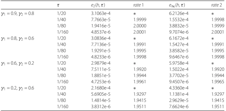
Figure 1Numerical and exact solutions with

γ1= 0.3,γ2= 0.5,hx=hy=641 andτ= 1 512att= 1

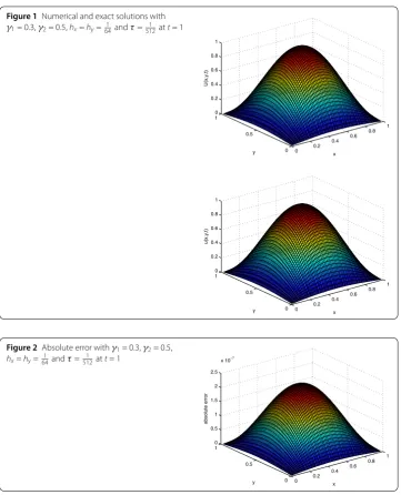
Figure 2Absolute error withγ1= 0.3,γ2= 0.5,

hx=hy=₆₄1 andτ=₅₁₂1 att= 1

Figures1and2present the graphs of the numerical solution, the exact solution and the absolute error withγ1= 0.3,γ2= 0.5,hx=hy= ₆₄1 andτ =₅₁₂1 . From these diagrams, it

can be seen that our scheme gives a good approximation to the exact solution at mesh points.

The comparisons of our numerical solutions and the results of method developed in [26] for variousγ1andγ2are shown in Table3. It can be seen that the accuracy of our scheme

is superior to the scheme proposed in [26] .

6 Conclusion

Table 3 Comparison of errors between the scheme (20) and the scheme given in [26]

hx=hy=τ e2(h,τ) e∞(h,τ) e2(h,τ) [26] e∞(h,τ) [26]

γ1= 0.9,γ2= 0.4 1/5 4.8507e-3 9.7013e-3 2.7115e-2 5.3825e-2

1/10 1.2286e-3 2.4074e-3 1.0684e-2 2.1395e-2

1/20 3.0928e-4 6.1511e-4 4.1439e-3 8.2895e-3

1/30 1.3769e-4 2.7467e-4 2.3706e-3 4.7416e-3

γ1= 0.6,γ2= 0.8 1/5 4.6336e-3 9.2673e-3 5.0394e-3 9.7966e-3

1/10 1.1881e-3 2.3281e-3 1.6070e-3 3.2412e-3

1/20 3.0103e-4 5.9869e-4 5.0187e-4 1.0054e-3

1/30 1.3436e-4 2.6804e-4 2.5264e-4 5.0562e-4

γ1= 0.5,γ2= 0.5 1/5 4.4248e-3 8.8496e-3 1.9661e-2 3.8921e-2

1/10 1.1486e-3 2.2508e-3 7.2986e-3 1.4625e-2

1/20 2.9324e-4 5.8320e-4 2.6612e-3 5.3241e-3

1/30 1.3133e-4 2.6199e-4 1.4673e-3 2.9349e-3

Acknowledgements

The authors are very grateful for the editors and the referees carefully reading and comments on this paper.

Funding

The research supported by the Natural Science Foundation of Shandong Province under grant No. ZR2017BA007.

Competing interests

The authors declare that they have no competing interests.

Authors’ contributions

All authors contributed equally to the writing of this paper. All authors read and approved to the final manuscript.

Author details

1_{Department of Mathematics, Harbin Institute of Technology, Harbin, China.}2_{School of Science, Qingdao University of}

Technology, Qingdao, China. 3_{School of Mathematics and Statistics, Shandong Normal University, Jinan, China.}

Publisher’s Note

Springer Nature remains neutral with regard to jurisdictional claims in published maps and institutional affiliations.

Received: 7 June 2018 Accepted: 9 November 2018 References

1. Podlubny, I.: Fractional Differential Equations. Academic Press, New York (1999)

2. Raberto, M., Scalas, E., Mainardi, F.: Waiting-times and returns in high-frequency financial data: an empirical study. Physica A314, 749–755 (2002)

3. Koeller, R.C.: Application of fractional calculus to the theory of viscoelasticity. J. Appl. Mech.51, 229–307 (1984) 4. Meerschaert, M.M., Zhang, Y., Baeumerc, B.: Particle tracking for fractional diffusion with two time scales. Comput.

Math. Appl.59, 1078–1086 (2010)

5. Jiang, X., Xu, M., Qi, H.: The fractional diffusion model with an absorption term and modified Fick’s law for non-local transport processes. Nonlinear Anal.11, 262–269 (2011)

6. Wang, Z., Wang, X., Li, Y., Huang, X.: Stability and Hopf bifurcation of fractional-order complex-valued single neuron model with time delay. Int. J. Bifurc. Chaos27(13), 1750209 (2017)

7. Zayernouri, M., Karniadakis, G.E.: Fractional spectral collocation methods for linear and nonlinear variable order FPDEs. J. Comput. Phys.293, 312–338 (2015)

8. Mohebbi, A., Abbaszadeh, M.: Compact finite difference scheme for the solution of time fractional advection-dispersion equation. Numer. Algorithms63, 431–452 (2013)

9. Sousa, E., Li, C.: A weighted finite difference method for the fractional diffusion equation based on the Riemann–Liouville derivative. Appl. Numer. Math.90, 22–37 (2015)

10. Guo, B.L., Xu, Q., Yin, Z.: Implicit finite difference method for fractional percolation equation with Dirichlet and fractional boundary conditions. Appl. Math. Mech.37, 403–416 (2016)

11. Jin, B., Lazarov, R., Pasciak, J., Zhou, Z.: Error analysis of semidiscrete finite element methods for inhomogeneous time-fractional diffusion. Appl. Numer. Math.90, 22–37 (2015)

12. Bhrawy, A.H., Doha, E.H., Baleanud, D., Ezz-Eldien, S.S.: A spectral tau algorithm based on Jacobi operational matrix for numerical solution of time fractional diffusion-wave equations. J. Comput. Phys.93, 142–156 (2015)

13. Srivastava, P.K., Kumar, M., Mohapatra, R.N.: Numerical simulation with high order accuracy for the time fractional reaction subdiffusion equation. Comput. Math. Appl.62, 1707–1714 (2011)

14. Li, X.H., Wong, P.J.Y.: A higher order non-polynomial spline method for fractional sub-difffusion problems. J. Comput. Phys.328, 46–65 (2017)

15. Hicdurmaz, B., Ashyralyev, A.: A stable numerical method for multidimensional time fractional Schrödinger equations. Comput. Math. Appl.72, 1703–1713 (2016)

17. Wang, Z.: A numerical method for delayed fractional-order differential equations. J. Appl. Math.2013, 256071 (2013) 18. Santamaria, F., Wils, S., Schutter, E.D., Augustine, G.J.: Anomalous diffusion in Purkinje cell dendrites caused by spines.

Neuron52, 635–648 (2006)

19. Schnell, S., Turner, T.E.: Reaction kinetics in intracellular environments with macromolecular crowding: simulations andratelaws. Prog. Biophys. Mol. Biol.85, 235–260 (2004)

20. Weiss, M., Elsner, M., Kartberg, F., Nilsson, T.: Anomalous subdiffusion is a measure for cytoplasmic crowding in living cells. Biophys. J.87, 3518–3524 (2004)

21. Henry, B.I., Langlands, T.A., Wearne, S.L.: Fractional cable models for spiny neuronal dendrites. Phys. Rev. Lett.100, 128103 (2008)

22. Liu, F., Yang, Q., Turner, I.: Two new implicit numerical methods for the fractional cable equation. J. Comput. Nonlinear Dyn.6, 011009 (2011)

23. Lin, Y., Li, X., Xu, C.: Finite difference spectral approximations for the fractional cable equation. Math. Comput.80, 1369–1396 (2009)

24. Hu, X., Zhang, L.: Implicit compact difference schemes for the fractional cable equation. Appl. Math. Model.36, 4027–4043 (2012)

25. Zheng, Y., Zhao, Z.: The discontinuous Galerkin finite element method for fractional cable equation. Appl. Numer. Math.115, 32–41 (2017)

26. Zhang, H., Yang, X., Han, X.: Discrete-time orthogonal spline collocation method with application to two-dimensional fractional cable equation. Comput. Math. Appl.68, 1710–1722 (2014)

27. Irandoust-Pakchin, S., Abdi-Mazraeh, S., Khani, A.: Numerical solution for a variable-order fractional nonlinear cable equation via Chebyshev cardinal functions. Comput. Math. Math. Phys.236, 209–224 (2011)

28. Dehghan, M., Abbaszadeh, M.: Analysis of the element free Galerkin (EFG) method for solving fractional cable equation with Dirichlet boundary condition. Appl. Numer. Math.109, 208–234 (2016)

29. Zhu, P., Xie, S., Wang, X.: Nonsmooth data error estimates for FEM approximations of the time fractional cable equation. Appl. Numer. Math.121, 170–184 (2017)

30. Yu, B., Jiang, X.: Numerical identification of the fractional derivatives in the two-dimensional fractional cable equation. J. Sci. Comput.68, 252–272 (2016)

31. Liu, Y., Du, Y.W., Li, H., Wang, J.F.: A two-grid finite element approximation for a nonlinear time-fractional cable equation. Nonlinear Dyn.85(4), 2535–2548 (2016)

32. Liu, Y., Du, Y.W., Li, H., Liu, F., Wang, J.F.: Some second-orderθschemes combined with finite element method for nonlinear fractional cable equation. Numer. Algorithms (2018).https://doi.org/10.1007/s11075-018-0496-0 33. Chen, S., Liu, F., Zhuang, P., Anh, V.: Finite difference approximations for the fractional Fokker–Planck equation. Appl.