R E S E A R C H
Open Access
Triangular integrals for 2-, 3- and 4-variable
functions
Kiyohisa Tokunaga
**Correspondence:
kiyohisa@bene.fit.ac.jp
Laboratory of Information Science, Fukuoka Institute of Technology, Wajiro, Higashi-ku, Fukuoka, 811-0295, Japan
Abstract
The triangular integrals for 2-, 3- and 4-variable functions are respectively and precisely defined as the single limits of double, triple, and quadruple sums in detail. A corollary of the divergence theorem in each dimension is useful to determine the triangular integral value. The indices of the sequence of the integrand must coincide with those of the corresponding integral variable to calculate the correct triangular integral value. In a triangular triple integral, one kind of two sets of increments is inappropriate for the convergence of numerical values, but the other kind is able to calculate numerical values by a computer algebra system.
1 Introduction
The primary theme of this article is a double integral for a -variable functionp=p(x,y) in a domainDon the D plane. A double integral is usually regarded as a rectangular double integral. The calculation process of the rectangular double integral [, ] is con-ventionally defined as the double limits at infinity of double independent sums,n→ ∞
fori= , , . . . ,nandk→ ∞forj= , , . . . ,k, of rectangularly divided areas by
D
p(x,y)dx dy= lim
n→∞ n
i= lim k→∞
k
j=
p(xi,yj)xiyj, (.)
wherexi=xi–xi–andyj=yj–yj–. On the other hand, atriangle meshor
triangu-lar meshis widely used in the computer graphics. In addition to introducing triangular
elements in the finite element method [], a combination of a triangular area method and double dependent series was applied to sweep all of the area []. Proenca¸ and Filipe showed the advantage of a triangular region in comparison with rectangular one for a finite area in real-time face detection. They only investigated a finite sum of finite triangular areas, but our theory of the triangular integral [, ] treats infinite sum of infinitesimal trian-gular areas. Moreover, it involves the total differential and the antisymmetric property []. The calculation process of the triangular double integral on the D plane, where tri-angular double integral is expressed as (.), has not been defined even in the previous article []. A corollary of the divergence theorem on the D plane is useful to determine the triangular double integral value. The indices of the sequence of the integrand must co-incide with those of the corresponding integral variable to calculate the correct triangular integral value. The calculation process of the triangular double integral for a -variable function on the D plane is precisely defined as the single limit of double dependent sums
by (.) in Definition . Applying Definition , it is able to calculate numerical values by a computer algebra system in Example .
The secondary theme of this article is a triple integral for a -variable functionq=
q(x,y,z) in a domain Din the D space. A triple integral is usually regarded as a rect-angular triple integral. The calculation process of the rectrect-angular triple integral is con-ventionally defined as the triple limits at infinities of triple independent sums,n→ ∞for
i= , , . . . ,nandk→ ∞forj= , , . . . ,kandm→ ∞forl= , , . . . ,m, of rectangularly divided volumes by
D
q(x,y,z)dx dy dz= lim
n→∞ n
i= lim k→∞
k
j= lim m→∞
m
l=
q(xi,yj,zl)xiyjzl, (.)
wherexi=xi–xi–,yj=yj–yj–, andzl=zl–zl–. As shown in the previous article [], a triangular triple integral can be expressed as (.). A corollary of the divergence theorem in the D space is useful to determine the triangular triple integral value. In this calculation process of the triangular triple integral, new difficulty has arisen. For the inte-grand of the divergence theorem in the D space, there two alternative ways of decompo-sition of two kinds of double sequences (Xμ)
j,kand (Xμ)k,jforμ= , , andj= , , . . . ,k andk= , , . . . ,n. One way is used in the previous article [], the other way is used as (.) and (.) in this article. One kind of the two sets of increments{i(xγ)i,,h(xγ)j,h}and
{i(xγ),i,h(xγ)h,j}forγ= , , andi= , , . . . ,jandj,h= , , . . . ,kused in the previous article [] is inappropriate for convergence of integral values since it is unable to calculate numerical values by a computer algebra system in Example . However, the other kind of two sets of increments
. {h(xγ),h,i(xγ)i,k}, derived from (.),
. {h(xγ)h,,i(xγ)k,i}, derived from (.)
forγ = , , andi= , , . . . ,jandh= , , . . . ,kandk= , , . . . ,nused in this article is able to calculate numerical values by a computer algebra system in Example . We formulate the divergence theorem in the D space and related corollary based on the appropriate two sets of increments in this article. The calculation process of the triangular triple integral for a -variable function in the D space is precisely defined as the single limit of triple dependent sums by (.) in Definition .
The tertiary theme of this article is quadruple integral for a -variable function w=
w(t,x,y,z) in a domainDin the D time-space. Quadruple integral is usually regarded as the rectangular quadruple integral. The calculation process of the rectangular quadru-ple integral is conventionally defined as the quadruquadru-ple limits at infinities of quadruquadru-ple independent sums,s→ ∞forh= , , . . . ,sandn→ ∞fori= , , . . . ,nandk→ ∞for
j= , , . . . ,kandm→ ∞forl= , , . . . ,m, of rectangularly divided hyper-volumes by
D
w(t,x,y,z)dt dx dy dz
= lim s→∞
s
h= lim n→∞
n
i= lim k→∞
k
j= lim m→∞
m
l=
w(th,xi,yj,zl)th,xiyjzl, (.)
the D time-space is useful to determine the triangular quadruple integral value. Incre-ments in the D time-space are replaced for the convergence of the triangular integral value. One kind of six sets of increments{m(xδ),,m,i(xδ)i,,l,h(xδ)j,h,l},{m(xδ),m,,
i(xδ)i,l,,h(xδ)j,l,h},{m(xδ)m,,,i(xδ)l,i,,h(xδ)l,j,h},{m(xδ)m,,,i(xδ)l,,i,h(xδ)l,h,j},
{m(xδ),m,,i(xδ),l,i,h(xδ)h,l,j} and {m(xδ),,m,i(xδ),i,l,h(xδ)h,j,l} for δ = , , , and m= , , . . . ,l and i,l = , , . . . ,j and j,h = , , . . . ,k used in the previous arti-cle [] is inappropriate since they are the extension of the inappropriate increments
{i(xγ)i,,h(xγ)j,h} and {i(xγ),i,h(xγ)h,j} for γ = , , and i= , , . . . ,j and j,h= , , . . . ,k to in the D time-space. For the integrand of the divergence theorem in the D time-space, there are six alternative ways of decomposition of six kinds of triple sequences (Xμ)
j,k,l, (Xμ)j,l,k, (Xμ)l,j,k, (Xμ)l,k,j, (Xμ)k,l,j, and (Xμ)k,j,l forμ= , , , and
l= , , . . . ,jandj= , , . . . ,kandk= , , . . . ,n. Extending the appropriate set of the in-crements{h(xγ),h,i(xγ)i,k}and{h(xγ)h,,i(xγ)k,i}forγ = , , andi= , , . . . ,jand
j,h= , , . . . ,kandk= , , . . . ,nin the D space to in the D time-space, another kind of six sets of increments
. {h(xδ),h,,i(xδ)i,k,,m(xδ)j,k,m}, derived from (.),
. {h(xδ),,h,i(xδ)i,,k,m(xδ)j,m,k}, derived from (.),
. {h(xδ),,h,i(xδ),i,k,m(xδ)m,j,k}, derived from (.),
. {h(xδ),h,,i(xδ),k,i,m(xδ)m,k,j}, derived from (.),
. {h(xδ)h,,,i(xδ)k,,i,m(xδ)k,m,j}, derived from (.),
. {h(xδ)h,,,i(xδ)k,i,,m(xδ)k,j,m}, derived from (.)
forδ= , , , andm= , , . . . ,landi= , , . . . ,jandh,j= , , . . . ,k andk= , , . . . ,n
is derived in this article. This kind of six sets of increments is used in Definition . We formulate the divergence theorem in the D time-space and related corollary based on the appropriate sets of increments in this article. The calculation process of the triangular quadruple integral for a -variable function in the D time-space is precisely defined as the single limit of quadruple dependent sums by (.) in Definition .
This article is basically about the calculation processes of the triangular double, triple and quadruple integrals for -, - and -variable functions. This article also includes re-visions of the divergence theorems and the related corollaries based on the appropriate increments of the double and the triple sequences in the calculation processes of the tri-angular triple and quadruple integrals for - and -variable functions.
This article is structured as follows. In Section , the divergence theorem of the triangu-lar integral and a related coroltriangu-lary on the D plane are reviewed. The calculation process of the triangular double integral for a -variable function is precisely defined in detail. In Section , the divergence theorem of the triangular integral and a related corollary in the D space are revised based on the appropriate increments of the double sequence. The calculation process of the triangular triple integral for a -variable function is precisely defined in detail. In Section , the divergence theorem of the triangular integral and a related corollary in the D time-space are revised based on the appropriate increments of the triple sequence. The calculation process of the triangular quadruple integral for a -variable function is precisely defined in detail.
2 Triangular double integral on the 2D plane
in Section .. Component representation and an example of it for a -variable function are shown in Section .. In the following, the Cartesian coordinates are denotedx=x andx=y.
2.1 One kind of finite line element vector on the 2D plane
For triangular double integral, the following increments of single sequence of points on the D plane are introduced.
The increments of single sequence of points (xα)
kare denoted as follows:
xαk≡xαk–xαk– (.)
forα= , andk= , , . . . ,n.
The finite line element vector(lα)
kforα= , andk= , , . . . ,nis introduced as
lαk= –xαk. (.)
The antisymmetric symbol on the D plane is
εαβ=εαβ= ⎧ ⎪ ⎪ ⎨ ⎪ ⎪ ⎩
+ forε=ε,
– forε=ε , otherwise.
(.)
Using the antisymmetric symbol in (.), the antisymmetric finite line element vector (lμ)kforμ= , andk= , , . . . ,nis introduced as
(lμ)k=εαμ
lα
k (.)
and expressed as
(lμ)k= –εαμ
xαk, (.)
where the index is summed overα= , .
For example, we consider the case that the boundary of the domain is an ellipse:
x
a+
y
b = , (.)
wherea> andb> . The following is shown inThe curl theorem of a triangular
inte-gral[].
The Cartesian coordinates of the sequence of points (xj,yj) forj= , , , . . . ,k, and (xk,yk) fork= , , , . . . ,non the ellipse (.) are respectively expressed as
xj=acosϕj, yj=bsinϕj, (.)
where angular arithmetic sequencesϕjandϕkare respectively
ϕj=
j
nπ, (.)
ϕk=
k
nπ. (.)
2.2 Triangular double integral for a 2-variable function
Assume thatDis a domain and∂Dis the boundary of the domain on the D plane, ex-pressed in the Cartesian coordinates (x,y)∈R. LetX=X=X(x,y) andX=Y=Y(x,y) be partially differentiable functions with respect tox=xandx=yinD. There is only ! = kind of single sequence
Xμ
k= (Xk,Yk) (.)
forμ= , andk= , , , . . . ,n. There are ! = sets of possible partial increments for a -variable function.
The total increments of (Xμ)
jforμ= , andj= , , . . . ,kare denoted
Xμj≡Xμj–Xμj–
=Xμ(x
j,yj) –Xμ(xj–,yj–). (.)
The increments of (xβ)
jforβ= , andj= , , . . . ,kare denoted
xβj≡xβj–xβj–. (.)
The sets of possible partial increments of (Xμ)
jforμ= , andj= , , . . . ,kare denoted
Xμ[xj] =Xμ(xj,yj) –Xμ(xj–,yj), (.)
Xμ[yj] =Xμ(xj–,yj) –Xμ(xj–,yj–). (.)
Lemma Let Xμ=Xμ(xβ)be partially differentiable functions with respect to xβforβ,μ=
, .The following holds:
Xμk=Xμ+
k
j=
Xμ[(xβ)
j]
(xβ)
j
xβj (.)
forμ= , and k= , , . . . ,n,where the index is summed overβ= , .
Proof The proof of this lemma was shown in the previous article [].
Our triangular single and double integrals and the divergence theorem on the D plane are shown as follows.
Definition The triangular line single integral on D plane∂DXμdl
μis defined as
∂D
Xμdlμ= lim
n→∞ n
k=
where∂Dis the boundary of a domain,dlμis the antisymmetric infinitesimal line element
vector and the index is summed overμ= , .
Definition The triangular double integral for integrands of which are partial differen-tials on the D planeD∂∂Xxβμdxβdlμis defined as
D
∂Xμ
∂xβ dx
β
dlμ= lim
n→∞ n
k= k
j=
Xμ[(xβ)
j]
(xβ)
j
xβj(lμ)k, (.)
whereDis a domain and the indices are summed overβ,μ= , .
The following proposition is necessary for the condition (.) in Theorem .
Proposition Denote constants as C=Cxand C=Cy,then
Cμ
∂D
dlμ=Cμ lim
n→∞ n
k=
(lμ)k (.)
holds,where the index is summed overμ= , .
Proof In the case ofX= andX= , Definition is reduced to
∂D
dlx= lim
n→∞ n
k=
(lx)k. (.)
In the case ofX= andX= , Definition is reduced to
∂D
dly= lim
n→∞ n
k=
(ly)k. (.)
A linear combination of (.) and (.) is
Cx
∂D
dlx+Cy
∂D
dly=Cx lim
n→∞ n
k=
(lx)k+Cy lim n→∞
n
k=
(ly)k. (.)
We show that (.) holds for a closed curve in the following. The sum of (lμ)kin (.) overk= , , . . . ,nforμ= , is
n
k=
(lμ)k= –εαμ
n
k=
xαk
= –εαμ
xα
n–
xα
, (.)
where the index is summed overα= , . In the case of a closed curve,i.e.,x=xnand
y=yn, it satisfies
n
k=
The following is the refined version of the theorem shown inThe divergence theorem of a
triangular integral[].
Theorem (The divergence theorem of the triangular integral on the D plane) Assume that∂D is a piecewise smooth curve of the equation and D is the region inside and on∂D on
theD plane,expressed in the Cartesian coordinates(x,y)∈R.Let Xμforμ= , be a set
of partially differentiable functions with respect to xνforν= , in D,where Xμ=Xμ(xν).
In the case of a closed integral path which satisfies
Cμ
∂D
dlμ= , (.)
the divergence theorem of the triangular integral on theD plane holds:
∂D
Xμdl
μ=
D
∂Xμ
∂xβ dx
βdl
μ, (.)
where the indices are summed overβ,μ= , .
Proof Combining (.) with (.) for the sum ofk= , , . . . ,n, we obtain
n
k=
Xμk(lμ)k=
n
k= k
j=
Xμ[(xβ)
j]
(xβ)
j
xβj(lμ)k+
Xμ
n
k=
(lμ)k, (.)
where the indices are summed overβ,μ= , . Using Proposition , (.) is rewritten as
Xμ lim
n→∞ n
k=
(lμ)k= , (.)
where the index is summed overμ= , . The limit at infinityn→ ∞of (.) is expressed as (.) by Definitions and under the condition of a closed curve (.).
The triangular double integral for a -variable functionp=p(x,y) on the D plane by the infinitesimal area elementdσ of the triangular double integral on the D plane is given as
D
p dσ=
D
p dxβdlβ, (.)
whereDis a domain and the index is summed overβ= , .
The calculation process of the triangular double integral on the D plane is precisely defined as follows.
Letp=p(x,y) be a piecewise smooth function on the D plane, expressed in the Carte-sian coordinates (x,y)∈R.
Definition The triangular double integral for a -variable functionp=p(x,y) on the D plane Dp dxβdl
βis defined as
D
p dxβdlβ=
nlim→∞
n
k= k
j=
forα=βandα= , as the indices of variables of functionp=p(x,y), whereDis a domain and the index is summed overβ= , .
The following is a corollary of the divergence theorem on the D plane.
Corollary (A corollary of Theorem ) Assume that∂D is a piecewise smooth curve of the
equation and D is the region inside and on∂D on theD plane,expressed in the Cartesian
coordinates(x,y)∈R.Let Xμforμ= , be a set of partially differentiable functions with
respect to xνforν= , in D,where Xμ=Xμ(xν).In the case of
∂D
Xμdl
μ=
D
p dσ, (.)
where p=p(x,y)is a-variable function and the index is summed overμ= , ,the
follow-ing holds:
∂Xμ
∂xμ =p. (.)
Proof Substituting (.) and (.) into (.), we obtain
D
∂Xμ
∂xβ dx
βdl
μ=
D
p dxβdl
β, (.)
where the indices are summed overβ,μ= , . Substituting (.) and (.) into (.), it is expressed as
lim n→∞
n
k= k
j=
Xμ[(xβ)
j]
(xβ)
j
xβ
jεαμ
lα
k
= nlim→∞
n
k= k
j=
pxαk,xβjxβjεαβ
lαk, (.)
where the indices are summed overα,β,μ= , . In order for (.) to hold for any value of integral variables, the following ×! = kind of formula forα,β= , andj= , , . . . ,k
andk= , , . . . ,nis required:
lim
(xβ)
j→
Xμ[(xβ)
j]
(xβ)
j
εαμ=p
xα
k,
xβ
j
εαβ, (.)
where the index is summed overμ= , .
On the D plane, εαμεαβ =δβμ holds forβ,μ= , , where the index is summed over
α= , . We therefore obtain εαβεαβ= , where the indices are summed overα,β= , .
Multiplying byεαβboth sides of (.), it is reduced to the differential equation (.).
2.3 Component representation and an example of it for a 2-variable function
In component representation, (.) is expressed as
D
p dσ=
D
p dxdlx+
D
p dydly
=
D
p dxdy–
D
Using (.) in Definition , each component of (.) is
D
p dxdlx= +
D
px,ydxdy= +
nlim→∞ n
k= k
j=
p(xj,yk)xjyk, (.)
D
p dydly= –
D
px,ydx dy= –
nlim→∞ n
k= k
j=
p(xk,yj)xkyj. (.)
In Corollary , (.) is expressed as
∂D
(X dy–Y dx) =
D
p dσ (.)
and (.) is expressed as
∂X ∂x +
∂Y
∂y =p. (.)
We show an example of Corollary in the following.
Example In the case of
X(x,y) =xy, Y(x,y) =xy. (.)
Substituting (.) into (.), we obtain
p(x,y) =x+y. (.)
The boundary of the domain is an ellipse (.). . The value of the left-hand side of (.) is
∂D
(X dy–Y dx) =
x a+
y
b=
xydy–xy dx
= lim n→∞
n
k=
xkykyk– lim
n→∞ n
k=
xkykxk
= πab
a+b. (.)
See (A.) and (A.) in Appendix for calculations in detail. . The value of the right-hand side of (.) is
D
p dσ=
x
a+ y
b≤
x+ydxdy–
x
a+ y
b≤
x+ydx dy
= nlim→∞
n
k= k
j=
xj +ykxjyk–
nlim→∞
n
k= k
j=
xk+yjxkyj
= πab
a+b. (.)
We thus see the coincidence of the value of (.) and that of (.).
Equation (.) is verified also in the case ofX(x,y) =xyandY(x,y) =xy. We consider the following approximation formula of (.) for n<∞,
n
k=
X(xk,yk)yk–Y(xk,yk)xk
n
k= k
j=
p(xj,yk)xjyk–p(xk,yj)xkyj
. (.)
In the case ofn→ ∞, (.) coincides with (.). It is verified by (.) and (.) in Example . An approximation formula, see (.), for Example is
n
k=
xkykyk–xkykxk
n
k= k
j=
xj+ykxjyk–
xk+yjxkyj
. (.)
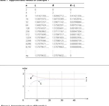
The left- and the right-hand sides of (.), respectively expressed asLandR, are shown in Table and plotted in Figure , wherea=b= .
Table 1 Approximate values of Example 1
n L R R–L
2 0 0 0
4 1 2 1
8 1.41421356. . . 1.82842712. . . 0.41421356. . .
16 1.53073372. . . 1.64725389. . . 0.11652016. . .
32 1.56072257. . . 1.59071142. . . 0.02998884. . .
64 1.56827424. . . 1.57582591. . . 0.00755166. . .
128 1.57016557. . . 1.57205691. . . 0.00189133. . .
256 1.57063862. . . 1.57111167. . . 0.00047304. . .
512 1.57075690. . . 1.57087517. . . 0.00011827. . .
1,024 1.57078647. . . 1.57081603. . . 0.00002956. . .
2,048 1.57079386. . . 1.57080125. . . 0.00000739. . .
4,096 1.57079571. . . 1.57079755. . . 0.00000184. . .
8,192 1.57079617. . . 1.57079663. . . 0.00000046. . .
. . .
. . .
. . .
. . . ∞ 1.57079632. . . 1.57079632. . . 0
3 Triangular triple integral in the 3D space
Two kinds of combined and antisymmetric finite area element vectors in the D space are reviewed in Section .. The triple integral for a -variable function is shown in Section .. Component representation and an example of it for a -variable function are shown in Section .. In the following, the Cartesian coordinates are denotedx=x,x=y, and
x=z.
3.1 Two kinds of finite area element vectors in the 3D space
For a triangular triple integral, the following increments of the double sequence of points in the D space are introduced.
. The increments of the double sequence of points at (j,k) are denoted as follows:
j
xαj,k≡xαj,k–xαj–,k, (.)
k
xβj–,k≡xβ
j–,k–
xβ
j–,k–, (.)
k
xαj,k≡xαj,k–xαj,k–, (.)
j
xβ
j,k–≡
xβ
j,k––
xβ
j–,k– (.)
forα,β= , , andj= , , . . . ,kandk= , , . . . ,n. The first combined finite area element vector (σαβ)
j,kforα,β= , , andj= , , . . . ,k andk= , , . . . ,nis introduced as
σαβj,k=j
xαj,kk
xβj–,k–k
xαj,kj
xβj,k–. (.)
. The increments of the double sequence of points at (k,j) are denoted as follows:
k
xαk,j≡xαk,j–xαk–,j, (.)
j
xβk–,j≡xβk–,j–xβk–,j–, (.)
j
xα
k,j≡
xα
k,j–
xα
k,j–, (.)
k
xβk,j–≡xβk,j––xβk–,j– (.)
forα,β= , , andj= , , . . . ,kandk= , , . . . ,n.
The second combined finite area element vector (σαβ)
k,j forα,β = , , and j= , , . . . ,kandk= , , . . . ,nis introduced as
σαβk,j=k
xαk,jj
xβk–,j–j
xαk,jk
xβk,j–. (.)
The antisymmetric symbol in the D space is
εαβγ =εαβγ = ⎧ ⎪ ⎪ ⎨ ⎪ ⎪ ⎩
+ for even permutation of{, , },
– for odd permutation of{, , },
otherwise.
(.)
Using the antisymmetric symbol in (.), the first antisymmetric finite area element vector (σ
μ= , , andj= , , . . . ,kandk= , , . . . ,nare respectively introduced as
σμ
j,k= εαβμ
σαβ
j,k, (.)
σμ
k,j= εαβμ
σαβk,j, (.)
where the indices are summed overα,β= , , .
. The first antisymmetric finite area element vector (σμ)j,k for μ= , , and j= , , . . . ,kandk= , , . . . ,nis expressed as
σμ
j,k= εαβμ
j
xα
j,kk
xβ
j–,k–k
xα
j,kj
xβ
j,k–
, (.)
where the indices are summed overα,β= , , . In detail, (.) forμ= , , are respec-tively written as
σx
j,k=
(jyj,kkzj–,k–kyj,kjzj,k–)
–
(jzj,kkyj–,k–kzj,kjyj,k–), (.)
σy
j,k=
(jzj,kkxj–,k–kzj,kjxj,k–)
–
(jxj,kkzj–,k–kxj,kjzj,k–), (.)
σz
j,k=
(jxj,kkyj–,k–kxj,kjyj,k–)
–
(jyj,kkxj–,k–kyj,kjxj,k–). (.)
. The second antisymmetric finite area element vector (σ
μ)k,jforμ= , , andj= , , . . . ,kandk= , , . . . ,nis expressed as
σμ
k,j= εαβμ
k
xαk,jj
xβk–,j–j
xαk,jk
xβk,j–, (.)
where the indices are summed overα,β= , , . In detail, the equations in (.) forμ= , , are respectively written as
σx
k,j=
(kyk,jjzk–,j–jyk,jkzk,j–)
–
(kzk,jjyk–,j–jzk,jkyk,j–), (.)
σy
k,j=
(kzk,jjxk–,j–jzk,jkxk,j–)
–
(kxk,jjzk–,j–jxk,jkzk,j–), (.)
σz
k,j=
(kxk,jjyk–,j–jxk,jkyk,j–)
–
For example, we consider the case that the boundary of the domain is a sphere:
x+y+z=a, (.)
wherea> . The following is shown inThe divergence theorem of a triangular integral[]. . The Cartesian coordinates (xj,k,yj,k,zj,k) of the antisymmetric first finite area element vector (σ
μ)j,kforμ= , , andj= , , , . . . ,kandk= , , , . . . ,non the surface of the sphere (.) are respectively expressed as
xj,k=asinθjcosϕk, yj,k=asinθjsinϕk, zj,k=acosθj, (.)
where angular arithmetic sequencesθjandϕkare respectively
θj=
j
nπ, ϕk=
k
nπ. (.)
. The Cartesian coordinates (xk,j,yk,j,zk,j) of the antisymmetric second finite area ele-ment vector (σμ)k,jforμ= , , andj= , , , . . . ,kandk= , , , . . . ,non the surface of the sphere (.) are respectively expressed as
xk,j=asinθkcosϕj, yk,j=asinθksinϕj, zk,j=acosθk, (.)
where angular arithmetic sequencesθkandϕjare respectively
θk=
k
nπ, ϕj=
j
nπ. (.)
3.2 Triangular triple integral for a 3-variable function
Assume that D is a domain and∂D is the boundary of the domain in the D space, expressed in the Cartesian coordinates (x,y,z)∈R. Let X=X=X(x,y,z), X =Y =
Y(x,y,z), andX=Z=Z(x,y,z) be partially differentiable functions with respect tox=x,
x=y, andx=zinD. There are ! = kinds of the double sequences
Xμj,k= (Xj,k,Yj,k,Zj,k), (.)
Xμk,j= (Xk,j,Yk,j,Zk,j) (.)
forμ= , , andj= , , , . . . ,kandk= , , , . . . ,n. There are two alternatives for decom-position of two kinds of double sequences (Xμ)
j,kand (Xμ)k,jforμ= , , andj= , , . . . ,k. As mentioned in the Introduction, the inappropriate two sets of increments, used in the previous article [], are replaced by the appropriate kind of two sets of incre-ments{h(xγ),h,i(xγ)i,k} and{h(xγ)h,,i(xγ)k,i} forγ = , , andi= , , . . . ,jand
h= , , . . . ,kandk= , , . . . ,nto calculate the numerical values in Example .
The following formulae have been revised based on the appropriate set of increments. In order to prove Theorem , (Xμ)
j,k and (Xμ)k,jforμ= , , andj= , , . . . ,kandk= , , . . . ,nare respectively modified in Lemmata and .
. The total increments of (Xμ)
,hforμ= , , andh= , , . . . ,kare denoted
h
Xμ
,h≡
Xμ
,h–
Xμ
,h–
=Xμ(x,h,y,h,z,h) –Xμ(x,h–,y,h–,z,h–). (.)
The increments of (xγ)
,hforγ = , , andh= , , . . . ,kare denoted
h
xγ
,h≡
xγ
,h–
xγ
,h–. (.)
The sets of possible partial increments of (Xμ)
,hforμ= , , andh= , , . . . ,kare de-noted
Xμ[hx,h] =Xμ(x,h,y,h,z,h) –Xμ(x,h–,y,h,z,h), (.)
Xμ[hy,h] =Xμ(x,h–,y,h,z,h) –Xμ(x,h–,y,h–,z,h), (.)
Xμ[
hz,h] =Xμ(x,h–,y,h–,z,h) –Xμ(x,h–,y,h–,z,h–). (.)
. The total increments of (Xμ)
i,k forμ= , , andi= , , . . . ,jandk= , , . . . ,nare denoted
i
Xμi,k≡Xμi,k–Xμi–,k
=Xμ(xi,k,yi,k,zi,k) –Xμ(xi–,k,yi–,k,zi–,k). (.)
The increments of (xγ)
i,kforγ = , , andi= , , . . . ,jandk= , , . . . ,nare denoted
i
xγi,k≡xγi,k–xγi–,k. (.)
The sets of possible partial increments of (Xμ)
i,k forμ= , , andi= , , . . . ,jandk= , , . . . ,nare denoted
Xμ[
ixi,k] =Xμ(xi,k,yi,k,zi,k) –Xμ(xi–,k,yi,k,zi,k), (.)
Xμ[iyi,k] =Xμ(xi–,k,yi,k,zi,k) –Xμ(xi–,k,yi–,k,zi,k), (.)
Xμ[izi,k] =Xμ(xi–,k,yi–,k,zi,k) –Xμ(xi–,k,yi–,k,zi–,k). (.)
Lemma In the case of(j,k)forμ= , , and j= , , . . . ,k and k= , , . . . ,n,the following
holds:
Xμj,k=Xμ,+
k
h=
Xμ[
h(xγ),h]
h(xγ),h
h
xγ,h
+ j
i=
Xμ[
i(xγ)i,k]
i(xγ)i,k
i
xγi,k, (.)
Proof Using (.) and (.), (Xμ)
j,kforμ= , , andj= , , . . . ,kandk= , , . . . ,nis split into
Xμ
j,k=
Xμ
,+ k
h=
h
Xμ
,h+ j
i=
i
Xμ
i,k. (.)
. Substituting (.), (.), and (.) into (.) forμ= , , andh= , , . . . ,k, we obtain
h
Xμ
,h=X
μ[
hx,h] +Xμ[hy,h] +Xμ[hz,h]
=X
μ[
h(xγ),h]
h(xγ),h
h
xγ
,h, (.)
where the index is summed overγ = , , .
. Substituting (.), (.), and (.) into (.) forμ= , , andi= , , . . . ,jand
k= , , . . . ,n, we obtain
i
Xμi,k=Xμ[ixi,k] +Xμ[iyi,k] +Xμ[izi,k]
=X
μ[
i(xγ)i,k]
i(xγ)i,k
i
xγi,k, (.)
where the index is summed overγ = , , .
Substituting (.) and (.) into (.), we obtain (.).
Lemma In the case of(k,j)forμ= , , and j= , , . . . ,k and k= , , . . . ,n,the following
holds:
Xμk,j=Xμ,+
k
h=
Xμ[
h(xγ)h,]
h(xγ)h,
h
xγh,
+ j
i=
Xμ[
i(xγ)k,i]
i(xγ)k,i
i
xγk,i, (.)
where the index is summed overγ = , , .
Proof In a similar manner as Lemma , we obtain (.).
Our triangular double and triple integrals and the divergence theorem in the D space are shown as follows.
Definition The triangular area double integral in the D space∂DXμdσ
μis defined
as
∂D
Xμdσμ= lim
n→∞ n
k= k
j=
Xμj,kσμ
j,k+
Xμk,jσμ
k,j
, (.)
where∂Dis the boundary of a domain,dσ
μis the antisymmetric infinitesimal area
Definition The triangular triple integral for integrands of which are partial differentials in the D spaceD∂∂Xxγμdxγdσμis defined as
D
∂Xμ
∂xγ dx
γ
dσμ
= lim n→∞
n
k= k
j=
k
h=
Xμ[
h(xγ),h]
h(xγ),h
h
xγ,h
+ j
i=
Xμ[
i(xγ)i,k]
i(xγ)i,k
i
xγi,kσμ
j,k
+
k
h=
Xμ[
h(xγ)h,]
h(xγ)h,
h
xγh,
+ j
i=
Xμ[
i(xγ)k,i]
i(xγ)k,i
i
xγk,iσμ
k,j
, (.)
whereDis a domain and the indices are summed overγ,μ= , , .
The following proposition is necessary for the condition (.) in Theorem .
Proposition Denote constants as C=Cx,C=Cy,and C=Cz,then
Cμ
∂D
dσμ=Cμ lim
n→∞ n
k= k
j=
σμ
j,k+
σμ
k,j
(.)
holds,where the index is summed overμ= , , .
Proof The proof of this proposition is shown inThe divergence theorem of a triangular
integral[].
The following is the revised version of the theorem shown inThe divergence theorem of
a triangular integral[].
Theorem (The divergence theorem of the triangular integral in the D space) Assume
that D is a domain and∂D is the boundary of the domain in theD space,expressed in the
Cartesian coordinates(x,y,z)∈R.Let Xμforμ= , , be a set of partially differentiable
functions with respect to xνforν= , , in D,where Xμ=Xμ(xν).In the case of a closed
D surface which satisfies
Cμ
∂D
dσμ= , (.)
the divergence theorem of the triangular integral in theD space holds:
—
∂D
Xμdσμ=
D
∂Xμ
∂xγ dx
γ
dσμ, (.)
Proof Combining (.) with (.) and combining (.) with (.) forj= , , . . . ,kand pressed as (.) by Definitions and under the condition of a closed surface (.).
The triangular triple integral for a -variable functionq=q(x,y,z) in the D space by the infinitesimal volume elementdV is given by
+ j
i=
qxαj,k,xβj,k,xγi,ki
xγi,k
σγ
j,k
+
k
h=
qxαk,j,xβk,j,xγh,h
xγh,
+ j
i=
qxαk,j,xβk,j,xγk,ii
xγk,i
σγ
k,j
(.)
forα=β,β=γ,γ =α, andα,β= , , as the indices of variable of functionq=q(x,y,z), whereDis a domain and the index is summed overγ= , , .
The revised corollary shown below derived from Theorem is the D version of Corol-lary .
Corollary (A corollary of Theorem ) Assume that D is a domain and∂D is the
bound-ary of the domain in theD space,expressed in the Cartesian coordinates(x,y,z)∈R.Let
Xμforμ= , , be a set of partially differentiable functions with respect to xνforν= , ,
in D,where Xμ=Xμ(xν).In the case of
—
∂D
Xμdσμ=
D
q dV, (.)
where q=q(x,y,z)is a-variable function and the index is summed overμ= , , ,the
following holds:
∂Xμ
∂xμ =q. (.)
Proof Substituting (.) and (.) into (.), it is rewritten as
D
∂Xμ
∂xγ dx
γdσ
μ=
D
q dxγdσ
γ, (.)
where the indices are summed overγ,μ= , , . Substituting (.) and (.) into (.), it is expressed as
lim n→∞
n
k= k
j=
k
h=
Xμ[
h(xγ),h]
h(xγ),h
h
xγ,h
+ j
i=
Xμ[
i(xγ)i,k]
i(xγ)i,k
i
xγi,k
εαβμ
σαβ
j,k
+
k
h=
Xμ[
h(xγ)h,]
h(xγ)h,
h
xγh,
+ j
i=
Xμ[
i(xγ)k,i]
i(xγ)k,i
i
xγk,i
εαβμ
σαβ
k,j
= nlim→∞
n
k= k
j=
k
h=
qxαj,k,xβj,k,xγ,hh
+ value of integral variables, the following ×! = kinds of formulae in two categories are required.
(.), they are reduced to the differential equation (.).
3.3 Component representation and an example of it for a 3-variable function
The left-hand side of (.) is expressed as
In component representation, (.) is expressed as
Using (.) in Definition , each component of (.) is
In Corollary , (.) is expressed as
—
and (.) is expressed as
∂X
We show an example of Corollary in the following.
Example In the case of
Substituting (.) into (.), we obtain
q(x,y,z) =x+y+z. (.)
The boundary of the domain is a sphere (.).
SinceX,= ,Y,= , andZ,= , (.) satisfies the condition of a closed surface
See (B.), (B.), and (B.) in Appendix for calculations in detail. The value of the right-hand side of (.) is
See (B.), (B.), and (B.) in Appendix for calculations in detail. We thus see the coincidence of the value of (.) and that of (.).
We consider the following approximation formula of (.) for n<∞:
In the case ofn→ ∞, (.) coincides with (.). It is verified by (.) and (.) in Example . An approximation formula, see (.), for Example is
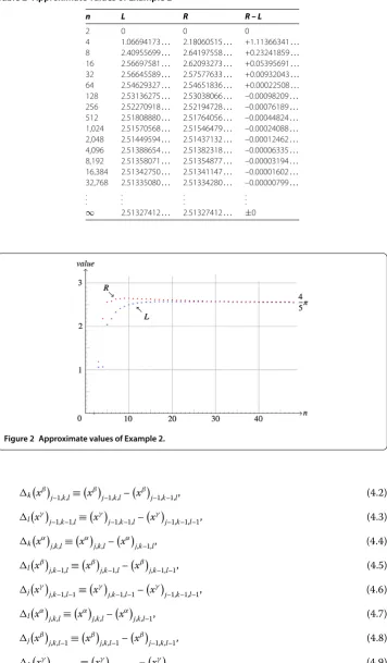
The left- and the right-hand sides of (.), respectively expressed asLandR, are shown in Table and plotted in Figure , wherea= .
4 Triangular integral in the 4D time-space
Six kinds of combined and antisymmetric finite hyper-surface element vectors in the D time-space are reviewed in Section .. The triangular quadruple integral for a -variable function is shown in Section .. In the following, the Cartesian coordinates are denoted
x=t,x=x,x=y, andx=z.
4.1 Six kinds of finite hyper-surface element vectors in the 4D time-space
For the triangular quadruple integral, the following increments of a triple sequence of points in the D time-space are introduced.
. The increments of a triple sequence of points at (j,k,l) are denoted as follows:
j
Table 2 Approximate values of Example 2
n L R R–L
2 0 0 0
4 1.06694173. . . 2.18060515. . . +1.11366341. . .
8 2.40955699. . . 2.64197558. . . +0.23241859. . .
16 2.56697581. . . 2.62093273. . . +0.05395691. . .
32 2.56645589. . . 2.57577633. . . +0.00932043. . .
64 2.54629327. . . 2.54651836. . . +0.00022508. . .
128 2.53136275. . . 2.53038066. . . –0.00098209. . .
256 2.52270918. . . 2.52194728. . . –0.00076189. . .
512 2.51808880. . . 2.51764056. . . –0.00044824. . .
1,024 2.51570568. . . 2.51546479. . . –0.00024088. . .
2,048 2.51449594. . . 2.51437132. . . –0.00012462. . .
4,096 2.51388654. . . 2.51382318. . . –0.00006335. . .
8,192 2.51358071. . . 2.51354877. . . –0.00003194. . .
16,384 2.51342750. . . 2.51341147. . . –0.00001602. . .
32,768 2.51335080. . . 2.51334280. . . –0.00000799. . .
. . .
. . .
. . .
. . . ∞ 2.51327412. . . 2.51327412. . . ±0
Figure 2 Approximate values of Example 2.
k
xβj–,k,l≡xβj–,k,l–xβj–,k–,l, (.)
l
xγj–,k–,l≡xγj–,k–,l–xγj–,k–,l–, (.)
k
xα
j,k,l≡
xα
j,k,l–
xα
j,k–,l, (.)
l
xβj,k–,l≡xβj,k–,l–xβj,k–,l–, (.)
j
xγ
j,k–,l–≡
xγ
j,k–,l––
xγ
j–,k–,l–, (.)
l
xαj,k,l≡xαj,k,l–xαj,k,l–, (.)
j
xβj,k,l–≡xβj,k,l––xβj–,k,l–, (.)
k
xγ
j–,k,l–≡
xγ
j–,k,l––
xγ
j–,k–,l– (.)
The first combined finite hyper-surface element vector (Vαβγ)
j,k,lforα,β,γ = , , , andl= , , . . . ,jandj= , , . . . ,kandk= , , . . . ,nis introduced as
Vαβγ
j,k,l= –j
xα
j,k,lk
xβ
j–,k,ll
xγ
j–,k–,l
–k
xαj,k,ll
xβj,k–,lj
xγj,k–,l–
–l
xαj,k,lj
xβj,k,l–k
xγj–,k,l–. (.)
. The increments of a triple sequence of points at (j,l,k) are denoted as follows:
j
xα
j,l,k≡
xα
j,l,k–
xα
j–,l,k, (.)
l
xβj–,l,k≡xβj–,l,k–xβj–,l–,k, (.)
k
xγj–,l–,k≡xγj–,l–,k–xγj–,l–,k–, (.)
l
xα
j,l,k≡
xα
j,l,k–
xα
j,l–,k, (.)
k
xβj,l–,k≡xβj,l–,k–xβj,l–,k–, (.)
j
xγ
j,l–,k–≡
xγ
j,l–,k––
xγ
j–,l–,k–, (.)
k
xαj,l,k≡xαj,l,k–xαj,l,k–, (.)
j
xβj,l,k–≡xβj,l,k––xβj–,l,k–, (.)
l
xγj–,l,k–≡xγj–,l,k––xγj–,l–,k– (.)
forα,β,γ= , , , andl= , , . . . ,jandj= , , . . . ,kandk= , , . . . ,n. The second combined finite hyper-surface element vector (Vαβγ)
j,l,k for α,β,γ = , , , andl= , , . . . ,jandj= , , . . . ,kandk= , , . . . ,nis introduced as
Vαβγ
j,l,k= –j
xα
j,l,kl
xβ
j–,l,kk
xγ
j–,l–,k
–l
xαj,l,kk
xβj,l–,kj
xγj,l–,k–
–k
xαj,l,kj
xβj,l,k–l
xγj–,l,k–. (.)
. The increments of a triple sequence of points at (l,j,k) are denoted as follows:
l
xα
l,j,k≡
xα
l,j,k–
xα
l–,j,k, (.)
j
xβl–,j,k≡xβl–,j,k–xβl–,j–,k, (.)
k
xγl–,j–,k≡xγl–,j–,k–xγl–,j–,k–, (.)
j
xαl,j,k≡xαl,j,k–xαl,j–,k, (.)
k
xβl,j–,k≡xβl,j–,k–xβl,j–,k–, (.)
l
xγ
l,j–,k–≡
xγ
l,j–,k––
xγ
l–,j–,k–, (.)
k