Pattern Analysis, Tracking and Control for Autonomous Mobile Robots Using Neural Networks

(1)

(2)

JAN´

ET, JASON ANDR ´

E. Pattern Analysis, Tracking and Control for Autonomous

Vehicles with Neural Networks.

(3)

(4)

First and foremost, this work is dedicated to family: To my father, for instilling a strong work ethic and providing me with the opportunity to lead crews, as well as, master masonry and machining and, hence, balance management, design and implementation in other technical areas. The speed with which projects were successfully completed, and the shear volume of students that were trained during my tenure as coordinator of the Center for Robotics and Intelligent Machines can be directly attributed to the experiences you provided me on Dogwood Quarries and at Linton Hall Military School. To my brother, Arlen, for being an inspiration on many fronts including the balance of politics, play and work. To my youngest sister, Brie, for giving me many more reasons to brag about the Jan´et family, and some of the fondest memories a big brother could hope for. To my other sisters, Shana, Caasi, Tracy and Amy, for a lot of laughs, forgiveness of my lackluster gift-giving during the holidays, and an education one can only get from sisters. To my mother, step-parents and grandparents, for marathon phone conversations and endless support.

This work is also dedicated to my friends: To Dr. Troy A. Chase, for six great years as my best friend, confidant, lab partner and business partner. Through skydiving, various masonry and robotic projects and lab co-leadership, you were a great source of support and guidance. To everyone in HELIOS, especially Amanda G. England, Rob H. Bledsoe, Pro-fessor Philip C. Lambe and ProPro-fessor Bryan W. Laffitte, for giving that extra effort, pulling together, and functioning as a well-organized group of professionals as we demonstrated all of NASA’s lunar robotic habitation tasks for the first time in the competition’s history. You earned that first place trophy and all the media acclaim! To Sean M. Scoggins, Richard D. Michelli, William J. Wiseman, Dan S. Schudel, Aaron L. Walker, and the many, many other people that helped lead robotic projects, for a lot of fun, support and insights. Look at what we accomplished with minimal funding: a biped walking robot, the hexapod colony, modular sensors, actuators, controllers and amplifiers, various mobile robots, artificial in-telligence implementations, etc. This was a great time for me! To the faculty and staff here at NCSU, for trusting me with the responsibility of the Center, allowing me to create new courses, funding projects, and the near-free reign of equipment usage. I enjoyed the opportu-nity to help students design and build at a practical level, and I pray, for the students’ sake, that you will establish well-structured mentor programs with equipment and funding so that these and other novel projects will continue. Nothing compares to the gratification of seeing their well-deserved sense of accomplishment and pride. Nothing. I would go head-to-head with those that tried to stand in our way all over again, just to see that continue.

(5)

PERSONAL BIOGRAPHY

(6)

List of Figures

2.1 Multi-layered, feed-forward architecture. . . 7 2.2 Input data space with (overlapping) regions define input-to-hidden

connec-tivity of the RFNN. . . 8 2.3 Feature neuron, FWM, patch and overlap. Feature patch convolving with

region. . . 9 2.4 Face recognition FWM images for four regions. From top to bottom: 1) eye;

2) nose; 3) mouth; and 4) chin and jaw-line. . . 10 2.5 FEM element-to-output neuron connectivity. . . 12 2.6 Output weight matrices enable output neurons to interpret the mapping of

a feature as it is convolved with its region of the input data space. . . 13 2.7 Without an upper boundary, learning rates can grow to infinity.. . . 18 2.8 Shock conditions (a) training error increases from global minima; and (b)

slow convergence. . . 19

3.1 Tavg and F per 1000 XOR neural nets without shocking. . . 23

3.2 Tavg and F per 1000 XOR neural nets with shocking. (a) M LR = 1.

(b)M LR= 20. . . 23 3.3 Tavg and F per 1000 XOR neural nets with shocking. (a) M RI = 50.

(b)M RI = 200 . . . 24 3.4 Tavg and F per 1000 XOR neural nets with shocking. (a) M RS = 0.01.

(b)M RS = 0.5.. . . 24 3.5 Uncorrupted character configurations in the XOP problem. . . 25 3.6 Tavg and F per 50 XOP neural nets without shocking. . . 26

3.7 TavgandF per 50 XOP networks with shocking. (a)M LR= 1. (b)M LR= 20. 27

3.8 Tavg andF per 50 XOP networks with shocking. (a)M RI = 50. (b)M RI =

200. . . 27 3.9 TavgandFper 50 XOP networks with shocking. (a)M RS = 0.01. (b)M RS =

0.5.. . . 28

(12)

4.2 Sonar reading and trajectory are inherently corrupted by noise. . . 33

4.3 Room character a)Cs= 0,Cr◦ = 0◦,Ct= 0; b)Cs= 0,Cr◦ = 18◦,Ct= 10%; c)Cs= 15%,Cr◦ = 0◦, Ct= 0; d)Cs= 15%, Cr◦ = 18◦,Ct= 10%. . . 33

4.4 Random steer, random travel-length. . . 34

4.5 Geometric map, sonar data and corresponding digitized room character. . . 35

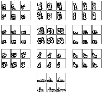
4.6 Digitized characters for Rooms 1 through 10 as observed by MARGE. . . . 35

4.7 Digitized characters for Rooms 1 through 10 as observed by Lola. . . 36

4.8 Mature features from MARGE’s neural net. . . 38

4.9 Mature features from Lola’s neural net. . . 38

4.10 Identical initial FWM weights: (1) MARGE’s matured features on left; (2) Lola’s matured features on right. . . 39

4.11 Identical initial neural network weights: (1) MARGE’s matured features on left; (2) Lola’s matured features on right. . . 39

4.12 FWM weights after total-network tuning: (1) Lola’s matured features after tuning on MARGE’s data (left); (2) MARGE’s matured features after tuning on Lola’s data (right). . . 41

5.1 Natural scene image of traffic signs.. . . 45

5.2 Training set of traffic sign images for the RFNN. . . 46

5.3 Subset of traffic signs for feature extraction. . . 49

5.4 Four analogies (matured features) from subset of traffic signs. . . 50

5.5 The only relevant analogy from the traffic sign data subset. . . 52

5.6 Testing subset of traffic sign images for the RFNN. . . 55

6.1 Using the eigenvectors ¯wkd and eigenvaluesλdextracted from the covariance matrix ¯Ck, through principal component analysis, to whiten the distribution so that ¯Ck becomes a unit matrix. . . 60

6.2 Model of cumulative distribution, ˜P_χ2(D_{M ε}). . . 62

6.3 The KS-significance parameterDKS is the difference between the theoretical distribution ˜P_χ2(D_{M ε}) and emperical distributionP(D_{M ε}). . . 63

6.4 Computed model probability for synthetically generated clusters. Contours are at 10% levels (from 10% to 90%).. . . 66

6.5 Using only the KS-test results in sporadic low significance levels. . . 68

6.6 Moving average is the average of elements inside moving window. . . 68

6.7 Applying a moving average can reduce noisy low KS-significance levels. . . 69

6.8 Model cumulative distribution, ˜P(DM εn). . . 70

(13)

6.10 Weighting the KS-significance can generally increase significance levels to more accurately reflect a node’s true compactness. . . 71 6.11 Weighting by the likelihood and applying a moving average to the

KS-significance increases KS-significance levels, reduces noise and improves discrim-ination between compact and non-compact nodes. . . 72 6.12 Squared likelihood of data-node association. . . 73 6.13 Weighting the KS-significance by the squared likelihood can generally

in-crease significance levels to more accurately reflect a node’s true compact-ness. It can also significantly improve discrimination between compact and non-compact nodes. . . 73 6.14 Weighting by the squared likelihood and applying a moving average to the

KS-significance can increase significance levels to accurately reflect a node’s true compactness. It also reduces noise and better discriminates between compact and non-compact nodes. . . 74 6.15 An obtuse V-shaped cluster modelled by a single node.. . . 81 6.16 An acute V-shaped cluster modelled by a single node. . . 81 6.17 KS-significances for obtuse and acute V-shaped clusters. Using the total

squared Mahalanobis distance shows no obvious signs of clusters being non-compact.. . . 82 6.18 Half-space KS-significances for single compact cluster on dimension,

per-polarity basis. . . 83 6.19 Half-space KS-significances for obtuse V-shaped cluster on per-dimension,

per-polarity basis. . . 83 6.20 Half-space KS-significances for acute V-shaped cluster on dimension,

per-polarity basis. . . 84 6.21 Mitosis example: cyclically splitting one node into four nodes. Contours are

90% confidence level. . . 88 6.22 Six projections of the IRIS data in Euclidean space. . . 89 6.23 IRIS data hyperellipsoids learned by the HEC Kohonen with mitosis.

El-lipses are drawn for each principal component pair, transformed into Eu-clidean space and projected onto all six viewing planes. Contours are at 90% confidence level.. . . 92

(14)

7.3 Actual sonar data collected by Lola. . . 102 7.4 25 HEC clusters and retained data points after 100 epochs of training. . . . 104 7.5 HEC cluster sets for 10 rooms using Marge’s data. . . 105 7.6 HEC cluster sets for 10 rooms using Lola’s data. . . 106

A.1 Positive and negative half-planes. . . 124 A.2 Traversability vectors for three possible paths. SG1 indicates no path

ob-struction. SG2 shows possible obstruction. SG3 shows definite obstruction. 125

A.3 Two-step t-vector test detects collisions between polygons and path segments (or single points). . . 126 A.4 T-vectors identify farthest front vertices as optimal via points. . . 129 A.5 Polyon pair with: (a) vertex t-vectors; and (b) the four half-planes that

contain either only one or both polygon(s) entirely. . . 131 A.6 Front and rear surfaces of a polygon relative tox.. . . 131 A.7 (a) Front surface is a pair of farthest front vertices. No other vertices are

(15)

Chapter 1

Introduction

Pattern analysis and control are crucial tools for autonomous vehicles. The ability to recog-nize natural landmarks from various sensors can enhance a position and orientation tracking strategy. The ability to recognize a face or voice can tell a robot who is nearby. Speech and sign-language recognition enable a robot to interpret instructions given to it through a natural medium. Character recognition enables a mobile robot tointerpretwritten land-marks (instead of memorizing the entire sign). A variety of distinctly different models exist that solve these problems individually. But if each problem required its owndedicatedmath model, a vehicle would eventually accumulate large numbers of different models, slowing access and execution. Processing engines common to multiple problems, on the other hand, would expedite pattern analysis and control, simplify execution and reduce storage require-ments. It is believed that models like the region-feature neural network (RFNN) and the hyperellipsoid clustering (HEC) Kohonen can function as such general processing engines.

Common to machine learning is the practice of feature extraction at various levels of perception. In general, feature extraction is believed to increase classification accuracy by “using only relevant attributes of the data” [88]. For self-organizing neural networks, like the HEC Kohonen, feature detection is typically based on clustering and principal component analysis (PCA) [6, 8, 50, 51, 61, 72, 75, 78, 85, 86]. For supervised learning neural networks, like the RFNN, feature detection is typically based on input-to-hidden and/or hidden-to-output synaptic weight sets from feed-forward back-propagation (backprop) architectures [5, 8, 37, 45, 47, 48, 52, 88].

(16)

1.1 The Region-Feature Neural Network

The RFNN is becoming known for its ability to perform classification, recognition, data compression and association. It is easy to implement, compact and fast. It also does not require a priori knowledge of a data point’s affiliation to a particular feature. Generally speaking, the RFNN is a multi-layered, feed-forward neural network which uses receptive fields and synaptic weight sharing to solve problems that accomodatesupervised learning. The RFNN employs “features” (receptive fields) to compensate for noise, minor phase-shifts and occlusions. The RFNN feature is a hybrid of low-level perception and computer vision morphology because the neural network autonomously learns subpatterns relevant to various classes. Once matured and determined salient, these features can be stored in long-term memory and used as “analogies” to expedite training whenever new patterns are learned or the neural network is tuned. It will be shown that analogies can develop on a small subset of classes and be used later to learn a broader set of classes. The RFNN also utilizes greedy adaptive learning rates to expedite and stabilize the overall training process. A novelad hocapproach called “shocking” is used to solve the instability problem inherent to greedy adaptive learning rates. The RFNN requires that we estimate the following: 1) the size and resolution of the input data space; 2) which regions of the input data space are important; 3) the size and overlap of the feature (receptive-field) patches; and 4) the maximum expected number of features per region.

(17)

There are several advantages to using the RFNN for supervised learning of pattern analysis and control problems. First, because the RFNN uses only one hidden layer, data requirements are minimized. Computational complexity (training and recall time) is also minimized because fewer feed-forward and back-prop calculations are needed for small ar-chitectures. Second, the RFNN has good low-level perception properties because it can autonomously learn critical features from raw or minimally pre-processed data (e.g., digital images). Third, the RFNN has good high-level perception properties because the mapping shapes the analogies (learned features stored in long-term memory) which can be used to solve a broader range of problems. Finally, the RFNN has already proven to be a reli-able pattern analysis engine despite its relatively small size and algorithmic/mathematical simplicity.

1.2 The Hyper-Ellipsoid Clustering Kohonen

The HEC Kohonen can give an autonomous vehicle a neural network with the following characteristics: 1) Self-organization; 2) Multifunctionality; 3) Small data requirements; 4) Low computational complexity; 5) Updatability; and 6) Unlimited dimensions. Few current models satisfy all of these requirements simultaneously. In this research we explore a model that incorporates the self-organizing characteristics of the Kohonen neural network [59, 60], the stochastic metric of hyper-ellipsoid clustering [13, 72, 84, 86] and the compactness of geometric environment representation [47] in a multifaceted application for autonomous vehicles.

The Kohonen neural network [60] is a well-established and widely-cited self-organizing map that learns vector-based data in an unsupervised manner. The HEC algorithm in-troduced by Mao and Jain [72] couples the Kohonen competitive learning model with the Mahalanobis distance metric to stochastically model shape information of learned clusters. Unlike the purely Euclidean distance metric (common to most Kohonen neural networks), the Mahalanobis distance can estimate shapes of elongated data in multi-dimensional data spaces. Mahalanobis contours can also measure the stochastic likelihood that a data point is associated with a particular class (node). The HEC model employs principal compo-nent analysis (PCA) to estimate the hyperellipsoidal shapes of clusters. The PCA learning algorithm is an iterative model that computes the cluster eigenvectors while ensuring or-thonormality for architectures of any dimensionality. We found the PCA model in [13, 84] to be faster and more reliable than Mao and Jain’s PCA model [72].

(18)

time-complexities, without sacrificing functionality. To add nodes we developed a mitosis algorithm which causes a parent node to divide into two daughter nodes. A compactness test determines if a node should be divided (mitosis) to better model what might actually be multiple clusters, or if a node should be pruned. The trigger mechanism for mitosis is based on this compactness of a parent node. In general, our compactness test measures how well a node’s model matches the emperical data. If a node has a learned a single cluster, it will not need to undergo midosis. On the other hand, if a node has tried to learn multiple nodes, this will be reflected by a low compactness measurement and, hence, induce mitosis.

Two commonly used tests that we considered include: 1) the Kullback-Leibler (KL) test [8]; and 2) the Kolmogorov-Smirnov (KS) test [83]. We found that both tests had very positive, yet unique properties. However, we desired more control over the sensitivity than that offered by either test by itself. Such control is needed to yield good discrimination between compact and non-compact nodes. Hence, we modified the KS-test by giving it some properities inherent to the KL-test. The resulting new KS-test allows the user to control its sensitivity by applying smoothing and/or bandpass filtering, as well as, averaging and/or likelihood weighting (raised to user-defined exponential powers). We also developed a half-space symmetry (HSS) test which can be used to detect “V”-shaped clusters. Since the compactness tests are based ondistances between a data point and a node trying to model it, V-shaped clusters can result in an inappropriate compact measure. Thus, the HSS condition looks for asymmetries about node axes to detect V-shaped clusters and induce mitosis.

(19)

1.3 Document Organization

This document is organized as follows: Chapter 2 presents the RFNN architecture, training and adaptive learning rate math models in detail. Chapter 2 also introduces the “shocking” algorithm which is used to stabilize the adaptive learning rate models. Chapter 3 validates the “shocking” algorithm on two inherently unstable benchmark problems. Chapters 4 and 5 present two implementaions of the RFNN to actual pattern analysis problems. Specifi-cally, Chapter 4 shows how an optical character recognition (OCR) approach with mapped sonar data and the RFNN can be used to solve the global self-localization (GSL) problem for autonomous mobile robots. Chapter 5 uses images of outdoor traffic signs to demon-strate a solution to outdoor landmark recognition. Both Chapters 4 and 5 demondemon-strate the concept of using previously learned features to expedite the training process, as well as transferring “knowledge” between neural networks. Chapters 4 and 5 also demonstrate how changes in the architecture (pruning and/or adding neural units and synaptic weights) do not necessarily entail a redesign penalty. Each of these implementations demonstrate how features that were matured on different data and/or on a small subset of classes can significantly reduce the training time required for learning a new and/or larger set of classes.

Chapter 6 presents the HEC Kohonen neural network architecture, training and recall algorithms in detail. All math models are furnished so that the reader can duplicate the HEC Kohonen. So that the HEC Kohonen can autonomously regulate its size, we devote a significant amount of space to the issue of measuring compactness. Specifically, we es-tablish a set of standards expected of a compactness test, and compare these to existing compactness tests. From each test we extract the elements that partially satisify these stan-dards to develop a hybrid compactness nest which allows a user to control the sensitivity to significance values. We add even greater utility to the hybrid compactness test by en-abling it to detect V-shaped clusters which might have otherwise gone undetected. Armed with a robust compactness test, we then give the HEC Kohonen the ability to add neural units through the mitosis algorithm. Removing neural units is also accomplished through pruning. We validate our models on two-dimensional synthetically generated clusters and the four-dimensional IRIS data set. In Chapter 7 we justify using the HEC Kohonen for autonomous mobile robot map building on the basis of environment representation, self-organization, updatability, unlimited dimensionality, multifunctionality, data size, complex-ity and the significant utilcomplex-ity of the stochastic measurement inherent to the HEC Kohonen. We then employ the HEC Kohonen to learn several different indoor environments using actual two-dimensional sonar data gathered from mobile robots as they explored different rooms.

(20)

(21)

Chapter 2

The Region-Feature Neural

Network

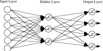
While training models like conjugate gradient back-propagation (CGBP) [11] and the Leven-berg-Marquardt (LM) algorithm [32] consistently experience fast convergences on a host of benchmark problems (both in training time and floating point operations), traditional back-propagation (backprop) is still the most popular method for neural network training. This is due in part to backprop’s mathematical simplicity as well as the vast success it has had at solving a variety of linear and non-linear problems. The basic architecture type available with the RFNN is a multi-layered feed-forward neural network because there is an input layer, hidden layer and an output layer. See Figure 2.1. This type of architecture is ideal for backprop learning.

Input Layer Hidden Layer Output Layer

Figure 2.1: Multi-layered, feed-forward architecture.

2.1 RFNN Architecture Components

(22)

receptive fields and weight sharing can compensate for slight variations in translation and rotation, using four hidden neuron layers results in long training times, increased compu-tational complexity and large data sizes [48]. The RFNN utilizes both receptive fields and weight sharing. However, unlike the OCR neural networks [64, 87], the RFNN uses only a single hidden layer. This is supported by Cybenko, who has shown that a single hidden layer is sufficient for any transformation provided enough neurons exist in the hidden layer [5].

2.1.1 Regions: Input-to-Hidden Connectivity

The input data space can be broken down into two-dimensional regions which can overlap each other or define independent portions of the data space. Figure 2.2 illustrates an example data space. Each region is defined by its minimum and maximum (row, col) locations. Figure 2.2 shows how regions define the connectivity between input layer and hidden layer neurons. Specifically, each region has its own group of hidden layer neurons. If an architecture required fully connected input-to-hidden neurons, all of the input data would be confined to one region. Otherwise, the input-to-hidden neurons can be made partially connected by breaking the data space into multiple regions.

Input Data Space Region # 1: 1,1( )min to 5,10( )max

Region #2: 4,8( )min to 7,17( )max

0.2 0.2 1.4 1.9 3.3 1.8 1.1 0.7 0.2 0.1 0.1 0.1 0.3 0.9 1.8 2.2 0.9 0.1 0.1 0.8 1.8 3.0 2.6 1.1 0.7 0.4 0.2 0.1 0.1 0.5 1.1 1.8 2.4 1.9 0.2 0.2 1.6 1.9 2.3 1.9 1.4 1.2 0.4 0.3 0.2 0.1 0.3 0.9 1.8 2.2 1.7 0.2 0.2 1.4 1.9 2.3 1.8 1.6 1.7 0.2 0.1 0.1 0.1 0.3 0.7 1.2 2.1 0.9 0.2 0.2 1.6 1.9 2.3 1.9 1.4 1.2 0.4 0.3 0.2 0.1 0.3 0.9 1.8 2.2 1.7 0.1 0.1 0.8 1.8 3.0 2.6 1.1 0.7 0.4 0.2 0.1 0.1 0.5 1.1 1.8 2.4 1.9 0.2 0.2 1.6 1.9 2.3 1.9 1.4 1.2 0.4 0.3 0.2 0.1 0.3 0.9 1.8 2.2 1.7

Region 1

Region 2

Figure 2.2: Input data space with (overlapping) regions define input-to-hidden connectivity of the RFNN.

2.1.2 Features: Hidden Neuron Kernels

(23)

featurepatchsize (kernel size). Specifically, a patch is a subset of its respective region and, hence, its size is described by the number of rows and columns (≤ the size of the region). See Figure 2.2.

0.2 0.2 1.4 1.9 3.3 1.8 1.1 0.7 0.2 0.1 0.1 0.1 0.8 1.8 3.0 2.6 1.1 0.7 0.4 0.2 0.2 0.2 1.6 1.9 2.3 1.9 1.4 1.2 0.4 0.3 0.2 0.2 1.4 1.9 2.3 1.8 1.6 1.7 0.2 0.1 0.2 0.2 1.6 1.9 2.3 1.9 1.4 1.2 0.4 0.3 0.2 0.2 1.4 1.9 3.3 1.8 1.1 0.7 0.2 0.1

0.1 0.1 0.8 1.8 3.0 2.6 1.1 0.7 0.4 0.2 0.2 0.2 1.6 1.9 2.3 1.9 1.4 1.2 0.4 0.3 0.2 0.2 1.4 1.9 2.3 1.8 1.6 1.7 0.2 0.1 0.2 0.2 1.6 1.9 2.3 1.9 1.4 1.2 0.4 0.3 0.2 0.2 1.4 1.9 3.3 1.8 1.1 0.7 0.2 0.1

0.1 0.1 0.8 1.8 3.0 2.6 1.1 0.7 0.4 0.2 0.2 0.2 1.6 1.9 2.3 1.9 1.4 1.2 0.4 0.3 0.2 0.2 1.4 1.9 2.3 1.8 1.6 1.7 0.2 0.1 0.2 0.2 1.6 1.9 2.3 1.9 1.4 1.2 0.4 0.3 Patch of Input Layer

Patch Columns

Patch Rows Feature Synaptic Weights

(Feature Weight Matrix)

Feature Bias Feature

Sigmoid Feature Element Output

Row Overlap

Column Overlap

Repositioned Feature Patch

Figure 2.3: Feature neuron, FWM, patch and overlap. Feature patch convolving with region.

FWM images show how the neural net weighs input data before it is introduced to hidden-layer neurons. As an example, Figure 2.4 shows a set of features from a four-region face recognition RFNN. Black pixels correspond toωF W MM IN, white pixels correspond to

ωF W MM AX. (ωF W MM IN is the smallest (perhaps more negative) feature-level weight when

added to its bias,ωFb, and ωF W MM AX is the largest feature-level weight when added to its

respective feature biasωFb.) From top to bottom: 1) For the eye region, the 25×50 FWM

shows a greater emphasis of weight (indicated by brighter pixels) on the eyes and a lower emphasis (indicated by darker pixels) on the areas around the eyes. 2) For the nose region, the 25×15 FWM shows an emphasis of weight on the ridge and tip of the nose. 3) For the mouth region, the 15×25 FWM shows there is less weight placed on the center of the mouth presumably because it is not a reliable area to associate with a face due to mouth movement. 4) The 15×40 FWM for the chin and jaw-line region shows that most weight is placed on the areas below and to the side of the chin and jaw-line.

2.1.2.1 Patch Size and Overlap

(24)

Figure 2.4: Face recognition FWM images for four regions. From top to bottom: 1) eye; 2) nose; 3) mouth; and 4) chin and jaw-line.

rows and 4 columns can have an overlap of as much as 2 rows in the row-direction and as much as 3 columns in the column-direction.

Another way of envisioning the role of patches is to consider the following: By using receptive fields (feature patches), we identify an entire mapped out image, time-series or data pattern by looking at smaller portions of it. To a degree, the smaller the portions, the fewer possible variations in features. However, patches that are too small ignore the collective effect of groups of data elements. For example, viewing a Picasso painting from 20 meters away can make the painting appear as a crude cluster of colors. Similarly, looking at the same Picasso painting from only 2 cm away can make the painting appear as a similar cluster of randomly placed colors. The optimal viewing position is likely somewhere in between. So the optimal size of a feature patch is somewhere between a single data element and the entire region size. It has been seen that this choice is typically problem-dependent.

(25)

use binary inputs in the problem space or, for that matter, assume that the feature kernels are binary. The binary idea is simply used as an example with finite outcomes. Analog, of course, would yield an infinite number of possible feature configurations. Furthermore, the feature kernel, trained by an averaging of errors per placement, is ultimately an analog aspect of the neural network.

2.1.2.2 Receptive Fields Compensate for Translation and Rotation

Patch overlapping can compensate for slight rotations and translations of a feature by searching areas of the region at and near the location of the expected feature occurrence. These variations might be caused by noise or a miscalibrated medium used for measuring the problem space elements. A practical example of this can be found in the optical character recognition (OCR) problem. Consider for now that we are using a black and white video camera to identify printed letters. We presently assume that one character can almost fill the image (i.e., problem space). We assume further that the image is thresholded so that the pixels are either black or white (i.e., there is no gray scale). Hence, the problem space is a binary pixel matrix that is updated each time an image is captured for analysis. Clearly it is possible that the printed letter is shifted a few pixels up or down and, for that matter, or rotated slightly. Hence, letting the feature patch shift side-to-side and up-and-down maximizes the opportunity that an important feature can, in fact, be found in the general area of where it was expected.

Looking at successive subsets of the problem space in this manner is referred to as using receptive fields. The practice of measuring these subsets with a feature whose synap-tic weights are position-independent is called receptive field weight-sharing. Choosing the number of features a particular region should have can prove to be a rather subjective and arbitrary process. One might decide, for example, that the neural net will have to look for horizontal and vertical lines and thus decide that only two features are necessary. In truth, however, this way of envisioning how the neural net will learn and identify a feature might be completely different from how the neural net actually learns and identifies a feature. After all, unlike computer vision morphology, the neural network decides for itself how a feature should be measured. It is assumed that this is because the neural net does not only look atwhethera candidate feature does or does not completely match; it also looks at the degree of match. In general, we want to minimize the number of features to minimize the overall architecture data size.

2.1.3 Feature Mapping with the FEM

(26)

Output Neuron Value

0.2 0.2 1.4 1.9 3.3 1.8 1.1 0.7 0.2 0.1 0.1 0.1 0.8 1.8 3.0 2.6 1.1 0.7 0.4 0.2 0.2 0.2 1.6 1.9 2.3 1.9 1.4 1.2 0.4 0.3 0.2 0.2 1.4 1.9 2.3 1.8 1.6 1.7 0.2 0.1 0.2 0.2 1.6 1.9 2.3 1.9 1.4 1.2 0.4 0.3

0.2 0.2 1.4 1.9 3.3 1.8 1.1 0.7 0.2 0.1 0.1 0.1 0.8 1.8 3.0 2.6 1.1 0.7 0.4 0.2 0.2 0.2 1.6 1.9 2.3 1.9 1.4 1.2 0.4 0.3 0.2 0.2 1.4 1.9 2.3 1.8 1.6 1.7 0.2 0.1 0.2 0.2 1.6 1.9 2.3 1.9 1.4 1.2 0.4 0.3 0.2 0.2 1.4 1.9 3.3 1.8 1.1 0.7 0.2 0.1

0.1 0.1 0.8 1.8 3.0 2.6 1.1 0.7 0.4 0.2 0.2 0.2 1.6 1.9 2.3 1.9 1.4 1.2 0.4 0.3 0.2 0.2 1.4 1.9 2.3 1.8 1.6 1.7 0.2 0.1 0.2 0.2 1.6 1.9 2.3 1.9 1.4 1.2 0.4 0.3

Feature Element Matrix FEM Columns

FEM Rows

FEM Element-to-Output Synaptic Weights

Output Bias Output Sigmoid

Figure 2.5: FEM element-to-output neuron connectivity.

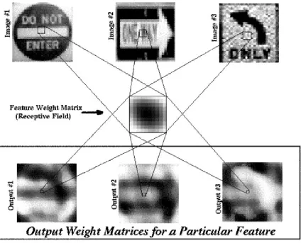
feature element matrix(FEM) which becomes, in turn, an input to the output neuron layer. Hence, a set of synapses called the output weight matrix (OWM) exists between the FEM elements and each output neuron. Each feature has its own FEM which shows the output layer where and to what degree certain sub-patterns are found. That is, output neurons can assess with an OWM the mapping of each feature. Figure 2.5 shows how a FEM is filled and then connected to an output layer neuron. The set of FEM element-to-output weights (OWM) is different for each output neuron. This is because each output neuron is entitled to place as much or as little significance on the mapping of each type of feature. After all, not all feature types are expected to be relevant to all output neurons. Graphical images of synaptic weights can be used to understand how each output neuron weighs the mapping of features in the preceeding layer. Images for OWM’s are scaled to the range [ωOW MM IN, ωOW MM AX] whereωOW MM IN is the smallest output-level weight (perhaps more

negative) when added to its bias, ωOb, and ωOW MM AX is the largest output-level weight

when added to its respective output biasωOb. Black pixels correspond toωOW MM IN, white

pixels correspond to ωOW MM AX. In the context of the traffic sign recognition problem,

Figure 2.6 pictoralizes how OWM’s weigh the elements of a FEM.

2.1.4 Number and Function of Output Layer Neurons

(27)

(28)

the input data pattern with that particular output neuron. Of course, the infinite number of possible neuron values in the rangef(neto)∈[0,1] can be used to measure the degree of

association.

2.1.5 Analogies: Mature Feature Preservation

The RFNN software allows for the preservation of matured features, referred to asanalogies. Loading previously learned features gives a new or modified neural net “prior knowledge” in the training process. By definition, a feature is an aspect, quality or characteristic that is unique to a particular process, pattern, image, etc. Once learned, a basic feature remains fairly constant...“red” is “red” no matter its context. Re-learning a feature that can be useful to a variety of classes or problem domains wastes training time and data storage. When a neural network uses features previously learned by other neural networks, we lock the features to ensure that the training process does not change the synaptic weights unique to that feature. The only synaptic weights thatcan change during training are hidden-to-output weights (OWM’s) and the input-to-hidden weights of featuresnotused as analogies. Algorithmically, the overall training process is expedited with analogies because there are fewer synaptic weights to update. This is significant to a variety of problems because the time spent learning new classes or domains can, therefore, be significantly reduced.

2.2 The RFNN Backprop Training Algorithm

Due to the uniqueness of receptive-field architectures and weight sharing, the back-propagation training algorithm must be adapted to the RFNN. For an architecture withr= 1,2, ..., R re-gions, therthregion is defined in the data space byr∈[(rowr_min, colr_min),(rowr_max, colr_max)]. For each regionr there aref = 1,2, ..., Fr features each of patch size Psizer = (NP

r

rows, NP

r

cols)

and overlapOr_size= (N_rowsOr , N_colsOr). Hence, for each feature f the FEM size is F EMr,f_size= (N_rowsF EMr,f, N_colsF EMr,f) where,

N_rowsF EMr,f =

$

rowr

max−rowminr −NO

r

rows+ 1

NPr

rows−NO

r

rows

%

(2.1)

N_colsF EMr,f =

$

colr_max−colr_min−N_colsOr + 1 N_colsPr −N_colsOr

%

(2.2)

and the FWM of input-to-hidden synaptic weights is

F W Mr,f =

ω₁r,f_,₁ . . . ωr,f

1,NP r cols

..

. . .. ...

ωr,f_NP r

rows,1 . . . ω

r,f

NP r

rows,NcolsP r

(29)

where each synaptic weight,ωr,f

m,n corresponds to themth row andnthcolumn of the FWM

belonging to featuref in region r. Also, each feature has a bias weight,ωr,f_b . Each element of F EMr,f is filled by the standard sigmoidal measurement

f(neti,j) =

1

(1 + exp−neti,j₎ (2.4)

whereiand j are indices (which begin at (1, 1)) ofF EMr,f and

neti,j =

NP r

rows

X

m

NP r

cols

X

n

ω_m,nr,f ax,y

+ω_br,f. (2.5)

The term ax,y is the value of an input element from the data space inside region r. The

indices x and y (which also begin at (1, 1)) represent the row and column, respectively, of the input element with respect to the input data space. Consequently,

x=hrow_minr + (i)N_rowsPr −N_rowsOr +mi, y=hcolr_min+ (j)N_colsPr −N_colsOr+ni (2.6)

If, as is the case with the RFNN, the neural network is fully connected between the feature element matrices and output neurons, there exists a synaptic weight between every output neuron and every cell of every FEM. This gives the RFNN a tendency to be top-heavy. Since each output neuron considers the value associated with each placement of the feature patch, there can be significantly more FEM element-to-output neuron synapses than input-to-feature neuron synapses. So each output neuron o = 1,2, . . . , O assumes a value according to the sigmoid

f(neto) =

1

(1 + exp−neto₎ (2.7)

where,

neto= R

X

r

Fr

X

f

NF EM r,f rowsX

i

NF EM r,f colsX

j

h

ωo_r,f,i,jF EM(i, j)i+ω_bo. (2.8)

Although this notation seems more complicated than other fully connected feed-forward neural networks [89], it allows us to construct architectures with receptive fields and weight sharing [63, 64, 87]. If an architecture does not need receptive fields, the RFNN patch is the same size as the region. This makes the FEM matrices only one element in size. Hence, this notation lends greater flexibility to neural network architectures by giving the option of using receptive fields.

(30)

movable feature patch. Since feature patches are not necessarily fixed over the problem space, each individual synapse can be affected by a multitude of input values per data exampleq= 1,2, . . . , Q. From [37], the task of the network is to learn associations between a specified set of input-output pairs np₁, t1

,p₂, t2

, . . . ,p_Q, tQ

o

. The performance index for the network is

ˆ V = 1

2

Q

X

q

o_q−t_qT o_q−t_q= 1 2

Q

X

q

eT_qe_q (2.9)

where o_q is the vector of output neuron values resulting from the qth input, p_q, and e_q=o_q−t_q is the error for the qth input. For the standard back-propagation algorithm we use an approximate steepest descent rule. For a single input/output pair the performance index can be approximated by ˆVq = 1₂eTqeq. For epoch k = 1,2, . . . , K the approximate

steepest (gradient) descent algorithm for the FEM element-to-output neuron synapse and output neuron bias weights require that

ω_r,f,i,jo (k+ 1) =ω_r,f,i,jo (k)−αo_r,f,i,j(k)

Q

X

q

∂Vˆq(k)

∂ωo

r,f,i,j(k)

(2.10)

and

ω_bo(k+ 1) =ωo_b(k)−α_bo(k)

Q

X

q

∂Vˆq(k)

∂ωo_b(k) (2.11)

where αo_r,f,i,j(k) and αo_b(k) are the adaptive learning rates at epoch k for the individual FEM element-to-output neuron synapses and output bias synapses respectively. Similarly, the steepest descent algorithm for feature biases require that

ω_br,f(k+ 1) =ωr,f_b (k)−α_br,f(k)

Q

X

q

∂Vˆq(k)

∂ω_br,f(k) (2.12)

Unlike the fairly standard synaptic weight update rules of 2.10 to 2.12, the feature patch synaptic weights (FWM) must be updated to account for every placement in the region. Hence,

ω_m,nr,f (k+ 1) =ωr,f_m,n(k)−αr,f_m,n(k)

Q

X

q

NF EM r,f rowsX

i

NF EM r,f colsX

j

∂Vˆq(k)

∂ωm,nr,f,i,j(k)

(2.13)

2.3 The Modified Adaptive Learning Rate Model

(31)

is because each synapse has its own learning rate that varies over time. It has been shown that “the method of adaptive learning rates is much faster than steepest descent, generally reducing training time by an order of magnitude, and it is also very dependable. It is not prone to get into trouble and does not require special care...[It] is fast, dependable, and highly automatic...” [89]. The adaptive learning rate modification proposed by Jacobs [38] has become popular for two main reasons: minimal mathematical complexity and numerous reported successes at achieving faster convergences.

The adaptive learning rate model is based on four heuristics that suggest that each weight of a neural network should have its own learning rate and that these rates be al-lowed to change over time. Qualitatively, the heuristics are: 1) Every parameter of the performance measure should have its own individual learning rate; 2) Every learning rate should be allowed to vary over time; 3) When the derivative of a parameter possesses the same sign for consecutive time steps, the learning rate for that parameter should be in-creased; and 4) When the sign of the derivative of a parameter alternates for consecutive time steps, the learning rate for that parameter should be decreased. The math model for these heuristic rules are presented below. In general, each synaptic weight in a neural network architecture is allowed to have its own learning rate. We are concerned with the direction in which errors for a synaptic weight decrease over an exponential averagefω,

fω(k+ 1) =θ·fω(k) + (1−θ)dω(k) (2.14)

where dω(k) = PQq

∂Vˆq(k)

∂ω(k) and θ defines the weighting of consecutive error associations

(θ≈0.1). The signs of dω and fω give us a precise measure of the direction in which the

error decreases both currently and recently. The equation for the adaptive learning rate of a synaptic weight, is

αω(k+ 1) =

(

αω(k)·κ ifdω(k)fω(k)>0 andαω(k)< τ

αω(k)·φ ifdω(k)fω(k)≤0 (2.15)

where typicallyκ≈1.1 and φ≈0.5.

Despite their success at reducing training times, adaptive learning rate models tend to create instabilities which can cause a neural network to saturate1 _{[37]. We recall that the}

standard backprop model estimates the error associated with a synaptic weight to prescribe a weight change. Typically, the synaptic weight is updated by only a fraction (less than unity) of the prescribed weight change. While this suggests an inherent stability in the overall weight update method, it also causes training times to be slow. On the other

1

(32)

hand, updating a synaptic weight by more than the prescribed weight change (learning rate greater than unity) can significantly reduce training times. However, this “greedy” approach increases the likelihood of instabilities.

One extremely important difference between equation 2.15 and the adaptive learning rate method in [38] should be noted; instead of adding κ ≈ 0.1 to the learning rate, we multiply κ ≈ 1.1 [94]. The need to do this stems from the fact that architectures with many synapses can saturate if their learning rates are too high. In fact, extremely large architectures can have initial learning rates on the order of αω(0) ≈ 0.0001. Hence, an

additionofκ≈0.1 toαω would have too radical an effect on the back-propagation process.

Instead, a subtle 10% increase of the learning rate each epoch reduces the tendency toward saturation regardless of the initial learning rate magnitude [94].

lr_init=0.1 lr_init=0.01 lr_init=0.001

0 10 20 30 40 50 60 70 80 90 100 0

1 2 3 4 5 6 7 8 9 10

Epoch

Learning Rate

Learning Rates vs Epoch for Adaptive Learning Rate Rule

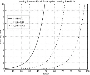
Figure 2.7: Without an upper boundary, learning rates can grow to infinity.

Another very important detail from equation 2.15 not mentioned in [38] is that an upper bound τ must be placed on αω. If dω(k)fω(k) > 0 and αω(k) < τ the learning rate can

grow to infinity. Figure 2.7 shows the learning rate change according to equation 2.15 for three different initial learning rates (αω(0) ∈ {0.1,0.01,0.001}). Typically, τ ≤ 1 since

(33)

2.4 Heuristics for Shocking Adaptive Learning Rates

Our research indicates that it is possible to let learning rates become greedy τ > 1 and still maintain stable convergence. This is accomplished through an ad hocapproach called “shocking” [2, 43, 44]. Simply stated, shocking a neural network reduces all synaptic learn-ing rates to small values. The two conditions for shocklearn-ing are heuristic, yet they can be justified and they have a proven significant impact on the reduction of failure rates. The first heuristic condition stipulates that if the training error at epoch k+ 1 increases to a value larger than the error at epoch k, the neural net should be shocked. See Figure 2.8a.

Reverting to small learning rates gives the neural net the opportunity to quickly (re)turn to its original destination or, due to the instability that triggered the shock, locate a better minima on the error surface.

Epochs 50

0 k k+1

(a) (b)

Epochs 50 0

∆k

∆

MRI

kshock k k+1

ˆ

V _Vˆ

ˆ

V

k

∆Vˆ

∆k<τ∆Vˆ

∆

Figure 2.8: Shock conditions (a) training error increases from global minima; and (b) slow convergence.

The second heuristic condition for shocking requires that if the learning rates are large enough to significantly impact training, but the training error is decreasing at a very slow rate ∆ ˆ_∆V_k, the neural net should be shocked. See Figure 2.8b. The reason for this is as follows: When the learning rates are very large, it is possible for the synaptic weights to overshoot and vacillate over a minima while still very slowly converging and not causing the neural net to saturate [94]. As a part of this condition we specify that the learning rates should be large because they need time to grow enough to significantly impact the convergence. Hence, we can restate the second condition with,if a number of epochs have elapsed∆k=k−kshock since the last time the net was shocked ∆k≥M RI (minimum reset

interval) and the training error is decreasing at a rate less than a specified minimum reset

slope, ∆ ˆ_∆V_k ≤τ∆ ˆV

∆k

, then the neural net should be shocked.

(34)

that converge, the average training times with shocking will typically not be less than the average training times for neural networks without shocking. This is expected since the conditions for shocking are sensitive to instabilities regardless of magnitude. Hence, the neural network loses some momentum each time the learning rates are reset. But the advantage of shocking lies more in its effectiveness at improving a neural network’s probability of convergence even when the learning rates become very large. In [44] it is shown that shocking reduces the number of failed convergences for the XOR problem by as much as 33%. Also in [44], for the problem of classifying 3x3 ’×’, ’’ and ’+’ characters in a 5x6 image, the number of failed convergences decreased by as much as 100%.

2.5 Normalized Learning

One learning method that can be used to train a neural network is that ofnormalized learn-ing[18]. Briefly speaking, normalized learning finds the largest prescribed synaptic weight change at the end of each epoch and sets it equal to themaximum weight change (MWC) allowable for that epoch. The remaining prescribed weight changes are then proportionally scaled to their respective fractions of the MWC. So if the largest recommended synaptic weight change issmallerthan theMWC, all of the recommended weight changes are scaled up. If the largest recommended synaptic weight change islargerthan theMWC, all of the recommended weight changes are scaled down. The MWC is decayed at an exponential rate on a per-epoch basis. Normalized learning is not recommended for large data spaces and/or large architectures. However, normalized learning does seem to expedite the training process for smaller problems and architectures.

2.6 Coupling Hidden-to-Output Synaptic Weights

(35)

Chapter 3

Validation of Learning Rate

Shocking

There are many parameters that determine a neural network’s training time and tendency to fail. Some of these include: 1) the type of problem being solved; 2) the architecture size; 3) the initial synaptic weights; 4) the initial learning rates; 5) the maximum learning rate; and so on. In this instance we are interested in the effects of shocking on two random variables: training timeT ∈[0,∞) and failureF ={0,1} of an architecture to converge in less than τF epochs. In this chapter, we use two inherently unstable benchmark problems:

1) the XOR problem; and 2) the XOP problem (a simple character recognition problem with ‘×’, ‘’ and ‘+’). Many other large-scale problems have taken advantage of shocking, as well [2, 43, 45, 47].

In this chapter we: 1) study the effects of placing an upper limit on adaptive learning rate values; and 2) assess the effects of learning rate shocking. To reiterate, shocking is simply resetting all synaptic learning rates to their initial values according to the two heuristic rules discussed in Section 2.4. The two random variables measured in this comparison are training time T ∈ [0,∞) and failure F = {0,1} of an architecture to converge in less than τF epochs. While there are many parameters that contribute to a neural network’s

convergence rate, we allow only three parameters to vary: 1) the maximum learning rate M LR={1, ..,20}; 2) the minimum reset intervalM RI ={50, ..,200 epochs}; and 3) the minimum reset slopeM RS ={0.01, ..,0.5 per epoch} of the training error per epoch.

3.1 The XOR Problem

(36)

little to no consideration is given to why some XOR neural nets fail to converge or, for that matter, how to reduce the chances of failure. It will be seen that shocking reduces the number of failed convergences by at least 30%.

The architecture used in this problem has the standard two-inputs, two-hidden layer neurons, single-output layer neuron (equivalent to a single 1×2 region, two-feature, single-output architecture for the RFNN). The analysis for this problem is based on 1000 2:2:1 XOR neural nets whose input-to-hidden synaptic weights are randomly initialized to values between ±0.1 and whose hidden-to-output synaptic weights are randomly initialized to values of ±1. The initial learning rate for all synaptic weights is 0.9. These parameters might or might not be “optimal”. But, due to their consistency and abundance, they provide a good basis for observing the random variables training time T and failure F of an architecture to converge in less than τF = 10000 epochs.

3.1.1 Adaptive Learning Without Shocking

We first look at the collective effects of varying the maximum learning rate M LR = {1, . . . ,20}. Figure 3.1 indicates that the average training time and variance for neural nets that converged reduced significantly with increasedM LR. The lowest average training time was 240 epochs. But the number of failed convergences ranged from 2 to 33 with a trend that increased seemingly without bound as the maximum learning rate increased.

3.1.2 Adaptive Learning With Shocking

(37)

2 4 6 8 10 12 14 16 18 20 0 10 20 30 40

# Failures vs Maximum Learning Rate

Maximum Learning Rate

# Failures

2 4 6 8 10 12 14 16 18 20

0 500 1000 1500 2000

Mean # Epochs

AL w/o Shock: Avg Training Time vs Maximum Learning Rate

Figure 3.1: Tavg andF per 1000 XOR neural nets without shocking.

50 100 150 200 0 0.05 0.1 0 1000 2000 Epochs

AL w/ Shock: Avg Training Time for MLR=1

50 100 150 200 0 0.05 0.1 0 20 40 # Failures

Min Reset Slope Min Reset Interval # Failures for MLR=1

50 100 150 200 0 0.05 0.1 0 1000 2000 Epochs

50 100 150 200 0 0.05 0.1 0 20 40 # Failures

Figure 3.2: Tavg andF per 1000 XOR neural nets with shocking. (a)M LR= 1. (b)M LR=

(38)

0 0.05 0.1 0.15 0 5 10 15 200 1000 2000 Epochs

AL w/ Shock: Avg Training Time for MRI=50

0 0.05 0.1 0.15 0 5 10 15 200 20 40

Max Learning Rate Min Reset Slope

# Failures

# Failures for MRI=50

0 0.05 0.1 0.15 0 5 10 15 200 1000 2000 Epochs

0 0.05 0.1 0.15 0 5 10 15 200 20 40

# Failures

Figure 3.3: Tavg and F per 1000 XOR neural nets with shocking. (a) M RI = 50.

(b)M RI = 200 .

50 100 150 200 0 5 10 15 200 1000 2000 Epochs

AL w/ Shock: Avg Training Time for MRS=0.01

50 100 150 200 0 5 10 15 200 20 40

Max Learning Rate Min Reset Interval

# Failures

# Failures for MRS=0.01

50 100 150 200 0 5 10 15 200 1000 2000 Epochs

50 100 150 200 0 5 10 15 200 20 40

# Failures

Figure 3.4: Tavg and F per 1000 XOR neural nets with shocking. (a) M RS = 0.01.

(39)

3.2 The XOP Problem

The XOP problem is a simple character recognition problem where the input vector is two-dimensional. Specifically, we have a 5×6 pixel binary image as our problem space upon which one of three 3×3 characters can appear: 1) ‘×’; 2) ‘’; and 3) ‘+’. It is assumed that the character can be anywhere inside the problem space and that only one character will be in the input data space at a time. The architecture used to solve the XOP problem uses 3×3 receptive fields (see Section 2) and 3 output neurons. This translates into a single region, 3 feature, 3 output RFNN. Each feature is 3×3 with a 2×2 overlap. Figure 3.5 shows some examples of XOP character configurations.

Figure 3.5: Uncorrupted character configurations in the XOP problem.

Like the XOR problem, the XOP problem is inherently unstable. In fact, we use more than just the shocking heuristic to stabilize training on the XOP problem with the afore-mentioned architecture. Specifically, it was determined that nearly all of the randomly initialized XOP architectures failed to converge unless we coupled the hidden-to-output synaptic weights1. Otherwise, the analysis for this problem is based on 50 XOP neural nets2 whose input-to-hidden synaptic weights are randomly initialized to values between ±0.001 and whose hidden-to-output synaptic weights are randomly initialized to values between ±0.0001. The initial learning rate for all synaptic weights is 0.4. Again, these parameters might or might not represent “optimal” conditions for XOP neural nets. But, they do provide a good basis for observing and modelling the random variables training timeT and failureF of an architecture to converge in less thanτF = 3000 epochs.

3.2.1 Adaptive Learning Without Shocking

By varying the maximum learning rate M LR = {1, . . . ,20}, Figure 3.6 shows that the average training time for neural nets that converged reduced significantly with increased M LR. The lowest average training time in this case was 417 epochs. The number of failed 1_{This is actually the only problem we have found to need hidden-to-output synaptic weights to be coupled.} 2

(40)

2 4 6 8 10 12 14 16 18 20 0

10 20 30 40

# Failures vs Maximum Learning Rate

Maximum Learning Rate

# Failures

2 4 6 8 10 12 14 16 18 20

0 500 1000 1500 2000

Mean # Epochs

AL w/o Shock: Avg Training Time vs Maximum Learning Rate

(41)

convergences ranged from 2 to 6. No clear trend can be extrapolated from the failure rate plot. However, it is clear that within the range of M LR = {1, . . . ,20} at least 4% of the XOP neural nets failed to converge.

3.2.2 Adaptive Learning With Shocking

Looking now at figures 3.7 through 3.9 it can be seen that the effects of varying the three parameters M RI = {50, ..,200 epochs}, M RS = {0.01, ..,0.5 per epoch}; and M LR = {1, ..,20} generally reduced the average training times with increased M LR and M RI. For each combination, there were no failures. In fact, for all of the combinations where M LR > 1, there were no failed convergences. So shocking stabilized up to 100% of the XOP neural nets that might have otherwise failed without shocking.

50 100 150 200 0 0.05 0.1 0.150 500 1000 Epochs

50 100 150 200 0 0.05 0.1 0.150 1 2 # Failures

50 100 150 200 0 0.05 0.1 0.150 500 1000 Epochs

50 100 150 200 0 0.05 0.1 0.150 1 2 # Failures

Figure 3.7: Tavg andF per 50 XOP networks with shocking. (a)M LR= 1. (b)M LR= 20.

0 0.05 0.1 0.15 0 5 10 15 200 500 1000 Epochs

0 0.05 0.1 0.15 0 5 10 15 200 1 2

# Failures

0 0.05 0.1 0.15 0 5 10 15 200 500 1000 Epochs

0 0.05 0.1 0.15 0 5 10 15 200 1 2

# Failures

Figure 3.8: Tavg and F per 50 XOP networks with shocking. (a) M RI = 50. (b)M RI =

(42)

50 100

150 200 0

5 10 15 200 500 1000

Epochs

50 100

150 200 0

5 10 15 200

1 2

# Failures

50 100

150 200 0

5 10 15 200 500 1000

Epochs

50 100

150 200 0

5 10 15 200

1 2

# Failures

Figure 3.9: Tavg andF per 50 XOP networks with shocking. (a)M RS = 0.01. (b)M RS=

0.5.

3.3 Summary on the Effects of Shocking

(43)

Chapter 4

Transferring Neural Net-Based

Knowledge Between Two Mobile

Robots

An application where the RFNN is used to recognize sensor patterns involves giving a robot the ability to determine which topographical region it is in. This chapter describes how two mobile robots can share knowledge about their environment. The two mobile robots we use have different sensor configurations, drive systems and other physical attributes including weight and size. “Knowledge” is generated by the RFNN, and can be transferred on two general levels: 1) a complete transfer of a matured neural network; and 2) a transfer of matured features. The transfered knowledge can also be “tuned” with and without locking the feature level synaptic weights. We examine the impact and feasibility of sharing (on both levels, with and without locking features) neural network modules trained on actual sonar data in the global self-localization (GSL) problem. We also describe the neural network architecture and our general approach to solving the GSL problem in a time-, translation- and rotation-invariant way. Significant reductions in training time are realized and presented.

4.1 Introduction

(44)

To date a significant amount of work has been devoted to developing self-localization approaches for autonomous mobile robots that depend on prior dead reckoning estimates and discrete-time models to rationalize and correct robot position and orientation based on correlations between predicted and actual sensor data [16, 62, 65, 71]. But, without an initial reliable position estimate, even the most proven techniques can become ineffective. Our objective is to endow mobile robots with the ability to perform self-localization on a global level. A mobile robot should be able to use sensor data to autonomously determine which region of space it is in without knowing how it got there.

4.1.1 OCR-Based Mobile Robot Global Self-Localization

We treat the sonar-based GSL of a mobile robot as an optical character recognition (OCR) problem [41, 42, 43]. Natural landmark signatures can, through mapped sonar data, assume character-like configurations unique to those landmarks. The ability to identify each room character helps a mobile robot determine its global location by association. Since most indoor environments can be easily segmented intorooms, different room configurations will define discrete regions of space. Several approaches to solving the OCR problem with neural networks have been investigated [20, 27, 28, 63, 64, 66, 87, 97]. However, we consider the RFNN to be the most desirable tool for solving this variant OCR problem: First, because the RFNN uses receptive fields, weight sharing and only one hidden layer, it is inherently smaller than the architectures used or mentioned in [20, 27, 28, 63, 64, 66, 87, 97]. Second, due to its modularity, the RFNN allows previously learned architectural components (e.g., features) to be included in subsequent training. Third, the combination of greedy adaptive learning rates and shocking results in faster, more stable convergence.

4.1.2 Time-, Translation- and Rotation-Invariance

A GSL approach should have the following characteristics. First, it should be time-invariant for the simple reason that no two robots will explore a room the same way. In fact, a single robot will likely not repeat the same trajectory. Second, it should be translation-invariant because it is assumed that the robot does not know the actual global coordinates of the region of space it is in, much less the sensor data it collects. Third, it should be rotation-invariant because, through the course of becoming lost, a robot can also get disoriented.

Pattern Analysis, Tracking and Control for Autonomous Mobile Robots Using Neural Networks

JAN´

ET, JASON ANDR ´

E. Pattern Analysis, Tracking and Control for Autonomous

Vehicles with Neural Networks.

Contents

List of Figures

Chapter 1

Introduction

1.1

The Region-Feature Neural Network

1.2

The Hyper-Ellipsoid Clustering Kohonen

1.3

Document Organization

Chapter 2

The Region-Feature Neural

Network

2.1

RFNN Architecture Components

2.1.1

Regions: Input-to-Hidden Connectivity

2.1.2

Features: Hidden Neuron Kernels

2.1.3

Feature Mapping with the FEM

2.1.4

Number and Function of Output Layer Neurons

2.1.5

Analogies: Mature Feature Preservation

2.2

The RFNN Backprop Training Algorithm

2.3

The Modified Adaptive Learning Rate Model

2.4

Heuristics for Shocking Adaptive Learning Rates

2.5

Normalized Learning

2.6

Coupling Hidden-to-Output Synaptic Weights

Chapter 3

Validation of Learning Rate

Shocking

3.1

The XOR Problem

3.1.1

Adaptive Learning Without Shocking

3.1.2

Adaptive Learning With Shocking

3.2

The XOP Problem

3.2.1

Adaptive Learning Without Shocking

3.2.2

Adaptive Learning With Shocking

3.3

Summary on the Effects of Shocking

Chapter 4

Transferring Neural Net-Based

Knowledge Between Two Mobile

Robots

4.1

Introduction

4.1.1

OCR-Based Mobile Robot Global Self-Localization

4.1.2

Time-, Translation- and Rotation-Invariance

4.1.3

Transferring Knowledge on Two Levels