GOYAL, LOVELY. Statistical Inference for Non-linear Mixed Effects Models Involving
Ordinary Differential Equations. (Under the direction of Dr. Sujit K. Ghosh.)
In the context of nonlinear mixed effect modeling, “within subject mechanisms” are often represented by a system of nonlinear ordinary differential equations (ODE), whose
parameters characterize the different characteristics of the underlying population. These
models are useful because they offer a flexible framework where parameters for both individuals and population can be estimated by combining information across all
sub-jects. Estimating parameters for these models becomes challenging in the absence of any
analytical solution for the system of ODEs involved in the modeling.
In this dissertation we proposed two estimation approaches (i) Bayesian Euler’s
Ap-proximation Method (BEAM) and (ii) Splines Euler’s ApAp-proximation Method (SEAM).
While we proposed SEAM only for the fixed effect models, BEAM is described for fixed as well as mixed effects models. Both of these approaches involve the likelihood
approx-imation based on the naive Euler’s numerical approxapprox-imation method, thereby providing
an analytic closed form approximation for the mean function. SEAM combines the
Eu-ler’s approximation with Spline interpolation to obtain the parameter estimates for each subject separately. On the other hand, BEAM combines the likelihood approximation
with the existing Bayesian hierarchical modeling framework to obtain the parameter
estimates.
For illustration purposes, we presented the real data analyses and simulation studies
for both fixed and mixed effects models and compared the results with estimates from the
NLS method (fixed effects model) and from the NLME method (mixed effects model). For both type of models, proposed methodologies provide competitive results in terms of
estimation accuracy and efficiency. The Bayesian Euler’s approximation method was also
Effects Models Involving Ordinary Differential
Equations
by
Lovely Goyal
a dissertation submitted to the graduate faculty of north carolina state university
in partial fulfillment of the requirements for the degree of
doctor of philosophy
statistics
raleigh March 16, 2006
approved by:
Dr. Sujit K. Ghosh (Chair) Dr. Marie Davidian
Lovely Goyal was born on November 14, 1978 in India. She spent first twenty two years
of her life in Lucknow, a northern city of India. She finished her Bachelor of Science
(Mathematics, Statistics) and Master of Science (Statistics) from University of Lucknow. She joined the Department of Statistics at North Carolina State University as a graduate
student in August 2001 and since August 2003 she has been working on her dissertation,
under the supervision of Dr. Sujit K. Ghosh. During her graduate study, she worked as a graduate industrial trainee in BD Technologies and GlaxoSmithKline. After receiving
I had a wonderful time at North Carolina State University and it has been my privilege
to be called as a NC State student. Today when I am just about to finish my graduate
studies, there are some people whom I want to thank for making my stay at NC State so wonderful and for helping me to achieve my dream.
First of all, I would like to express my deepest thanks and sincere appreciation to my
adviser Dr. Sujit K. Ghosh, who provided me with his excellent guidance throughout my dissertation. I am very lucky to have an adviser who has always been so motivating,
understanding and showed incredible patience whenever I needed it most. Without his
help and guidance, I could not have accomplished it.
I want to thank Dr. Marie Davidian for serving in my committee and for being such
a great teacher. Her “Preparation for Research” class has been one of the best courses
I have taken so far and I enjoyed that class a lot even when it was a morning 8:10 a.m. class. I would also like to thank Dr. Subhashis Ghosal and Dr. Kevin Gross for serving
in my committee and for their helpful suggestions during the oral prelim exam. I am
grateful that they took the time to serve in my committee.
I have been fortunate to have an opportunity to learn from the wonderful faculty at NC State and in particular, I would like to thank Dr. Sastry Pantula, Dr. William
Swallow and Dr. Bibhuti Bhattacharya. Both Dr. Pantula and Dr. Swallow have
provided constant support to me and I really admire their abilities to take care of every student in the department. I have always admired Dr. B. B. for his passion towards
teaching, his knowledge of everything and his kind nature. Because of Dr. B.B., measure
theory will always be associated with some happy memories. I would also like to take this opportunity to thank Dr. G.G. Agarwal, my professor at Lucknow University, without
whose guidance and help, I would not have come to the United States.
I want to thank Adrian Blue for being so helpful and Terry Byron for answering my almost always silly computing questions. Just the thought of having Terry around for all
so much comfort in times of joy as well as hardships. I would like to thank my friends
Pralay, Harsha, Adi, Kristen, Alvin, Marti, Jimmy Doi, Amna and Athar for their endless
support in this endeavor and for making my stay in Raleigh a memorable one. I would specially like to thank Aparna for being the nicest and the most loving roommate and
friend one can ever have.
Now I want to thank someone very special in my life, even though I know that I can not thank him enough. I met Kartik, my wonderful husband and my best friend, here
in Raleigh almost four and half years ago. Since then he and my in-laws have been a
great support for me. I am lucky to be a part of this wonderful family. In last four years, Kartik has been there with me in my toughest times and every time managed to
bring me out of it, with his affection and encouraging words. I could not have done this
without his incredible support.
I have been fortunate enough to have the world’s most loving and wonderful parents.
My mummy, the Late Mrs. Maya Rani Gupta, was the coolest and the sweetest mother
one can ask for. She was my best friend, my biggest critic, my teacher and my greatest emotional support and to this date she continues to be. I am very lucky to have a father
like my babu ji Mr. Bal Kishan Gupta for not only being the greatest father he is but
also for telling me again and again that he loves me the most in this whole world. Now I want to thank those two people in my life who literally taught me how to
dream. My mama ji Mr. Mukesh Gupta and my mami ji Mrs. Madhuri Gupta have
been my mentors for as long as I can remember. They are the ones who made sure that
I got everything that I needed to fulfill my dreams. My mama ji is the one who believed in me when even I was not sure of myself. My mami ji is the one who always kept telling
me that anything is possible with sheer determination, persistence and hard work. Every
time I look at them, I am amazed to see their selfless nature and their teachings made me what I am today. It is not possible for me to express my gratitude towards them in
List of Tables viii
List of Figures ix
1 Preface 1
2 Statistical Inference for Non-linear Fixed Effects Models 3
2.1 Introduction . . . 3
2.2 Nonlinear models involving ODEs . . . 5
2.3 Likelihood approximation using the Euler’s method . . . 8
2.3.1 The Bayesian Euler’s Approximation Method (BEAM) . . . 10
2.3.2 The Splines Euler’s Approximation Method (SEAM) . . . 12
2.4 Analysis of Growth Colonies ofParamecium Aurelium . . . 14
2.5 Simulation Study . . . 20
2.6 Discussion . . . 23
3 Bayesian Inference in Non-linear Mixed Effect Models involving ODEs 25 3.1 Introduction . . . 25
3.2 Nonlinear mixed effects models involving ODEs . . . 27
3.3 The Bayesian Euler’s Approximation Method . . . 31
3.4 Analysis of Growth Colonies ofParamecium Aurelium . . . 36
3.5 Simulation Study . . . 41
3.6 HIV Model Revisited . . . 45
3.7 Discussion . . . 49
4 An Extension of BEAM to the Mutivariate Response NLME Models 51 4.1 NLME Models with Multivariate Responses . . . 51
4.2 HIV Model Simulation Study for Multivariate Data . . . 52
4.3 Discussion . . . 57
Appendix 67
2.1 Parameter estimates and standard errors (SE) based on the logistic growth
model for colonies of the bacteria paramecium aurelium using NLS, BEAM
and SEAM methods to fit three data sets. . . 17 2.2 Simulation Results for the logistic growth model for colonies of
parame-cium aurelium using NLS, BEAM, SEAM and ID Methods with 1000 MC
Runs. . . 21
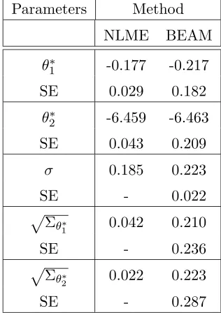
3.1 Results of estimation of parameters in the logistic growth model to the
data set on growth colonies of the bacteria Paramecium Aurelium using
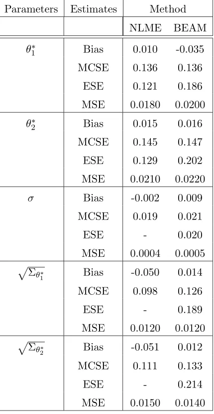
NLME and BEAM. . . 40 3.2 Simulation Results for the logistic growth model for colonies of
parame-cium aurelium (on log scale) using NLME and BEAM, with 500 MC Runs. 43
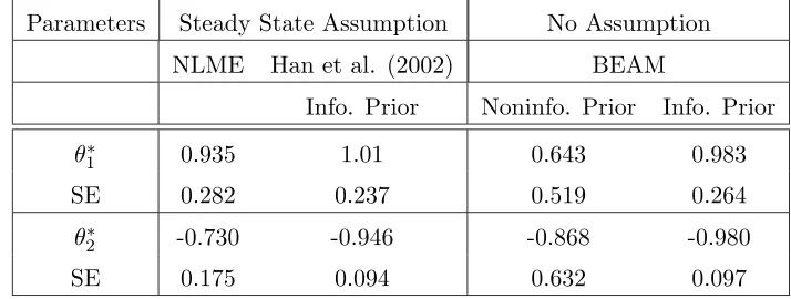
3.3 Results of estimation of parameters in the HIV model using BEAM, NLME and Bayesian hierarchical modeling involving a closed form expression for
the mean function. . . 47
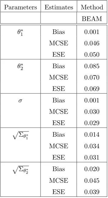
4.1 Simulation Results for HIV model using BEAM with 1000 MC Runs. . . 55
5.1 Results of estimation of parameters in the logistic growth model to the
data set on growth colonies of the bacteria Paramecium Aurelium using
2.1 Plots of observations on growth colonies of paramecium aurelium (in log
scale) and the estimated mean trajectories obtained by NLS, BEAM and
SEAM for each of the three data sets. . . 18 2.2 Box plots of point estimates: (i) ˆθ1’s (ii) ˆθ2’s (iii) ˆσ’s based on 1000
simu-lated data sets. (The horizontal solid line in each case represents the true
value of the parameters.) . . . 22
3.1 Plots of observations on growth colonies of paramecium aurelium (in log
scale) and the estimated mean trajectories obtained by NLME and BEAM
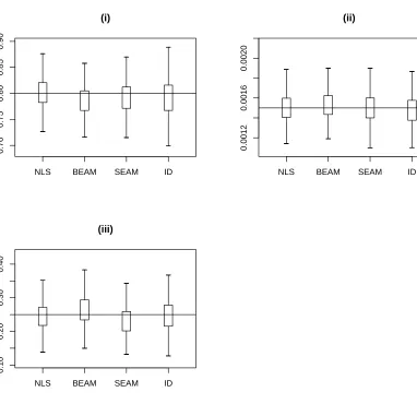
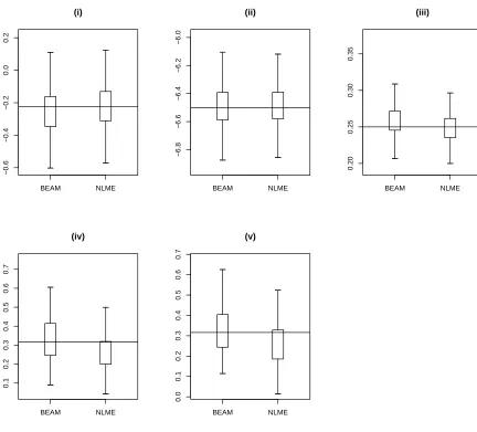
along with 95% posterior confidence band from BEAM. . . 41 3.2 Box plots of point estimates: (i) ˆθ∗
1’s (ii) ˆθ2∗’s (iii) ˆσ’s (iv)
q ˆ Σθ∗
1’s (v)
q ˆ Σθ∗
2’s based on 500 simulated data sets. (The horizontal solid line in
each case represents the true value of the parameters.) . . . 44
4.1 Box plots of point estimates: (i) ˆθ∗
1’s (ii) ˆθ2∗’s (iii) ˆσ’s (iv)
q ˆ Σθ∗
1’s (v)
q ˆ Σθ∗
2’s based on 1000 simulated data sets for HIV model. (The horizontal
Preface
Nonlinear mixed effects (NLME) framework is widely used in modeling repeated
mea-surements data, where meamea-surements are obtained for a number of individuals under
varying experimental conditions. Nonlinear mixed effects models incorporate population (fixed) as well as individual specific (random) characteristics and hence enable to make
inferences for both random and fixed effects. The concept of a nonlinear mixed effects
model was first introduced in Sheiner et al. (1972) to analyze the data pooled over all individuals and since then, there has been a great deal of further research (Davidian and
Giltinan, 1995) in population pharmacokinetics/pharmacodynamics (PK/PD) using
non-linear mixed effects models. Within the framework of nonnon-linear mixed effects (NLME) models, much of the interest is focused on representing the mean function (or mean
trajectory) describing the dynamic relationship between the response and explanatory
variables (such as time), by a system of ordinary differential equations (ODEs) whose
parameters describe the different characteristics of the underlying population. A system of ODEs provides an attractive modeling tool to describe a dynamic process, where the
interest is focused on modeling the rate of change over time rather than the static
av-erage value of the response variable, e.g., as in PK/PD models, viral dynamics etc. In real applications, it turns out that there are very few cases where it is actually possible
to derive the closed form expression for the exact solution, for a well-posed differential
equation problem. The absence of a closed form analytical solution for the system of ODEs makes parameter estimation in such models, challenging and computationally
de-manding. The objective of this research is to propose methodologies that approximate
the mean function and estimate the parameters involved in it, when an exact analytical form of the mean function is not available.
non-linear fixed effects models and compare the performance of these two methods Bayesian Euler’s Approximation Method (BEAM) and theSplines Euler’s Approximation Method
(SEAM) with other established methods in the literature by using a real data analysis
and a simulation study motivated by the real data analysis. In this case, the data sets
corresponding to several individuals/subjects were treated as separate data sets.
In Chapter 3, we extend the BEAM approach to the nonlinear mixed effects
frame-work, where population consists of several individuals and the individual specific
char-acteristics are incorporated within the model framework. A real data analysis and the corresponding simulation study were performed to compare the performance of BEAM
with an established approach in the literature (Lindstrom and Bates, 1990). We
imple-mented BEAMto a real data example where no closed form analytical solution exist for the system of ODEs, without assuming any assumption.
In Chapter 4, an additional simulation study was performed to illustrate the
appli-cation of BEAM to the multivariate data where data consists of (2× 1) observation vectors.
In Chapter 5, we summarized the results obtained in Chapters 2, 3 and 4 along with
Statistical Inference for Non-linear Fixed
Effects Models
2.1
Introduction
In the field of biomedical applications, data usually consists of repeated measurements
on individuals observed under varying experimental conditions. For example, in
phar-macokinetics, several blood samples are taken on participating individuals over a period of time, following the administration of a drug. These individuals can be considered as a
random sample drawn from a population of interest. More often, the relationship between
the measured response and the varying experimental conditions is nonlinear and involves unknown parameters of interest. The model is then fitted to data sets from different
in-dividuals, where the main interest is to make inferences about population characteristics
and in special cases, about individual characteristics which requires a mixed effects mod-eling framework. However, in this chapter we will treat the data set for each individual
as a separate data set and therefore the scope of this chapter is restricted to nonlinear
fixed effects models.
Within the the framework of nonlinear models (NLM), much of the interest is fo-cused on representing the mean function (or mean trajectory), describing the dynamic
relationship between the response and explanatory variables (such as time), by a
sys-tem of ordinary differential equations (ODEs) whose parameters describe the different characteristics of the underlying population. A system of ODEs provides an attractive
modeling tool to describe dynamic process, where the interest is focused on modeling the
ODEs and their results led to the conclusion that HIV virus has a high rate of replica-tion. In another example, a system of nonlinear ODEs was used to describe the temporal
expectation of virus and infected cell densities after initiation of anti-retroviral treatment
(Perelson et al., 1996). In the case of a HIV study, parameters involved in differential
equations, can characterize rates of production, infection, death of immune system cells and viral production and clearance (Ding and Wu, 1999).
It is well-known that when a closed form analytic solution is available for the system
of ODEs, the parameters can be estimated using standard statistical packages, e.g.,
R, SAS, WinBUGSetc. For example, in Han et al. (2002), parameters involved in a system
of ODEs were estimated using an analytical solution of the ODEs. The closed form
analytical solution was obtained by assuming that the virus dynamics are in steady state prior to the initiation of the anti-retroviral therapy. However, in practice it turns out
that such steady state assumptions may not hold and thus there are very few cases
where it is actually possible to derive the closed form expression for the exact solution for a well-posed system of ODEs. The parameter estimation problems for such models
become challenging and computationally demanding in the absence of any analytically
closed form solution for the system of ODEs.
The objective of this research is to develop computationally efficient methods to
obtain statistical inference for parameters of a NLM that involves a system of ODEs, in
the absence of an analytical solution. In Section 2.2, we describe the nonlinear statistical models and provide a brief review of the associated numerical methods. In Section 2.3, we
present the two proposed methods based on Euler’s approximation; (i) Bayesian Euler’s
approximation method (BEAM) in Section 2.3.1 and (ii) splines Euler’s approximation
method (SEAM) in Section 2.3.2. We then illustrate our methods in Section 2.4 by applying it to the data on growth colonies of paramecium aurelium. A simulation study
motivated by the previous application is then presented in Section 2.5. Finally, in Section
2.2
Nonlinear models involving ODEs
Let yj denote the jth observed response, measured at time point tj, for j = 1,2, ..., n
individuals. To keep our description simple, we considered time as the only dynamic
explanatory variable in the model. However, methodologies proposed in this chapter can be extended to a more general case with multiple dynamic covariates. The statistical
model can be written as,
yj =µ(tj,θ) +²j, j = 1,2, ..., n. (2.1)
In equation (2.1),µis the mean function describing the average dynamics of the response,
and depends on a vector θ= (θ1, . . . , θp)T of p regression parameters.
In the context of many biological applications (e.g., PK/PD or PBPK models), µcan
be defined as the solution of a system of ODEs given by
dν
dt = g(t,ν(t,θ)) for t6=t0 (2.2)
and ν(t0,θ) = ν0(θ) (2.3)
where ν(·) = (ν1(·), . . . , νq(·))T represents the underlying vector of dynamics and ν0(·)
provides a set of known initial conditions (often free ofθ). Theq-vector valued function
g(·) = (g1(·), . . . , gq(·))T that describes the dynamics is completely known up to the
unknown parameter θ. Notice that (2.2) can equivalently be expressed with a set of q
ODEs, dνk
dt =gk(t,ν(t,θ)) for k = 1, . . . , q.
The mean function, µ(·) is related to ν by a completely known function H: Rq →R
by µ(·) = H(ν(·)). In this chapter, for simplicity, we use single-compartmental system, i.e., q = 1, for all our illustrations but methods proposed in this chapter can be applied
to the general case of q ≥ 1 (Chapter 3). The random errors ²j’s correspond to the measurement uncertainties associated with the observed response at different time points.
zero mean and constant variance across all measurements, i.e.,
E(²j) = 0 and V ar(²j) =σ2, for j = 1,2, ..., n. (2.4)
The iidassumption for the errors is clearly restrictive and in Section 2.6 we discuss how
our methods can be extended to the case when we allow the variance of errors to change
with time, i.e., V ar(²j) = σ2(t
j,η) with unknown parameter η.
The objective is to estimate the parameter vector θ and the variance parameter, σ2.
The parameter estimates can be obtained by numerical methods, using packages likenlm
inRorproc nlininSASif an analytic closed form expression were available for the mean function µ(·). However, as we discussed earlier, in most cases, such an analytic solution for the system of ODEs either require restrictive assumptions or simply not available. The
lack of a closed form expression for the mean function makes the parameter estimation problem challenging and this is the focus of our research work.
The usual approach to overcome this problem, is to solve the system of ODEs
nu-merically by using popular ODE solvers at a known set of values of the parameter θ.
However the success of most of these numerical approximation methods depends on a “good” choice of a starting value for θ and some characteristics of the system (e.g., the
steepness etc.). A “bad” starting value often leads to an unstable solution and creates
numerical problems for the optimization method that is followed by these ODE solvers. The popular odesolve package in R provides an interface to the Fortran ODE solver
lsoda (Petzold, 1987). The numerical solution obtained from these ODE solvers are
then used to obtain parameter estimates either by a Bayesian method (Gelman et al., 1996; Wakefield, 1996; Lunn et al., 2002; Putter et al., 2002) or by the maximum
like-lihood method (Davidian and Giltinan, 1995; Racine-Poon and Wakefield, 1998). Even
though ODE solvers are widely used for estimating parameters in PK/PD modeling, it may be difficult to implement or lack control of essential numerical subroutines required
to obtain the desired numerical solution for ODE. Moreover these numerical methods also
iterative procedures in which the system of ODEs must be solved at each time point for each individual and this becomes more complicated in the case of multi-compartmental
problems with censored or missing data.
An alternative approach, known as the “Integrated Data (ID)” method for
parame-ter estimation for models described by a system of ODEs, was proposed by Holte et al. (2003). The idea behind the ID method is to simplify a nonlinear regression problem
by transforming a system of ODEs into a system of integral equations and fitting a
lin-ear regression model with “covariates” as the approximate integrals in these equations. However, the ID method requires a set of dense measurements taken from each
compart-ment represented in the ODE system, which may be difficult or costly, if not impossible,
especially when the system consists of multi-compartments.
In this chapter, we propose two alternative methodologies to resolve the numerical
problems related to parameter estimation for the situation when there is no closed form
solution available for the system of ODEs.
The first approach will be termed as the “Bayesian Euler’s Approximation Method
(BEAM)” which is built on the existing Bayesian framework for parameter estimation
in PK/PD modeling (Gelman et al., 1996; Lunn et al., 2002; Han et al., 2002; Putter et al., 2002; Wakefield, 1996; Huang et al., 2004) using the Euler’s method of solving
a system of ODEs and thus providing an analytic closed form approximation for the
likelihood function. The advantages of BEAM are in providing a closed form analytic approximation for the likelihood as well as its ability to handle missing or censored data
by using data augmentation methods (Schafer, 1997). It also has the flexibility to handle
sparse and/or unbalanced data. The availability of entire posterior distributions for the
unknown parameter (θ, σ) also makes it straightforward to draw statistical inferences. The second approach will be termed as the “Splines Euler’s Approximation Method
(SEAM)”, that uses a suitable class of interpolating spline functions (Wahba, 1990) to
pre-process the data before applying the Euler’s method to approximate the likelihood function. The advantages of SEAM are in relaxing the distributional assumptions for the
2.3
Likelihood approximation using the Euler’s method
Many different numerical approximation methods are available for computing
approxi-mate solutions to a system of ODEs with a given set of initial conditions such as the
generic problem given by (2.2) and (2.3).
According to the Lambert (1991), a numerical approximation method is basically a
prescription for replacing the system of ODEs by a system of linear algebraic equations
that can be solved on a computer using software written in a standard programming lan-guage. A detailed discussion of these methods can be found in the literature (Shampine,
1994; Lambert, 1991; Atkinson, 1978). All the numerical approximation methods involve
discretizing the time points by an amount h known as the “step size,” which is the dis-tance between two consecutive time points. This step size may or may not be the same
for all consecutive time points, but for our description we assume h to be constant over
the range of time points, i.e. we assume that t0
k = t0 +hk for k = 0,1,2, . . ., represent
the discretized time points. It is easy to see that the solution to the system of ODEs in
equation (2.2) can be expressed as
ν(t,θ) = Z t
t0
g(s,ν(s,θ))ds+ν0(θ) (2.5)
which suggests the approximation, as h→0,
ν(t+h,θ)−ν(t,θ) = Z t+h
t
g(s,ν(s,θ))ds ≈hg(t,ν(t,θ)) (2.6)
and hence an approximation for µ(t,θ) = H(ν(t,θ)), where H is a completely known
continuous function. Thus, using (2.6) we can obtain a recurrence relation to approxi-mate the mean function. We now describe a method based on (2.6) to approxiapproxi-mate the
likelihood that arise from the model given by equations (2.1-2.4). Let t1 < t2 <· · ·< tn denote the observed time points in the data set and we observe the response values
t0
k+1−t0k =h fork = 1,2, ...,(N−1). In order to cover the range of observed time points we choose the maximum value for these fixed time points to be larger than tn. In other
words, we assume t0
N > tn. The choice of h (and hence that of N) will depend on the sample size n. Letting ˜νk ≡ν˜(t0k,θ) and ˜µk ≡µ˜(t0k,θ) =H(˜νk) for k = 1,2, . . . , N −1, we can write
˜
νk+1 = ˜νk+hg(t0k,νk) ˜
µk = H(˜νk), (2.7)
with initial condition, ˜ν1 =ν0(θ). This simple approximation defined by equation (2.7),
forms the basis of our analytical approximation. Now to define ˜µ(t,θ) for any value of
t ∈[t0
1, t0N], we use a linear interpolation. More precisely, given a time point t ∈ [t01, t0N], we define the labels,
L(t) = N X
k=1
I(t0k ≤t). (2.8)
Notice that for anyt∈[t0
1, t0N], the functionL(t) takes the values in the range{1, . . . , N} and determines that how manyt0
k’s are less thant which in turn provides the lower limit of the interval that contains t, i.e., t0
L(t) ≤ t < t0L(t)+1. The value of approximate mean
function at t ∈[t0
1, t0N] is then given by,
˜
µ(t,θ)≡µ˜h(t,θ) = ˜µL(t)+
t−t0
L(t)
t0
L(t)+1−t0L(t)
(˜µL(t)+1−µ˜L(t)), (2.9)
whereL(t) is defined in (2.8) and ˜µk’s are defined in (2.7). Thus we can approximate the
true likelihood function of (θ, σ) using the ˜µ(t,θ) function. Notice that ˜µh(t,θ)→µ(t,θ) as h→0 (Lambert, 1991). In fact, ˜µh(t,θ) =µ(t,θ) +o(h) if we use the above method known as the “naive” Euler’s method. If we use the “improved” Euler’s method (see
Appendix A), then ˜µh(t,θ) = µ(t,θ) +o(h2) and more generally Runge-Kutta method
yields ˜µh(t,θ) = µ(t,θ) +o(h4). Thus, it follows that as h →0, the likelihood function
based on the approximating ˜µ(t,θ) function as defined above.
We now use (2.7) and (2.9) as the basis to propose two methods which can be further
improved using other numerical recipies as described in Appendix A at the cost of
com-putational time.
2.3.1
The Bayesian Euler’s Approximation Method (BEAM)
In order to construct a likelihood based on (2.9) we assume that the errors are iid
and normally distributed with mean zero and variance σ2. Given the observed data
D = {(Yj, tj) : j = 1,2, . . . , n} the model described by equations (2.1-2.4) can now be approximated by the following hierarchical model:
yj|(θ, σ2) indep
∼ N(˜µj(θ), σ2) for j = 1,2, ..., n (2.10)
where ˜µj(θ) = ˜µ(tj,θ) as defined in (2.9). For practical applications, theyj’s may be the log-transformed (or more generally Box-Cox transformed) values depending on whether
normality or log-normality is the more appropriate assumption for the data (Lunn et al.,
2002).
Second and the final stage of this hierarchical model consists of the specifying prior
distributions for parameters as follows:
θ|σ−2 ∼MVNp(θ0, H0) and σ−2 ∼G(a0, b0), (2.11)
where MVNp(θ0, H0) denotes a multivariate normal distribution with meanθ0 and
vari-ance matrixH0 and G(a0, b0) denotes a gamma distribution with meana0b0. The values
of a0, b0, θ0, H0, are assumed to be known, which are used to elicit prior information
when available. In the lack of prior information, we choose these known quantities to reflect on prior ignorance by choosing these values to yield vague priors (i.e., priors with
large variances). For a detailed discussion about the choice of prior distribution, see
based on the model (2.10-2.11) can be written as:
p(θ, σ−2|D)∝p(Y|θ, σ−2)p(θ)p(σ−2). (2.12)
where Y = (Y1, . . . , Yn). Clearly the above posterior density is analytically intractable
as it is highly nonlinear in θ. In order to use sampling based methods, such as Markov
chain Monte Carlo (Robert and Casella, 2005) we obtain the full conditionals of θ and
σ−2, which are given by,
p(θ|σ−2,D) ∝ p(Y|θ, σ−2)p(θ) (2.13) and p(σ−2|θ,D) ∝ p(Y|θ, σ−2)p(σ−2). (2.14)
If the right hand side of above equations have densities of the standard form then we
can use Gibbs sampling (Geman and Geman, 1984) to simulate values from the posterior distribution of (θ, σ−2). For instance a standard form is available for the full conditional
of σ−2:
σ−2|θ,D ∝G
a0+
n 2, Ã 1 b0 +1 2 n X j=1
(yj −µ˜j(θ))2 !−1
, (2.15)
and therefore we can easily draw samples from the full conditional ofσ−2. Since we do not
have a standard form for the conditional distribution of θ, we can use the
Metropolis-Hastings algorithm (Metropolis-Hastings, 1970) to draw samples. Though we used WinBUGS to generate approximate samples from posterior distribution of (θ, σ−2), here we give a
brief outline of the iterative MCMC algorithm suitable for BEAM.
1. Initialize the iteration of the chain at l = 0 and start with some initial values,
S(0) = (σ−2(0),θ(0))
2. Obtain S(l) fromS(l−1) in two steps:
(a) Draw σ−2(l) ∼π(σ−2|θ(l−1),Y) using (2.15) and
Evaluate the acceptance probability of the move, given by,
α(φ|θ(l−1)) = min
½
1, π(φ|σ−
2(l),Y)
π(θ(l−1)|σ−2(l),Y)
¾
Also, independently sample aufrom the uniform (0,1) and if u≤α(φ|θ(l−1)) the move is accepted else stay atθ(l−1).In other words, if the move is accepted then θ(l) =φ otherwise θ(l)=θ(l−1).
3. Move from chainltol+1 using step (2) and repeat until the Markov chain{S(l), l=
1,2, . . .} converges (to p(θ, σ−2|D)).
In practice,WinBUGSuses a Metropolis algorithm based on a normal proposal distribution
with the mean as the current value of the parameter and variance determined by tuning
over the first 4000 iterations to achieve an acceptance rate between 20% and 40%. In order to diagnose convergence of algorithms, we used graphical techniques such as history
plots (available inWinBUGS) of the values of the multiple chains for each parameter. Based
on these plots we decided upon an initial number of burn-in iterations (e.g., at least 4000) followed by say B = 2000 samples per chain drawn afterwards. We performed MCMC
sampling based on three parallel chains, therefore all the posterior summaries are based
on a total of 3B = 6000 samples. Mean of posterior distribution for each of unknown parameters was taken to be the posterior estimate of that unknown parameter along with
a 95% posterior interval formed by 2.5% and 97.5% posterior percentiles.
2.3.2
The Splines Euler’s Approximation Method (SEAM)
Interpolation is a method of constructing a smooth curve from a discrete set of known
data points, which is a specific case of curve fitting, in which the function must go
ex-actly through the data points. Spline interpolation is a form of interpolation where the interpolant is a special type of piecewise polynomial function called a spline. Spline
inter-polation is preferred over regular polynomial interinter-polation because the interinter-polation error
motiva-tion behind the second approach, “Splines Euler’s Approximamotiva-tion Method (SEAM)” is to obtain a smooth estimate of the mean using interpolating spline by regressing observed
response on observed time points. Given the observed data D (as defined in previous section), we fit a cubic spline interpolation passing through each of the time points tj’s.
More specifically for each interval [tj, tj+1], there is a separate cubic polynomial each with
its own coefficients:
Sj(t) =aj(t−tj)3+bj(t−tj)2+cj(t−tj) +dj for t∈[tj, tj+1]
together, these segments constitute the splineS(t) which must satisfy the following con-ditions:
(i) Piecewise continuous: Sj(tj) = yj, Sj(tj+1) =yj+1 and
(ii) First and second derivatives continuous: S0
j−1(tj) = Sj0(tj) and Sj00−1(tj) =
S00 j(tj).
A detailed discussion about splines and interpolation can be found in literature (Wahba,
1990).
In order to construct the approximating mean function ˜µ(t,θ), we use the following steps:
1. Fit an interpolating spline ˆY(t) by regressing observed data Yj’s on observed time
pointstj’s forj = 1,2, ..., nand obtain the predicted values ˆYk = ˆY(t0k), correspond-ing to each of the fixed time points t0
k = t0 +hk, for k = 1, . . . , N. This creates a
pseudo-data set {( ˆYk, t0k) :k = 1,2, . . . , N} suitable for Euler’s approximation. 2. Next, use Euler’s method (2.7) to construct an approximate mean function ˜µ(t0k,θ). 3. Finally, obtain the least square estimate ˆθ by minimizing
SS(θ) = N X
k=1
( ˆYk−µ˜(t0k,θ))2, (2.16)
and then obtain ˆσ2 = 1
N−p PN
The first advantage of this approach lies in the fact that no parametric distribution as-sumption is necessary for the errors. Another advantage comes from the use of splines
for curve fitting, since splines can be used to fit data observed over sparsely and unevenly
spaced time points, the SS(θ) defined by (2.16) becomes a smooth function of θ
facili-tating the minimization problem in (2.16). Moreover, this approach is computationally very efficient and easy to implement requiring no iterative procedure. Therefore, SEAM
provides an attractive tool in comparison of other computationally intensive procedures.
2.4
Analysis of Growth Colonies of
Paramecium
Au-relium
Diggle (1990) presents a data set that describes the growth of three closed colonies
of paramecium aurelium in a nutritive medium on a 19 days period. For a detailed
description of this experiment, we encourage readers to refer to Diggle (1990, p. 8). One
of the main goals of this experiment was to develop a dynamic model for the growth count (say xj’s) of paramecium aurelium, as a function of time t. The data is assumed
to follow a log-normal distribution, with
yj = log{xj} = log{ν(tj,θ)}+²j
= µ(tj,θ) +²j, ²j ∼N(0, σ2) (2.17)
wherexj is the observed growth count at time point tj (measured in days) andµ(tj,θ) = log{ν(tj,θ)}.
Next, it is assumed that ν(t) follows the standard 2 parameter logistic growth curve
described by the non-linear differential equation
dν
dt = g(t, ν(t,θ))
Equivalently, we can express the equation(2.18) in terms ofµ(·):
dµ
dt = g
∗(t, µ(t,θ)))
≡ θ1 −θ2eµ and µ(0) = log(2). (2.19)
In a logistic growth curve model,θ1 represents the growth per capita, θ1/θ2 measures the
carrying capacity of the population, and y0 represents the initial size of the population.
There are three data sets consisting of individual counts, corresponding to three
replications of the same experiment and here we analyzed all three data sets separately. Although we proposed our estimation methods for situations where an analytical closed
form solution is not available for the system of differential equations, here an analytically
closed form solution is actually available. The reason behind the choice of this simple growth curve model is that it will allow us to compare the performance of the
estima-tion based on our proposed approaches to that based on the ideal nonlinear regression
approach, which requires a closed form mean function be available. A detailed descrip-tion of nonlinear regression techniques can be found in a classic book by Davidian and
Giltinan (1995). We will also perform ID method (Holte et al., 2003) on these three data
sets.
To approximate the likelihood using BEAM, we chose N = 19 and for SEAM we
choseN = 40. These choices of the tuning parameter N (or equivalently, h= t0N−t
0 1
N ) are not based on any analytical work, rather the choices are mainly driven by computational convenience. In general, the finer the grid points (with large N and hence small h) is
chosen, the better the likelihood will be approximated. Alternatively, one may also use
improved numerical approximation methods (such as those described in the Appendix A) at the cost of computing time.
To implement the BEAM on this log transformed data, we followed the same steps
as described in Section 2.3.1, coupled with equations (2.17) and (2.19). For the MCMC
chain, giving us a total of 6000 approximate samples from the posterior distribution of (θ, σ), where samples for σ were observed by calculating σ = √1
σ−2. Convergence of
the chains was diagnosed visually by inspecting simultaneous trace and acf plots of the
values of all three chains, for each parameter. Plots showing a good mixing of chains
were a reasonable indication for convergence. The software WinBUGS freely available at the website http://www.mrc-bsu.cam.ac.uk/bugs/ was used to perform all of the
computations for this data analysis. The following values were used to elicit priors:
θ0 = (0,0)T, H
0 = 10I2×2 for the prior on θ and a0 = b0 = 0.01 for the prior on
σ−2. Finally, the MC estimate of the mean and standard deviation of the posterior
distributions for these parameters were used as point estimates and standard errors,
respectively.
In a similar approach, to implement SEAM to fit the model to these data sets we
followed the same steps as described in Section 2.3.2. The function “interpSpline” in
R was used to obtain the spline interpolation followed by the use of the optim function available inR to perform the minimization ofSS(θ) function in (2.16). Finally, to fit the
NLM, we usednlm function in R to obtain parameter estimates and associated standard
errors (SE).
Results from all four estimation approaches are presented in Table 2.1. In Table
2.1, we presented estimates and standard errors for parameters θ = (θ1, θ2) and σ,
cor-responding to nonlinear least square (NLS) method, BEAM, SEAM and ID method. Estimated standard errors for the parameterσ are not presented in the table, because of
its unavailability with the statistical software used to minimize the likelihood functions in
“NLS”, “SEAM” and “ID” methods. Additionally, in order to compare the performance
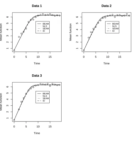
of these estimation approaches, we plotted estimated mean function corresponding to four approaches along with the observed data points in Figure 2.1. From Figure 2.1,
all four approaches seem to perform very similarly in capturing the trajectory of mean
function reasonably well. It can also be observed from Figure 2.1 that both BEAM and SEAM provide data fits close to the fits obtained by using the NLS method, which uses
Table 2.1: Parameter estimates and standard errors (SE) based on the logistic growth model for colonies of the bacteria paramecium aurelium using NLS, BEAM and SEAM methods to fit three data sets.
Data Set Estimates Method
NLS BEAM SEAM ID
I θˆ1 0.789 0.760 0.783 0.767
ESE 0.025 0.029 0.044 0.015
ˆ
θ2(∗10−3) 1.446 1.470 1.464 1.369
ESE 0.120 0.152 0.238 0.055
ˆ
σ 0.218 0.266 0.233 0.187
ESE - 0.049 -
-II θˆ1 0.837 0.803 0.827 0.792
ESE 0.025 0.034 0.049 0.015
ˆ
θ2(∗10−3) 1.672 1.678 1.685 1.548
ESE 0.126 0.175 0.265 0.057
ˆ
σ 0.201 0.266 0.207 0.164
ESE - 0.049 -
-III θˆ1 0.892 0.857 0.875 0.856
ESE 0.018 0.025 0.051 0.011
ˆ
θ2(∗10−3) 1.594 1.596 1.579 1.489
ESE 0.078 0.118 0.246 0.063
ˆ
σ 0.132 0.201 0.137 0.135
-0 5 10 15 1 2 3 4 5 6 Data 1 Time Mean function BEAM NLS SEAM ID
0 5 10 15
1 2 3 4 5 6 Data 2 Time Mean function BEAM NLS SEAM ID
0 5 10 15
1 2 3 4 5 6 Data 3 Time Mean function BEAM NLS SEAM ID
estimated standard errors (ESE) for parameters θ1 and θ2 are smaller for ID method
than remaining other three approaches which may appear to suggest that ID method
provides more precise estimates than other approaches. However this situation seems
to arise from the estimation approach for σ by ID method. ID method estimates the
population variance beforehand and then plugs in that estimated variance in the model. This estimated variance is then treated as a known parameter while estimating rest of
the parameters in the model. Here an estimate is being considered as a known value for
rest of the estimation procedure and therefore uncertainty associated with this estimate is not being accounted. Therefore, this plug-in variance estimator leads to the
underes-timation of variance of θ1 and θ2 both. Mathematically, estimated variance of ˆθi can be expressed as
V(ˆθi) =E[V(ˆθi|σˆ)] +V[E(ˆθi|ˆσ)], i= 1,2 (2.20) Now under the ID method, since ˆσ is treated as known while estimating θ, the second term on the right hand side of equation (2.20) becomes zero. This leads to the
under-estimation of V(ˆθi) for i = 1,2. It can be noticed in next section that the simulation
standard error for parameters, in Table 2.2 are in accordance for all four methods. We also used BEAM to calculate the point estimates based on the posterior distribution of
the carrying capacity per capita (θ1/θ2) for all three data sets, along with the
correspond-ing 95% posterior credible interval. These point estimates were obtained by calculatcorrespond-ing the mean of ratio of posterior samples for θ1 and θ2. For the data set (1), the
esti-mated carrying capacity is 523.91 and the corresponding 95% posterior credible interval
is (445.80, 606.92). For the data set (2), the estimated carrying capacity is 526.88 and the corresponding 95% posterior credible interval is (448.19, 612.83). Similarly, for the data
set (3), the estimated carrying capacity is 533.74 and the corresponding 95% posterior
2.5
Simulation Study
A simulation study, motivated by the above real data analysis was carried out to compare
the performance of the two proposed methods, BEAM and SEAM, to the NLS procedure,
in terms of estimation accuracy and efficiency. The true values of parameters for data generation are chosen based on the estimates obtained for the real data application. For
the simulation study, data is generated using the model (2.19) with µ(t,θ) given by the
closed form solution:
µ(t,θ) = log(ν(t,θ))
= log(θ1) +µ(0) +tθ1−log[θ2eµ(0)(etθ1 −1) +θ1] (2.21)
We chose the time points as given in the real data set and simulated data sets using
equation (2.17) and (2.21) with true values of the parameter set atθ1 = 0.8,θ2 = 0.0015
and σ = 0.25.
We chose the sample size same as the real data set, i.e., n = 19 and replicated the
data generations for 1000 Monte Carlo runs. To fit the model by BEAM we choseN =n
and the same prior distribution as used in the real data analysis and used same number of burn-in and MCMC samples for each of the 1000 data sets as was used in the real
data application. Similarly for SEAM we used N = 40 to fit the models to each of the
simulated data sets.
A summarization of the comparative study of the four procedures based on this simu-lation study are given in Table 2.2 and Figure 2.2. In Table 2.2, we summarize our finding
in terms of (i) the bias, which is the difference between the MC mean of the point
esti-mates and the true value of a parameter; (ii) the estimated standard error (ESE), which is the MC mean of the standard errors of the parameter estimates, (iii) the Monte Carlo
simulation standard error (MCSE), which is the standard deviation of the estimates and
(iv) the mean square error (MSE) obtained as Bias2+ MCSE2.
From Table 2.2, it is evident that all four methods performed equally well in terms of
Table 2.2: Simulation Results for the logistic growth model for colonies of paramecium aurelium using NLS, BEAM, SEAM and ID Methods with 1000 MC Runs.
Parameters Estimates Method
NLS BEAM SEAM ID
θ1 Bias 0.002 -0.014 -0.008 -0.007
MCSE 0.029 0.028 0.029 0.035
ESE 0.029 0.029 0.233 0.017
MSE 0.001 0.001 0.001 0.001
θ2(∗10−3) Bias 0.005 0.036 0.017 -0.024
MCSE 0.146 0.149 0.149 0.152
ESE 0.140 0.152 0.235 0.063
MSE 0.021 0.024 0.022 0.024
σ Bias -0.005 0.014 -0.017 -0.002
MCSE 0.042 0.044 0.044 0.045
ESE - 0.048 -
-MSE 0.0018 0.0021 0.0022 0.0021
parameter estimates in comparing the BEAM and SEAM with the NLS and ID method,
we present box plots of the estimates obtained by each of the four methods in Figure 2.2.
The horizontal solid line in each case represents the true value of the parameter. Figure 2.2 reveals that although BEAM and SEAM tend to underestimateθ1, the inter-quartile
range of the estimates from all four methods contain the true value of θ1. Similarly for
θ2, we observe from Figure 2.2 and Table 2.2 that in this case as well, all four methods
perform almost identically. For σ, Figure 2.2 apparently indicates that BEAM tends to
overestimate and SEAM tends to underestimate the true value but none of these biases are
statistically significant. Finally, in terms of comparing the MSEs (see Table 2.2) obtained by these four methods, we find that, as expected NLS has the minimum MSE compared
to the two proposed methods and ID method, but the gain is very nominal considering
NLS BEAM SEAM ID
0.70
0.75
0.80
0.85
0.90
(i)
NLS BEAM SEAM ID
0.0012
0.0016
0.0020
(ii)
NLS BEAM SEAM ID
0.10
0.20
0.30
0.40
(iii)
Figure 2.2: Box plots of point estimates: (i) ˆθ1’s (ii) ˆθ2’s (iii) ˆσ’s based on 1000 simulated data
an analytically closed form for the mean function is not available, NLS is not applicable, but BEAM and SEAM will still work.
2.6
Discussion
The main objective of the data analysis (in Section 2.4) and simulation study (in Section
4) was to compare the performance of BEAM and SEAM with NLS for situations where a closed form analytical solution for system of differential equations is available. Results
of data analysis and simulation study suggest that both of these methods provide results
very close to the results obtained by the NLS method and therefore the Euler’s approxi-mation to the mean function described in Section (2.4) works quite accurately. Also the
strikingly similar values of the MSE’s of the parameters suggest that the proposed
meth-ods are as efficient as the NLS method when an analytic solution is available. Though for the model considered in this chapter, ID method also provided similar results, it
re-quires certain assumptions to be satisfied. For example, this method rere-quires that the
maximum interval length between two consecutive time points should be O(n−1), which
may or may not be true, specially for large longitudinal studies.
In this chapter we assumed that random errors are identically, independently
dis-tributed but methodologies presented here are not restricted to this assumption. This
assumption can be relaxed by using a generalized nonlinear modeling framework (David-ian and Giltinan, 1995) with ˜µ(t,θ) as the mean function and σ2(t,η) as the variance
function, which is assumed to be a known function up to the unknown parameter η. In
order to implement BEAM with this generalized nonlinear modeling framework we need to use suitable priors for the parameter η of the variance function. For the SEAM we
have to replace the SS(θ) in (2.16) by a weighted least square criteria, where say the
weights can be chosen to be inversely proportional to the variance function.
Further, in most of biomedical applications, data constitutes of several individuals
and modeling of such data involves population specific parameters as well as
for this research consists of extending the proposed methodologies to the mixed effects model framework where data are subject to missingness and censoring.
One of the main advantages of BEAM and SEAM is that these do not require any
restrictive assumptions other than those typically considered in nonlinear modeling. The
proposed likelihood approximation method also provides a closed form approximation of the mean function, ˜µ(t,θ). Therefore these methods can be used to estimate the mean
function at any time point lying within the close vicinity of the observed time range. This
is a huge advantage as it avoids evaluating the numerical solution of the mean function at the parameter estimate again and again for interpolation/extrapolation. Because of
the Bayesian framework, one of the key advantages of BEAM also lies in its ability to
handle missing data that is very common in longitudinal studies. The availability of posterior distributions for the unknown parameters, also makes it straightforward to
draw statistical inferences. At the same time advantage of SEAM comes from not only
from its accuracy of estimation and weaker distributional assumptions but also from its computational convenience as compared to BEAM. Although BEAM provides estimates
that are not only accurate but applicable with missing or censored data, there is no
denying that this is a computationally intensive procedure. In comparison to BEAM, SEAM takes much less computation time, but SEAM is limited to handling only
un-censored data. At the end, we will leave the choice between BEAM and SEAM up to
readers, as both have their pros and cons.
For our proposed methods, we used the “naive” Euler’s approximation method in
both cases. We chose Euler’s approach just for the sake of simplicity and also because it
provided reasonable estimates for parameters in our simulation studies. However, other
Bayesian Inference in Non-linear Mixed
Effect Models involving ODEs
3.1
Introduction
Nonlinear mixed effects (NLME) models are widely used in practice involving data sets,
where repeated measurements are obtained for a number of individuals under varying
experimental conditions. Nonlinear mixed effects models incorporate population level (fixed) effects as well as individual specific (random) characteristics and hence enable
to make inferences for both random and fixed effects. The conceptual framework of a
nonlinear mixed effects model was first introduced by Sheiner et al. (1972) to analyze the data pooled over all individuals and since then, there has been an explosion of
fur-ther research (Davidian and Giltinan, 1995) with application to population
pharmacoki-netics/pharmacodynamics (PK/PD) models and physiologically based pharmacokinetic (PBPK) models based on nonlinear mixed effects modeling framework. Within the
frame-work of NLME models, much of the interest is focused on representing the mean function
(or mean trajectory), describing the dynamic relationship between the response and
ex-planatory variables (such as time), by a system of ordinary differential equations (ODEs) whose parameters describe the different characteristics of the underlying population. A
system of ODEs provides an attractive modeling tool to describe dynamic processes,
where the interest is focused on modeling the rate of change over time rather than the static average value of the response variable, e.g., as in PK/PD models, viral dynamics
etc. As an illustrative example, consider a very commonly used system of differential
anti-retroviral treatment given by:
dν1
dt = −δν1+kT0ν2, ν1(0) =T
∗
0,
dν2
dt = −cν2, ν2(0) =VI0, (3.1)
dν3
dt = Nf vδν1−cν3, ν3(0) =VN I0.
In this model, ν1(t), ν2(t) and ν3(t) represent the density of infected cells at time t,
the density of infectious virus at time t and the density of non-infectious virus at time
t respectively. k is the infectivity constant, T0 is the density of un-infected cells at
the initiation of treatment, δ is the death rate for infected cells, c is the clearance rate
for free virus, and Nf v is the number of free virions produced per infected cell in its lifetime. T∗
0, VI0, andVN I0 are the known initial values (att=0) forν1(t),ν2(t) andν3(t)
respectively. If unknown, these initial values can be treated as parameters in the model
and can be estimated along with other parameters involved in the model. Assuming that
the virus dynamics are in quasi-steady state prior to the initiation of the treatment i.e.,
Nf vkT0 = c, Perelson et al. (1996) solved this system of ODEs for total viral density
V(t) = ν2(t) +ν3(t) at time t and the solution is given by
V(t) =V0exp(−ct) +
cV0
c−δ
·
c
c−δ{exp(−δt)−exp(−ct)} −δtexp(−ct)
¸
, (3.2)
where V0 =VI0 +VN I0. However, in practice it turns out that this steady state
assump-tion usually holds only during a short period after the initiaassump-tion of treatment (Wu, 2005)
and thus there are very few cases where it is actually possible to derive the closed form
expression for the exact solution for a well-posed differential equation problem. The absence of a closed form analytical solution for the system of ODEs makes parameter
estimation in such models, challenging and computationally demanding.
In this chapter, we aim to extend the Bayesian Euler’s approximation method (BEAM)
proposed in the previous chapter, to the nonlinear mixed effects framework involving a
describe a statistical framework for nonlinear mixed effects models followed by the de-scription ofBEAMfor mixed effects models in Section 3.3. We then illustrate the method
in Section 3.4 by applying it to a data on growth colonies of paramecium aurelium and
a simulation study motivated by the real data analysis is then presented in Section 3.5,
followed by the application of BEAM to the motivating example described by equation (1), in Section 3.6. Finally, in Section 3.7, we provide some general conclusions and
directions for future research.
3.2
Nonlinear mixed effects models involving ODEs
The problem in hand can be described as follows. Let yij denotes the jth observed
response, for the ith individual measured at timepoint tij, for i = 1,2, ..., m and
j = 1,2, ..., ni. For example, in the pharmacokinetic settings, tij can be the time associated with thejth drug concentration for subjecti. To keep our description simple,
we considered time as the only dynamic explanatory variable in the model. However,
methodologies proposed in this chapter can be extended to a more general case with
multiple dynamic covariates. A statistical model can be written as,
yij =µ(tij,θi) +²ij, for i= 1,2, . . . m and j = 1,2, ..., ni (3.3)
In equation (3.3),µis the mean function describing the within-individual behavior, which
depends on a vector ofp parameters,θi, specific to individuali. The random effectsθi’s are assumed to arise from a common distribution with mean θ and variance Σθ. More
specifically we can write
θi =θ+ei; E(ei) =0, V(ei) = Σθ (3.4)
sub-vector of remaining unknown individual specific parameters. For an individual i, the intra-individual error²ij corresponds to the measurement uncertainty associated with the
observed response at time pointtij. These random errors are assumed to be independently
distributed with zero mean and constant variance across all measurements, i.e.,
E(²ij) = 0 and V ar(²ij) = σ2 for i= 1,2, ..., m and j = 1,2, ..., ni (3.5)
For simplicity, errors are assumed to be iid though this assumption is clearly restrictive.
However, the method described in this chapter can be extended to the case when we allow
variance of errors to be of the form,V(²i) = σ2D
i whereDi is a ni×ni positive definite matrix, that may or may not depend on additional parameters and²i = (²i1, ²i2, ..., ²ini)
T .
We will discuss this aspect briefly in Section 3.7. Further ei and ²i are assumed to
be independent. Then the likelihood function for this modeling framework assuming normality of the responses and random effects can be written as ,
L(θ,Σθ, σ)∝
m Y
i=1
Z ni
Y
j=1
1
σe
− 1
2σ2(yij−µ(tij,θi)) 2
|Σθ|−1/2e−12(θi−θ)
TΣ−1
θ (θi−θ)dθ
i = m Y i=1 µ 1 σ2
¶ni2
|Σθ|−1/2
Z
e
− 1 2σ2
ni
X
j=1
(yij −µ(tij,θi))2− 1
2(θi −θ) TΣ−1
θ (θi−θ)
dθi (3.6)
Ideally, the parameters involved in the NLME model can be estimated by maximizing
the likelihood function, given by equation (3.6). If µ is a linear function in terms of parameters θi, the intergral in equation (3.6) can be evaluated to obtain an analytic
expression. However, more often in case of NLME models, µ is a nonlinear function
of parameters θi, making it impossible to obtain an analytic expression for the integral described in equation (3.6) and therefore classical approach such as maximum likelihood
method for parameter estimation becomes analytically intractable. A common approach
to handle the integral (with respect toθi) in (3.6) involves linearization of the nonlinear model by using either Taylor’s series expansion (Beal and Sheiner, 1982; Lindstrom and
and then estimating parameters from the resulting approximated likelihood functions. A detailed description of these procedures is presented in Davidian and Giltinan (1990,
p.151). A common feature of these approximation procedures is the availability of a
closed form expression for the mean function µ(·,θ). In the context of many biological applications (e.g., PK/PD models) µ is obtained as the solution to a system of ODEs given by,
d(ν(t,θ))
dt = g(t,ν(t,θ)) ∀θand t6=t0 (3.7)
and ν(t0,θ) = ν0(θ) (3.8)
where ν(·) = (ν1(·), . . . , νq(·))T represents the underlying vector of dynamics and ν0(·)
provides a set of known initial conditions (often free ofθ). Theq-vector valued function g(·) = (g1(·), . . . , gq(·))T that describes the dynamics, is completely known up to the
unknown parameter θ. Notice that (3.7) can equivalently be expressed with a set of q
ODEs, dνk
dt =gk(t,ν(t,θ)) for k = 1, . . . , q. The mean function, µ(·) is related to ν by a completely known functionH: Rq →Rbyµ(·) =H(ν(·)). For instance, in the case of the model described by equation (3.1), the mean functionµ(t,θi) =log(ν2(t,θi) +ν3(t,θi)).
In the absence of a closed form solution to the system described by equation (3.7), the usual approach to overcome this problem, is to solve the system of ODEs numerically
by using popular ODE solvers at a given set of values of the random effects θi’s and
use those numerical solutions in the estimation procedure (Davidian and Giltinan, 1995). These numerical solutions obtained from the ODE solvers can also be used in nonlinear
hierarchical Bayesian framework (Gelman et al., 1996; Wakefield, 1996; Lunn et al., 2002;
Putter et al., 2002), to estimate the parameters involved in the model. The Fortran ODE solver lsoda (Petzold, 1987) and the odesolve package in R that provides an interface
to the Fortran ODE solver are commonly used for this purpose. However, the success
of most of these numerical approximation methods depends on a “good” choice of a
for the optimization method that is followed by these ODE solvers.
Even though ODE solvers are widely used for estimating parameters in PK/PD
mod-eling, it may be difficult to implement or lack control of essential numerical subroutines
required to obtain the desired numerical solution for ODE and sometimes also turn out
to be unstable especially in case of censored or missing data (Putter et al., 2002). Apart from such numerical instabilities, these methods are computationally intensive iterative
procedure in which the system of ODEs must be solved at each time point for each
individual and this becomes more complicated in the case of multi-compartmental prob-lems with censored or missing data. For situations where the use of ODE solvers is
combined with approximated likelihood using Taylor’s series expansion (Lindstrom and
Bates, 1990) or using Laplace’s approximation (Wolfinger, 1993), the system of ODEs as well as the derivatives of the mean function (obtained by solving the system of differential
equations), need to be evaluated for all random effects parameters, at each time point.
The extent of computational burden increases with the increase in number of random effects parameters.
The objective of this research is to estimate the parameters involved in the NLME
model (3.3-3.5) by providing a closed form approximation to the mean function described by the system of ordinary differential equations. In this research, we are mainly interested
in the estimates of the “mean” of the random effects (θ), intra-individual variability (σ2)
and the variability associated with the random effects (Σθ).
In this chapter, we extend the Bayesian Euler’s approximation method (BEAM),
ear-lier proposed for nonlinear fixed effects models (Chapter 2), to the nonlinear mixed effect
framework. This approach combines the existing Bayesian framework for parameter
es-timation in PK/PD modeling (Gelman et al., 1996; Lunn et al., 2002; Han et al., 2002; Putter et al., 2002; Wakefield, 1996; Huang et al., 2004) with a numerical approximation
method, providing an analytical closed form approximation for the system of ordinary
differential equations. The advantages of this method lies in providing a closed form approximation for the solution of system of ordinary differential equations thus removing
equa-tions for every random effects parameter separately. This is a great advantage because not only this saves a lot of computational difficulty but also the approximated mean
function can be incorporated in nonlinear Bayesian hierarchical modeling to obtain
pa-rameter estimates, without imposing any restrictive condition about the mean function.
Due to its Bayesian framework this approach has the ability to handle the missing data by using data augmentation methods (Schafer, 1997) and the flexibility to handle sparse
and unbalanced data by utilizing information across individuals sampled from the
pop-ulation. The availability of posterior distributions for the unknown parameters involved in the model, also makes it straightforward to draw statistical inferences. This method
involves a numerical approximation method, viz. naive Euler’s approximation method
that provides reasonably good results in this case but there are more accurate numerical approximation methods, which can be used in place of Euler’s method, without any loss
of generality.
3.3
The Bayesian Euler’s Approximation Method
Many different numerical approximation methods are available for computing approxi-mate solutions to system of ODEs with a given initial condition such as the problem
given by (3.7) and a detailed discussion of these methods can be found in the literature
(Shampine, 1994; Lambert, 1991; Atkinson, 1978). The algorithm for BEAM is based on the Euler’s approximation method. All the numerical approximation methods involve
discretizing the time points by an amount h known as the “step size,” which is the
dis-tance between two consecutive time points. This step size may or may not be same for all consecutive time points, but for our description we assume h to be constant over the
range of time points, i.e., we assume that tk = t0 +kh for k = 0,1,2, .... Mostly, a
uniform step size is used to simplify programming. It is easy to see that the solution to the system of ODEs given by equation (3.7) can be expressed as
ν(t,θ) = Z t
t0
which suggests the approximation, as h→0,
ν(t+h,θ)−ν(t,θ) = Z t+h
t
g(s,ν(s,θ))ds ≈hg(t,ν(t,θ)) (3.10)
and hence an approximation for µ(t,θ) = H(ν(t,θ)) for all values of the parameter θ, whereH is a completely known continuous function. Thus, using (3.10) we can obtain a
recurrence relation to approximate the mean function.
We now describe a method based on (3.10) to approximate the likelihood that arise from the model given by equations (3.3-3.7) and the observed data D ={(Yij, tij) : i= 1,2, . . . , m and j = 1,2, . . . , ni}. Here ti1 < ti2 < · · · < tini, denote the observed time
points for the ith individual in the data set and {Y
ij = Y(tij) : i = 1,2, . . . , mand j =
1,2, . . . , ni} denote the response values. As the observed time points can be unevenly distributed we first consider a discretization byN fixed time points t0 =t01 < t02 < ... < t0N such thatt0
k+1−t0k =hfork = 1,2, ...,(N−1). In order to cover the range of observed time points we choose the maximum value for these fixed time points such thatt0
N ≥ max
1≤i≤mtini. The choice of N (and hence that of h) will depend on ni. Letting ˜νk(θ)≡ ν˜(t0k,θ) and ˜
µk(θ)≡µ˜(t0
k,θ) = H( ˜νk(θ)) for k= 1,2, . . . , N −1, we can write ˜
νk+1(θ) = ˜νk(θ) +hg(t0k,νk(θ)) (3.11) ˜
µk(θ) = H(˜νk(θ)) (3.12)
with initial conditions ˜ν1(θ) = ν0(θ). This simple approximation defined by equations (3.11) and (3.12) is known as the naive Euler’s approximation and forms the basis for most
of the numerical approximation methods available in the literature. A brief description
of some refined and numerically more accurate approximation methods that are used in practice is given in Appendix A. We now use (3.11) as the basis to a method which can
be further improved using other numerical recipies at the cost of computational time.
Now to define ˜µ(t,θi) for any value of t ∈ [t0