!
"
#"#
$ % %#
&
'
((( )
Multicategory Classification Using Relevance Vector Machine for Microarray Gene
Expression Cancer Diagnosis
Dr. S. Santhosh Baboo
Reader, PG and Research department of Computer Science, Dwaraka Doss Goverdhan Doss Vaishnav College
Chennai, Tamil Nadu,INDIA. [email protected]
Mrs. S. Sasikala*
Research Scholar, Dravidian University, AndraPradesh Head, Department of Computer Science Sree Saraswathi Thyagaraja College, Pollachi,
Coimbatore, Tamil Nadu, India. [email protected]
Abstract— This paper deals with the advancement in cancer multicategory classification using Relevance Vector Machine (RVM) for microarray gene expression cancer diagnosis. The proposed technique can be highly used for directing multicategory classification problems in the cancer diagnosis area. SVM and ELM are the presently available techniques used for binary classification tasks, which is related to and contains elements of non-parametric applied statistics, neural networks and machine learning. The cancer classification using the present approach does not provide the expected accuracy and sometimes the result of clustering may be wrong. To overcome this problem an efficient cancer classification using the Relevance Vector Machine (RVM) is proposed in this paper. This learning algorithm can generate accurate and robust classification results on a sound theoretical basis, even when input data are non-monotone and non-linearly separable. The performance of RVM is evaluated for the multicategory classification on two benchmark microarray data sets for cancer diagnosis, namely, the Lymphoma and Leukemia dataset. The results indicate that RVM produces better classification accuracies than the approach using SVM and ELM when the data given as input are preprocessed. RVM delivers very high performance with reduced training time and implementation complexity is less when compared to artificial neural networks methods like conventional back-propagation ANN and Linder’s SANN.
Keyword- RVM, SVM, ELM, ANOVA, Cancer Classification and Gene Expression
I. INTRODUCTION
Cancer is one of the dangerous diseases found in most of the living organism, which is one of the challenging studies for scientist towards 20th century. There were lot of proposal from various pioneers and detailed picture study was still going on. BasicallyCancer is characterized by an abnormal, uncontrolled growth that may destroy and invade adjacent healthy body tissues or elsewhere in the body. Living organisms such as animals and plants are made of cells. The simplest organisms consist of just a single cell. The human body compromises of billions of cells; most of the cells have a limited life-span and need to be replaced cyclic manner. Each cell is capable of duplicating themselves. Millions of cell divisions and replications take place daily in the body and it is astounding that the process occurs so perfectly most of the time every cell division requires replication of the 40 volumes of genetic coding. On rare circumstances there is some defect in a division and a rogue, potentially malignant cell arises. The immune system seems to recognize such occurrences and is generally capable of removing the abnormal cells before they have an opportunity to proliferate. Rarely, there is a failure of the mechanism and a potentially malignant cell survives, replicates and cancer is the result.
The activities of several thousand genes are simultaneously computed by High-density DNA microarray and the gene expression profiles have been used for the cancer classification recently. Although traditional linear techniques like principal component analysis (PCA), Fisher’s linear discriminant (FLD) etc., have been used for
this purpose; use of sophisticated, state-of-the-art techniques is receiving increasing attention for their superior performance. These include artificial neural network (ANN), wavelet transforms [32], maximum representation and discrimination feature (MRDF) [33], and more recently support vector machine (SVM). SVM is best suited for this kind of supervised classification problems among the above mentioned classifiers [31]. The fundamental idea of SVM is to map a set of input data to a high-dimensional feature space through a kernel function and separate classes in the kernel induced feature space with a maximum margin hyperplane that maximizes the minimum distance from the hyperplane to the closest input data points. In general, the hyperplane corresponds to a non-linear decision boundary in the input space and depends only on a subset of the original input data called the support vectors. The development of the technique relies on the theory of uniform convergence in probability and associated structural risk minimization (SRM) principle [35]. Palmer et al. [24] have used a linear SVM classifier for classifying in vitro autofluorescence and diffuse reflectance spectra of breast tissues and reported excellent classification results. Lin et al. [34] have used SVM to classify nasopharingeal tissues based on features extracted using linear PCA of in vivo autofluorescence spectra from nasopharingeal tissues and demonstrated significantly improved classification performance of combined SVMPCA algorithm as compared to that based on linear PCA alone.
probability of classification of the tissue to different classes. Such classification is particularly important in the context of
asymmetric misclassification costs where the
misclassification cost associated with some classes (false negative for cancer) may be significantly higher than that of others (false positive for cancer). Therefore, in clinical settings, the posterior probabilities of class membership need to be explicitly computed in order to handle asymmetric misclassification costs in a principled theoretical framework. The main objective of the present study is to report, for the application of the relevance vector machine (RVM) for diagnosis of cancer.
This paper presents a novel technique for Multicategory Classification for Microarray Gene Expression Cancer Diagnosis Using Relevance Vector Machine for predicting cancer cells in living organism by the technique of ANOVA (Analysis Of Variance). The multi-category cancer classification performance of RVM is evaluated on two benchmark datasets which are lymphoma and leukemia dataset.
The evaluation results indicate that RVM produces better classification accuracy with reduced training time and
implementation complexity compared to earlier
implemented models.
The remainder section of this paper is organized as follows. Section 2 discusses cancer classification systems with various classifying approach that were earlier proposed in literature. Section 3 explains the proposed work of developing a cancer classification system using Relevance Vector Machine. Section 4 illustrates the results for experiments conducted on sample dataset in evaluating the performance of the proposed system. Section 5 concludes the paper with fewer discussions.
II. RELATED WORK
Sridhar ramaswamy et al., [16] describes about multiclass cancer diagnosis using tumor gene expression signatures, which deliberately says about, the complex combination of clinical and histopathological data for optimal treatment of patients with cancer depends on establishing accurate diagnoses; it seems to be difficult because of atypical clinical presentation or histopathology. To determine whether the identification of multiple common adult malignancies could be achieved purely by molecular classification, for example the author, subjected 218 tumor samples, spanning 14 common btumor types, and 90 normal tissue samples to oligonucleotide microarray gene expression analysis. Here by using SVM the accuracy of multi class is predicted by expressing 16,063 genes and sequence tags. So this had an output of 78%, much greater than the accuracy of random classification that is about 9%. In recent times, [6] [7] DNA microarray-based tumor gene expression profiles have been used for cancer diagnosis. Anyhow, studies have been limited to few cancer types and have spanned multiple technology platforms complicating comparison among different datasets. The possibility of cancer diagnosis across all of the common malignancies based on a single reference database has not been explored. For a sample 314 tumors and 98 normal tissues were considered, in that 218 tumor and 90 normal tissue samples passed quality control criteria and were used for subsequent
data analysis. The remaining 104 samples of the data either failed quality control measures of the amount and quality of RNA, as assessed by spectrophotometric measurement of OD and agarose gel electrophoresis, or yielded poor-quality scans. Scans were discarded if mean chip intensity exceeded 2 SDs from the average mean intensity for the whole scan set, if the proportion of ‘‘present’’ calls was less than 10%, or if microarray artifacts were visible. The problem of
biological and measurement noise, contaminating
nonmalignant tumor components, and inclusion of genetically heterogeneous samples within clinically defined tumor classes may all effectively decrease predictive power in the multiclass setting. Increased gene number likely allows for accurate prediction despite these factors. A greater variety and large number of tumors with detailed clinic pathological characterization will be required to fully explore the true limitations of gene expression-based multiclass classification.
Lipo wang et al., proposed the accurate cancer classification using expression of very few genes, the author aim at finding the smallest set of genes that can ensure highly accurate classification of cancers from microarray data by using supervised machine learning algorithms. The importance of finding the minimum gene subsets is three-fold: 1) It greatly reduces the computational burden and “noise” arising from irrelevant genes. From the examples stated in this paper, finding the minimum gene subsets even allows for extraction of simple diagnostic rules which lead to accurate diagnosis without the need for any classifiers. 2) The gene expression tests are simplified to include only a very small number of genes rather than thousands of genes, which can bring down the cost for cancer testing significantly.3) It calls for additional investigation into the possible biological relationship between these small numbers of genes and cancer development and treatment. Our simple yet very effective method involves two steps. In the first step, the author chooses some important genes using a feature importance ranking scheme. In the second step, the author tests the classification capability of all simple combinations of those important genes by using a good classifier. For three “simple” and “small” data sets with two, three, and four cancer (sub) types, our approach obtained very high accuracy with only two or three genes. For a “large” and “complex” data set with 14 cancer types, the author divided the whole problem into a group of binary classification problems and applied the 2-step approach to each of these binary classification problems. Through this “divide-and-conquer” approach, the author obtained accuracy comparable to previously reported results but with only 28 genes rather than 16,063 genes. In general, this method can significantly reduce the number of genes required for highly reliable diagnosis by the technique of SVM-T test analysis. The author analyzed finally and gave the accuracy rate of 100% by three combinational iteration techniques.
Ahmad M. Sarhan suggests that the cancer
and the Discrete Cosine Transform (DCT), is developed. The developed system extracts classification features from stomach microarrays using the DCT. The extracted features from the DCT coefficients are then applied to an ANN for classification (tumor or non tumor). The microarray images worn in this study were obtained from the Stanford Medical Database (SMD). Simulation results showed that the developed system produces a very high success rate. DNA Microarrays are glass microscope slides onto which genes are attached at fixed and ordered locations. Each gene sequence is identified by a location of a spot in the array. Using a Microarray printer, the DNA is spotted directly onto the slide. With microarrays, it is possible to examine a gene expression within a single sample or to compare gene expressions within two tissue samples, such as in tumor and non tumor tissues. In this paper, a robust system for stomach cancer detection using microarrays is presented. The system consists of a feature—extraction stage followed by an ANN classification stage. The feature extraction stage uses the 2—D DCT to compress the input microarray. Low— frequency components of the DCT array constitute most of the energy/information of the input microarray. These components were, thus, used as distinctive features and were extracted using a windowing technique. The paper also investigates through simulations, optimal parameters such as the optimal number of DCT coefficients/features and the optimal ANN structure for the recognition of stomach cancer. The proposed method produces a success rate of 99.7%. The sensitivity, specificity, and accuracy of the system were found to be equal to 99.2%, 100%, and 99.66% respectively. Experimental tests on the SMD Database achieved 99.7% of recognition accuracy using only100 DCT coefficients, with a simple 2-layer ANN structure and low computational cost.
Runxuan Zhang en al. in [6] proposed a fast and efficient classification method called ELM algorithm. In ELM one may choose at random and fix all the hidden node parameters and then analytically determine the output weights. Studies have shown [2] that ELM has good generalization performance and can be implemented easily. Many nonlinear activation functions are used in ELM, like sigmoid, sine, hard limit [5], radial basis functions [3] [4], and complex activation functions [1]. In order to evaluate the performance of ELM algorithm for micro category cancer diagnosis, three benchmark micro array data sets, namely, the GCM, the lung and the lymphoma data sets are used. For gene selection recursive feature elimination method is used. ELM can perform multicategory classification directly without any modification. This algorithm achieves higher classification accuracy than the other algorithms such as ANN, SANN and SVM with less training time and a smaller network structure.
Liyang et al, [27] proposed the use of a recently developed machine-learning technique - relevance vector machine (RVM) - for detection of MCs in digital mammograms. RVM is based on the Bayesian estimation theory, of which a distinctive feature is that it can yield a sparse decision function that is defined by only a very small number of so-called relevance vectors. By exploiting this sparse property of the RVM, the author develops
computerized detection algorithms that are not only accurate but also computationally efficient for MC detection in mammograms. The author formulates MC detection as a supervised-learning problem and applied RVM classifier to determine at each location in the mammogram if an MC object is present or not. To increase the computation speed further, the author develop a two-stage classification network, in which a computationally much simpler linear RVM classifier is applied first to quickly eliminate the overwhelming majority, non-MC pixels in a mammogram from any further consideration. This method by Liyang is evaluated using a database of 141 clinical mammograms (all containing MCs), and compared with a well-tested support vector machine (SVM) classifier. The detection performance is experimented with the use of free-response receiver operating characteristic (FROC) curves. It is demonstrated in the experiments that the RVM classifier could greatly reduce the computational complexity of the SVM while maintaining its best detection accuracy. In particular, the two-stage RVM approach reduced the detection time from 250 s for SVM to 7.26 s for a mammogram (nearly 35-fold reduction). Thus, the proposed RVM classifier by Liyang found to be more advantageous for real-time processing of MC clusters in mammograms.
Wen Zhang et al, [28] puts forth a novel approach for the multicategory cancer classification. SVM-RFE is the important approach of the gene selection methods, which combines support vector machine with recursive feature elimination, and the method ranks the genes with recursive procedure. A new machine learning method called relevance vector machine (RVM) is proposed by Tipping in 2000, as an alternative and direct competitor to the SVM. In this paper, the authors propose RVM-RFE method for gene selection by combining RVM and RFE. Compared to the SVM-RFE, the evaluation on the real datasets suggest that RVM-RFE can lead to comparable Loocv accuracy and shorter running time; further research suggests that our method is also much better than linear RVM and other popular methods.
III. METHODOLOGY
This proposed system mainly deals with cancer prediction by using RVM classification technique. The proposed technique uses ANOVA test for grouping up the ample amount of sequential data. This projected method is comprised of two steps. In Step 1, all genes in the training data set are ranked using a scoring scheme. Then, the genes with high scores are retrained. In Step 2, the classification capability of all simple combinations is tested among the genes selected in Step 1 using a good classifier. This paper proposes a new method of ranking with ANOVA and classifying with RVM. The mechanisms for Step 1 and Step 2 are described as follows.
Step 1: Gene Importance Ranking
A. ANOVA (ANalysis Of VAriance)
ANOVA is a efficient method, which is often used in analysis of data, and to draw interesting information based on P-values. The ANOVA is robust in nature and assumes that all the sample populations are normally distributed with equal variance and all observations (samples) are mutually independent. The approach decided to use in this paper is the one-way ANOVA which performs an analysis on comparing two or more groups (samples) which in turn returns a single p-value that is significant for groups that are different from others. The most significant varying information has the smallest p-values. Within groups estimate of all the information existing in the ANOVA table, if the p value for the F- ratio is less than the critical value ( ), then the effect is said to be significant.
= (1)
Between –group estimate of
(2)
!"#!! $%&' !(")*+"! % ,
-)".) $%&'!(")*+"! % ,
-/ /
(3)
[image:4.612.60.305.523.678.2]In this paper the value is set at 0.05, any other value lesser than this will result in some significant effects, while any value greater than this fixed value will result in non-significant effects. Differences between the column means (group means) are highly significant indicated by the small values of p. The probability of the F-value arising from two similar distributions gives us a measure of the significance of the between-sample variation as compared to the within-sample variation. Small p-values point out a low probability of the ‘between-group’ variation being since sampling of the ‘within-group’ distribution and small p-values point out interesting features. This study uses the p-values to rank the important features with small values and the sorted numbers of features are used for further processing.
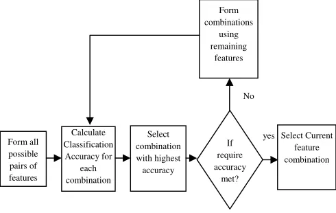
Figure 1: Proposed Feature Selection Method
Initially, all the features are ranked with the use of a feature ranking measure and the most important features alone are retained for next the step. After selecting some top
features from the importance ranking list, the data set is made to classify with only one feature. In this paper, the Support Vector Machine (SVM) classifier is used to test n-feature combinations.
B. Class Separability
Another method used frequently for gene importance ranking is the class separability (CS) [8]. The class separability of gene I can be defined as
0 ) 1)3 2) (4)
1) 67 45)68 45) (5)
2) 9 9 4):
:;<=
67
8 45)6 (6)
For gene i, SBi (the distances between samples of different classes) is the sum of squares of the interclass distances. SWi (the distances of the samples present within the same class) is the sum of squares of the intraclass distances. A larger CS denotes a greater ratio of the interclass distance to the intraclass distance and, therefore, can be used to measure the capability of genes to separate different classes. In fact, the CS used here is similar to the F-statistic that is also widely used for ranking genes in literature (see, e.g., [12], [13]). The difference between the CS and the F-statistic F is:
0 >? @ 8 A 3 67 B6 A (7)
Because the term
>? @ 8 A 3 67 B6A (8)
CS equation is a constant for a specific dataset; the CS can be regarded as a simplification of F-statistic. The two methods will guide to the same ranking results for the same data set.
Step 2: Finding the Minimum Gene Subset
From the importance ranking list, after selecting some top genes the data set is attempted to classify with only one gene. Each selected feature is given as input into our classifier. If no good accuracy is obtained, continued classifying the data set with all the possible 2-feature combinations within the selected feature. If still no good accuracy is obtained, this procedure with 2-features combination is repeated and so on, until a good accuracy is obtained.
A. Support Vector Machine (SVM)
SVM is usually used for classification tasks introduced by Cortes [23]. For binary classification SVM is used to find an optimal separating hyper plane (OSH) which generates a maximum margin between two categories of data. To construct an OSH, SVM maps data into a higher dimensional feature space. SVM carry out this nonlinear mapping with the use of a kernel function. Then, a linear OSH is constructed by SVM between two categories of data in the higher feature space. Data vectors that were nearest to the OSH in the higher feature space are called support Form all
possible pairs of features
Calculate Classification
Accuracy for each combination
Select combination with highest accuracy
If require accuracy
met?
Select Current feature combination Form
combinations using remaining
features
vectors (SVs) and contain all information required for classification. In brief, the theory of SVM is as follows [25]. Consider training set C D 4: E) F)7G with each input n i x ; Rn and an associated output yi∈{ -1, +1}. Each input x is firstly mapped into a higher dimension feature space F, by z= (x) via a nonlinear mapping : Rn F. When data are linearly non-separable in F, a vector w ; F exists there and a scalar b which describe the separating hyper plane as:
E) HI? J)K L M A 8 N) OP (9)
where ξ( ≥0) are called slack variable. The hyper plane that most favorably separates the data in F is one that
QPBPQPRSAT ? HI? H K 0?
RULVSWX XY E) HI? J)K L M A 8 N) N)M Z OP
(10)
where C is said to be regularization parameter that finds the tradeoff among maximum margin and minimum classification error. By constructing a Lagrangian, the optimal hyper plane according to previous equation, may be shown as the solution of
Q[4PQPJS 2 \ 9 \)8AT G
)7
9 9 \)\:E)E:@ 4) 4: G
:7 G
)7
RULVSWX XY G E)
)7 \) Z Z ] \)] 0 OP
(11)
where α1,…..,αL are the nonnegative Lagrangian multipliers. The data points i x that correspond to αi>0 are SVs. The weight vector w is then given by
H )! ^(\)E)J) (12)
For any test vector x Rn , the classification output is then given by
E RP_B H? J K L RP_B 9 \)E)@ 4) 4 K L
)! ^(
(13)
To deploy a SVM classifier, a kernel function and its parameters are chosen primarily. The superiority of one kernel over another is so far, not established by any analytical or empirical studies. In the present study, three kernel functions have been applied as follows to build SVM classifiers:
[a] Linear kernel function, K(x,z) = x,z ;
[b] Polynomial kernel function K( x, z) =( x, z +1) dis the degree of polynomial;
[c] Radial basis function @ 4 J `ab c8def ged, h is
the width of the function.
B. SVM kernel functions
The classification ability of feature combinations in gait applications is obtained with first attempt work of SVM kernel function. The three main kernel functions are used for our study here. Partial kernel function, influence to data near test points. The above mentioned kernel functions are briefly
explained in this chapter. The most used kernel function for SVM is Radial Basis Function (RBF).
[a] Radial Basis Function Kernel: The B-Spline kernel is defined on the interval [−1, 1]. It is given by the recursive formula:
i 4 E 1 'j 4 8 E
HkSlS mno HPXk 1)j p 1)q1r
(14)
In the work by Bart Hamers it is given by:
i 4 E s'7 1 j 4'8 E' (15)
Alternatively, Bn can be computed using the explicit expression (Fomel, 2000):
1 4 Bt 9 uA B K Ai v 8A 6 4 KB K A
T 8 i j
67r
(16)
Where x+ is defined as the truncated power function:
4j c4 P 4 w ZZ YXkSlHPRSx (17)
[b] Linear Kernel: The Linear kernel is the simplest kernel function. It is given by the inner product <x,y> in addition with an optional constant c. Kernel algorithms which uses a linear kernel are often equivalent to their non-kernel counterparts.
i 4 E 4yE K W (18)
[c] Polynomial Kernel: The Polynomial kernel is a non-stationary kernel. Polynomial kernels are apt for problems where all the training data is normalized.
i 4 E z 4yE K W (19)
Modifiable parameters are the slope alpha, the constant term c and the polynomial degree d.
C. Extreme Learning Machine
A new learning algorithm called the Extreme Learning Machine for Single-hidden Layer Feed forward neural Networks (SLFNs) supervised batch learning. The output of an SLFN with ~N hidden nodes (additive or RBF nodes) can be represented by
{| } {|)7 ~)• [) L) } } ; € [); € (20)
where [) and L) are the learning parameters of hidden nodes and βi is the weight connecting the ith hidden node to the output node. G(ai,bi,X) is the output of the ith hidden
node with respect to the input x. For the additive hidden node with the activation function g(x):R→R (e.g., sigmoid or threshold), G(ai,bi,X) is given by
• ‚ƒ „ƒ … † ‚‡? … K „‡ „‡; ˆ (21)
The weight vector which connects the input layer to the ith hidden node is ai and the i
th
hidden node’s bias is bi. ai.x represents the inner product of vectors ai and x in R
RBF hidden node with an activation function
g(x):R→R(e.g., Gaussian), G(ai,bi,X) is given by
• ‚ƒ „ƒ … _ „‡dea 8 ‚‡ed „‡; ˆj (22)
In the above equation ai and bi represents the center and impact factor of ith RBF node. The set of all positive real values are indicated by R+. A special case of the SLFN is the RBF network with RBF nodes in its hidden layer. Each RBF node has its own centroid and impact factor and output of it is given by a radially symmetric function of the distance between the input and the center.
In the learning algorithms it uses a finite number of input-output samples for training. Here, N arbitrary distinct samples are considered (xi,ti)∈R
n
x Rm, where xi is an n x 1 input vector and ti is an m x 1 target vector. If an SLFN with
o| hidden nodes can approximate N samples with zero error, it then implies that there exist βi, ai, and bi such that
{| }: {|)7 ~)• [) L: }: X: V A ‰ ? o (23)
Equation (23) can be written compactly as
Š~ ‹ (24)
Where
Š [ ‰ ? ? [{| L ‰ ? ? L{| } ‰ ? ? }{| =
Œ• [ L }Ž • • [{| L{| }• Ž
• [ L }{ • • [{| L{| }{ •{‘{|
(25)
~ ’~
y Ž ~{|y“
{|‘*
and ‹ ŒX
y Ž X{y•
{‘*
(26)
H represents the hidden layer output matrix of the network; the ith column of H is the ith hidden node’s output vector with respect to inputs x1, x2,…, xN and the jth row of H is the output vector of the hidden layer with respect to input xj.
In real applications, the number of training samples, N, is always greater than the number of hidden nodes o|and, therefore, the training error cannot be brought exactly to zero but can come up to a nonzero training error. The hidden node parameters ai and bi (input weights and biases or centers and impact factors) of SLFNs need not be tuned during training and may simply be assigned with random values according to any continuous sampling distribution. Equation (22) then becomes a linear system and the output weights are estimated as
~” Š • ‹ (27)
In the above equation Š •represents that the Moore-Penrose is generalized inverse [15] of the hidden layer output matrix H. The ELM algorithm which consists of only three steps, can then be summarized as
ELM Algorithm: Given a training set
– D }) X) e}) ; € X); €* P A ‰ oF Activation
function g(x), and hidden node numbero|,
[a] Assign random hidden nodes by randomly generating parameters (ai,bi) according to any continuous sampling
distribution, i=1,….,o|
[b] Calculate the hidden layer output matrix H. [c] Calculate the output weightβ: ~” Š • ‹
The universal approximation capability of ELM has been analyzed by Huang et al. [7] using an incremental method and it shows that single SLFNs with randomly generated additive or RBF nodes with a wide range of activation functions can universally approximate any continuous target functions in any compact subset of the Euclidean space Rn. _ 4
j!—˜™ is the sigmoidal function used as activation function in ELM.
[I] Relevance Vector Machine
The relevance vector machine (RVM) classifier [28], is a probabilistic extension of the linear regression model, which provides sparse solutions. It is analogous to the SVM, since it computes the decision function using only few of the training examples, which are now called relevance vectors. However training is based on different objectives.
The RVM model y(x ; w) is output of a linear model with parameters w = (w1, . . . , wN)T , with application of a sigmoid function for the case of classification:
Eš^/ 4 9 › @ 4 4
{
7
(28)
where (x) = 1/(1+exp(−x)). In the RVM, sparseness is achieved by assuming a suitable prior distribution on the weights, specifically a zero-mean, Gaussian distribution with distinct inverse variance n for each weight ωn:
m ›e\ œ o
{
7
› eZ \ (29)
The variance hyperparameters = ( 1,..., N) are assumed to be Gamma distributed random variables:
m \ œ •[QQ[ \ e[ L
{
7
(30)
The parameters a and b are implicitly fixed and usually they are set to zero (a = b = 0), which provides sparse solutions.
Given a training set D4 X F{7 with X ; DZ AF training in RVM is equivalent to compute the posterior distributionm › \eX. However, since this computation is intractable, a quadratic approximation logm › \eX • › 8
ž y › 8 ž is assumed and computed matrix and
vector as:
Ÿ y1 K ¡ (31)
ž Ÿ ¢£¤¥ (32)
with the N × N matrix described as [ ]ij = K(xi, xj ), A = diag( 1, . . . , N), B = diag( 1, . . . , N), n =
yRVM(xn)[1−yRVM(xn)] and ˆt = +B¡1(t−y). The
parameters are set to the values MP that maximize the logarithm of the following marginal likelihood
¦ \ §Y_m \eX
8AT ¨o§Y_T© K ª«†e¬e K ¤¢¬ ¤-
(33)
with C = B-1 + A-1 T . This, gives the following update formula:
\ A 8 \ Ÿ®®ž (34)
yRVM(x) = y(x; ) can be used to estimate the reliability of the classification decision for input x. Values close to 0.5 are near the decision boundary and consequently are unreliable classifications, while values near 0 and near 1 should correspond to reliable classifications. In this experiment, the reliability measure is used
€¯š^/ eT š^/ 4 8 Ae (35)
which uses values near 0 for unreliable classifications and near 1 for reliable classifications.
IV. EXPERIMENTAL RESULTS
In order to evaluate the performance of the RVM algorithm for multicategory cancer diagnosis Lymphoma and Leukemia Datasets are used in this paper. The detains of the dataset is given below
A. Dataset description
[a] Lymphoma dataset
The lymphoma microarray data has three subtypes of cancer, i.e., CLL, FL, and DLCL. When applying the proposed method to this data set, the clustering result with two best partition eigenvectors is obtained. Seen from cluster results the three classes are correctly divided. Then two sets of l=20 genes are selected according to |Ri,1| and |Ri,2| respectively. (Here set have to be two.) From the two sets of 20 genes each, the two-gene combinations is chosen that can best divide the lymphoma data. Two pairs of genes have been found: 1) Gene 1622X and Gene 2328X, and 2) Gene 1622X and Gene 3343X, which perfectly divide the lymphoma data. Since the results are similar to each other, only the result of one group is shown. Gene ID and gene names of the selecting genes in the lymphoma data set are shown in Table I, where the group and the rank of genes are also shown.
TABLE I: GENE IDS (CLIDS) AND GENE NAMES IN THE TWO MICROARRAY DATA SETS
Data set Gene ID/
CLID Gene Name
Gene Rank
G1 G2
Lymphoma
GENE 1622X
*CD63 antigen (melanoma 1 antigen);
Clone=769861
3 /
GENE 2328X
*FGR tyrosine Kinase; Clone=728609
/ 3
GENE 3343X
*mosaic protein LR11=hybrid; Receptor gp250
precursor; Clone=1352833
/ 4
[b] Leukemia dataset
The leukemia data set contains 5000 genes and 38 samples including 11 Acute Myeloid Leukemia (AML) and 27 acute lymphoblastic leukemia (ALL) samples. The original data set is retrievable from: http://www.broad. mit.edu/cgi-bin/cancer/ datasets.cgi. Maximum 10 clusters are calculated because this data set contains only 38 samples.
B. Experimental process
As introduced in [6], for a microarray data with n genes, each ANOVA classifier produces a hyperplane w, which is a vector of n elements, each corresponding to the expression of a particular gene. The absolute magnitude of each element in w can be considered as a measure of the importance of each corresponding gene. Each ANOVA-RVM classifier is first trained with all of the genes, then the gene corresponding to the bottom 10 percent, wij, are removed. Each classifier is then again trained after the removal of genes. This process is repeated with iterations and a rank of all of the genes based on the statistical significance of each class can be obtained.
SVM is a machine classification technique that directly minimizes the classification error without requiring a statistical data model. This technique is popular since its implementation is very easy and achieves consistently high classification accuracy when applied to many real-world classification situations. The SVM algorithm can be used for both classification and regression (model fitting) problems. In classification, an SVM classifier can separate data that are not easily separable in the original data space by mapping data into a higher dimensional (transformed) space. Kernel functions are used by SVM to find a hyperplane that maximizes the distance (margin) between the two classes, while minimizing training error. The resultant model is sparse, depending only on a few training samples (the “support vectors”). The number of support vectors gets increase linearly with the available training data, requiring much higher computational complexity when classifying very large data sets (e.g., tens or hundreds of thousands of input variables).
The SVM was implemented with the use of Platt’s sequential minimal optimization algorithm in commercial software (Matlab, ver. 5.0; The Math Works, Natick, MA). For classification of the gene expression data, Gaussian (nonlinear) kernels of various widths were tested, and a Gaussian kernel with width = √(2 × number of input variables) was chosen that gave the highest area under the receiver operating characteristic curve using 10-fold cross-validation.
1.0) only through postprocessing. In classification, RVM gives output as probabilities of class membership rather than point estimates like SVM. This gives a conditional distribution that permits the expression of uncertainty in the prediction.
The RVM was implemented with the use of a commercially available algorithm (SparseBayes ver. 1.0; Microsoft Research, Cambridge, UK, for Matlab, The Math Works). For classification of the gene expression data, a Gaussian kernel with width = √(2 × number of input variables) was chosen because it gave the highest ROC curve with 10-fold cross-validation.
[a] Training and Testing Machine Learning Classifiers The proposed technique uses Ten-fold cross-validation to train and test RVM and SVM classifiers to avoid training and testing on the same data. First, affected and healthy genes were randomly divided into 10 approximately equal, exhaustive, and mutually exclusive subsets. Next, classifiers were trained on 9 subsets and then tested on the 10th subset. This sequence was repeated 10 times, using each subset serving as the test set one time, so that each tested gene was never part of its training set and was tested only once. The test results from tested genes were then used to plot the bias-corrected ROC curve. Sensitivities at 75% and 90% specificities are calculated and tabulated in table 2.
As the dimensionality of the experimental data sets (number of parameters) is comparatively large but the size of the data sets (number of observations) is relatively small, sequential forward selection and backward elimination techniques are used to reduce the data dimension to alleviate
the “curse of dimensionality” (reduced classifier
performance caused by the forced inclusion of irrelevant parameters in the solution set). For the simplicity, for RVM these techniques were carried out using RVM and for SVM these techniques were performed using SVM, although RVM can be optimized using SVM and vice versa. For forward selection, with an empty feature set it is started and
sequentially added parameters that improved the
performance of the feature set the most, until peak performance was reached. For backward elimination, with the full-dimensional feature set it is started and sequentially deleted the parameters that improved the performance of the feature set the most, until performance began to decline.
[b] Sensitivity and Specificity
[image:8.612.320.555.309.671.2]The "sensitivity" and "specificity" are medical analysis terms in screening tests for diseases. When a single test is performed on a person, the respective person may in fact have the disease or the person may be disease free. The test result may be positive, representing the presence of disease, or the test result may be negative, indicating the absence of the disease. The Table II below displays test results in the columns and true status of the person being tested in the rows.
TABLE II: MEDICAL ANALYSIS POSSIBILITY GRAPH
Test Result (T)
Positive
(+) Negative (−)
True status of nature (S)
Disease (+) a b
No Disease (−) c d
Though these tests are normally quite accurate, they still make errors that may need to account for.
Sensitivity: It can be defined as the probability that the
test says a person has the disease when in fact they do have the disease. This is P(T- |S+ ) =
+j°. Sensitivity is a measure
of how likely it is for a test to pick up the presence of a disease in a person who has it.
Specificity: It can be defined as the probability that the
test says a person does not have the disease when in fact they are disease free. This is P(T- |S- ) =±j
C. Results for Lymphoma dataset
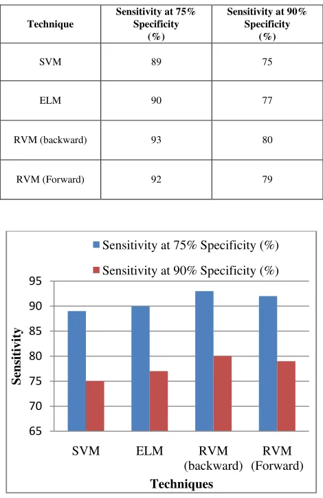
The sensitivity of the different machine learning approaches for the two different specificities are observed and tabulated in table III for the Lymphoma datset. The RVM observations are made for both the forward and backward techniques as explained before. The observed sensitivity is plotted in graph and shown in fig 2.
TABLE III: SENSITIVITIES AT FIXED SPECIFICITIES FOR CLASSIFYING ANCER AFFECTED GENES FROM HEALTHY GENES OF LYMPHOMA DATASET
Technique
Sensitivity at 75% Specificity
(%)
Sensitivity at 90% Specificity
(%)
SVM 89 75
ELM 90 77
RVM (backward) 93 80
RVM (Forward) 92 79
Figure 2: Comparison of sensitivity of finding defected genes among three approaches
SVM ELM RVM
(backward)
RVM (Forward)
S
en
si
ti
v
it
y
Techniques
Sensitivity at 75% Specificity (%)
TABLE IV: TESTING ACCURACY (%) FOR THE SVM, ELM AND RVM ALGORITHMS ON THE LYMPHOMA DATASET
# Genes SVM ELM RVM
(backward)
RVM (Forward)
10 83.21 85.25 86.32 87.94
20 83.92 85.94 86.56 88.57
30 84.55 86.22 87.69 89.31
40 85.17 86.56 88.01 90.18
50 85.94 87.34 88.65 91.34
60 86.57 88.01 88.92 91.95
70 86.99 88.69 89.55 92.65
80 87.66 89.05 89.99 92.97
90 88.32 89.87 90.57 93.41
100 88.87 90.27 92.12 93.82
Average 86.12 87.72 88.83 91.21
The average testing accuracy of the SVM, ELM and RVM are observed in table IV. The testing accuracy is calculated for the lymphoma dataset by varying the number of gene samples for the input. The testing accuracy for the lymphoma datasets are plotted in graph for comparison and it is shown in fig 3.
Figure 3: Comparison of Average testing accuracy among three approaches for Lymphoma dataset
TABLE V: TRAINING TIME (IN SEC) FOR THE SVM, ELM AND RVM ALGORITHMS ON THE LYMPHOMA
# Genes SVM ELM RVM
(backward)
RVM (Forward)
10 442 425 403 390
20 466 448 422 410
30 482 464 446 431
40 512 486 469 452
50 520 499 472 449
60 534 512 493 479
70 549 528 502 489
80 561 542 527 518
90 587 564 549 530
100 603 582 561 549
Average 525.6 505 484.4 469.7
Figure 4: Comparison of Average training time among three approaches for Lymphoma dataset
The average training time taken by the three different techniques for the lymphoma dataset is compared in figure
D. It clearly shows that the proposed RVM approach
is processed in very less time when comparing with the other two approaches.
[a] Results for Leukemia dataset
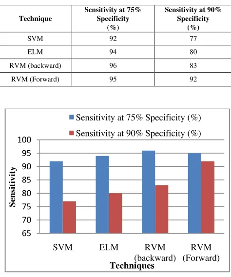
The sensitivity of the different machine learning approaches for the two different specificities for the leukemia dataset are observed and tabulated in table VI. The observed sensitivity is plotted in graph and shown in figure 5.
TABLE VI: SENSITIVITIES AT FIXED SPECIFICITIES FOR CLASSIFYING CANCER AFFECTED GENES FROM HEALTHY GENES OF LEUKEMIA DATASET
Technique
Sensitivity at 75% Specificity
(%)
Sensitivity at 90% Specificity
(%)
SVM 92 77
ELM 94 80
RVM (backward) 96 83
[image:9.612.332.542.50.189.2]RVM (Forward) 95 92
Figure 5: Comparison of sensitivity of finding defected genes among three approaches for Leukemia dataset
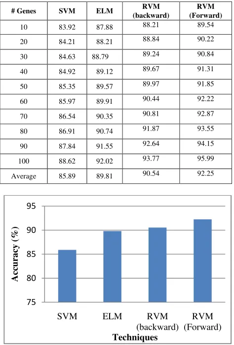
The average testing accuracy of the SVM, ELM and RVM are observed in table VII. The testing accuracy is calculated for the leukemia dataset by varying the number of
SVM ELM RVM
(backward)
RVM (Forward)
A
cc
u
ra
cy
(
%
)
Techniques
400 420 440 460 480 500 520 540
SVM ELM RVM
(backward)
RVM (Forward)
T
ra
in
in
g
T
im
e
(i
n
s
ec
)
Techniques
SVM ELM RVM
(backward)
RVM (Forward)
S
en
si
ti
v
it
y
Techniques
Sensitivity at 75% Specificity (%)
[image:9.612.60.294.341.496.2] [image:9.612.319.556.379.663.2] [image:9.612.59.292.562.690.2]gene samples for the input. The testing accuracy for the leukemia datasets are plotted in graph for comparison and it is shown in figure 6.
TABLE VII: TESTING ACCURACY (%) FOR THE SVM, ELM AND RVM ALGORITHMS ON THE LEUKEMIA DATASET
# Genes SVM ELM RVM
(backward)
RVM (Forward)
10 83.92 87.88 88.21 89.54
20 84.21 88.21 88.84 90.22
30 84.63 88.79 89.24 90.84
40 84.92 89.12 89.67 91.31
50 85.35 89.57 89.97 91.85
60 85.97 89.91 90.44 92.22
70 86.54 90.35 90.81 92.87
80 86.91 90.74 91.87 93.55
90 87.84 91.55 92.64 94.15
100 88.62 92.02 93.77 95.99
Average 85.89 89.81 90.54 92.25
Figure 6: Comparison of Average testing accuracy among three approaches for Lymphoma dataset
TABLE VIII: TRAINING TIME (IN SEC) FOR THE SVM, ELM AND RVM ALGORITHMS ON THE LEUKEMIA DATASET
# Genes SVM ELM RVM
(backward)
RVM (Forward)
10 421 418 394 366
20 457 421 406 384
30 465 450 422 412
40 501 467 440 419
50 524 494 469 447
60 534 503 478 452
70 558 524 492 479
80 564 537 512 498
90 578 541 521 506
100 591 579 554 531
Average 519.3 493.4 468.8 449.4
Figure 7: Comparison of Average training time among three approaches for Lymphoma dataset
The average training time taken by the three different techniques for the leukemia dataset is compared in figure 7. It clearly shows that the proposed RVM approach train the system in very less time when comparing with the other two approaches.
V. CONCLUSION
In this paper, a fast and efficient classification method called the RVM algorithm for a multicategory cancer diagnosis problem based on microarray data is presented. Its performance has been compared for the raw data and ANOVA preprocessed data for the two benchmark medical datasets which are lymphoma and leukemia datasets. It is found that RVM performs better with high accuracy when the data is preprocessed and given as input. The previous methods inevitably involve more classifiers, greater system complexities and computational burden, and a longer training time. RVM can carry out the multicategory classification directly, without any modification. Study results are consistent with our hypothesis that, even when the number of categories for the classification task is large, the RVM algorithm achieves higher classification accuracy than the other algorithms with less training time and a smaller network structure. It can also be seen that RVM achieves more balanced and better classification for individual categories as well. It is also found that the sensitivity of the RVM is high when compared to the SVM and ELM and so this proposed system can be directly implemented for the defective cancer gene classifications.
VI. REFERENCES
[1] M. Ringner, C. Peterson, and J. Khan, “Analyzing
Array Data Using Supervised Methods,”
Pharmacogenomics, vol. 3, no. 3, pp. 403-415, 2002. [2] G.-B. Huang and C.-K. Siew, “Extreme Learning
Machine: RBF Network Case,” Proc. Eighth Int’l Conf. Control, Automation, Robotics, and Vision (ICARCV ’04), Dec. 2004
[3] D. Serre, Matrices: Theory and Applications. Springer-Verlag, 2002.
[4] G.-B. Huang, L. Chen, and C.-K. Siew, “Universal
Approximation Using Incremental Constructive
Feedforward Networks with Random Hidden Nodes,” IEEE Trans. Neural Networks, vol. 17, no. 4, pp. 879-892, 2006.
SVM ELM RVM
(backward)
RVM (Forward)
A
cc
u
ra
cy
(
%
)
Techniques
400 420 440 460 480 500 520 540
SVM ELM RVM
(backward)
RVM (Forward)
T
ra
in
in
g
T
im
e
(i
n
s
ec
)
[image:10.612.57.294.122.471.2] [image:10.612.55.293.535.725.2][5] S. Dudoit, J. Fridlyand, and T.P. Speed, “Comparison of Discrimination Methods for Classification of Tumors Using Gene Expression Data,” J. Am. Statistical Assoc., vol. 97, no. 457, pp. 77-87, 2002.
[6] Runxuan Zhang, Guang-Bin Huang, Narasimhan
Sundararajan, and P. Saratchandran, “ Multicategory Classification Using an Extreme Learning Machine for Microarray Gene Expression Cancer Diagnosis, ” vol 4,no 3,july-september 2007.
[7] M. Schena, D. Shalon, R.W. Davis, and P.O. Brown, “Quantitative Monitoring of Gene Expression Patterns with a Complementary DNA Microarray,” Science, vol. 270, pp. 467-470, 1995.
[8] S. Dudoit, J. Fridlyand, and T.P. Speed, “Comparison of Discrimination Methods for the Classification of Tumors Using Gene Expression Data,” J. Am. Statistical Assoc., vol. 97, pp. 77-87, 2002.
[9] R. Linder, D. Dew, H. Sudhoff, D. Theegarten, K. Remberger, S.J. Poppl, and M. Wagner, “The ’Subsequent Artificial Neural
[10]Network’ (SANN) Approach Might Bring More
Classificatory Power to ANN-Based DNA Microarray Analyses,” Bioinformatics, vol. 20, no. 18, pp. 3544-3552, 2004
[11]G.-B. Huang, Q.-Y. Zhu, and C.-K. Siew, “Extreme Learning Machine: A New Learning Scheme of Feedforward Neural Networks,” Proc. Int’l Joint Conf. Neural Networks (IJCNN ’04), July 2004.
[12]G.-B. Huang and C.-K. Siew, “Extreme Learning Machine: RBF Network Case,” Proc. Eighth Int’l Conf. Control, Automation, Robotics, and Vision (ICARCV ’04), Dec. 2004.
[13]G.-B. Huang and C.-K. Siew, “Extreme Learning Machine with Randomly Assigned RBF Kernels,” Int’l J. Information Technology, vol. 11, no. 1, 2005. [14]G.-B. Huang, Q.-Y. Zhu, K.Z. Mao, C.-K. Siew, P.
Saratchandran, and N. Sundararajan, “Can Threshold Networks Be Trained Directly?” IEEE Trans. Circuits and Systems II, vol. 53, no. 3, pp. 187-191, 2006. [15]M.-B. Li, G.-B. Huang, P. Saratchandran, and N.
Sundararajan, “Fully Complex Extreme Learning Machine,” Neurocomputing, vol. 68, pp. 306-314, 2005.
[16]S. Ramaswamy, P. Tamayo, R. Rifkin, S. Mukherjee, C.-H. Yeang, M. Angelo, C. Ladd, M. Reich, E. Latulippe, J.P. Mesirov, T. Poggio, W. Gerald, M. Loda, E.S. Lander, and T.R. Golub, “Multiclass Cancer Diagnosis Using Tumor Gene Expression Signatures,” Proc. Nat’l Academy Sciences, USA, vol. 98, no. 26, pp. 15149-15154, 2002.
[17] R. Linder, D. Dew, H. Sudhoff, D. Theegarten, K.
Remberger, S.J. Poppl, and M. Wagner, “The ’Subsequent Artificial Neural Network’ (SANN) Approach Might Bring More Classificatory Power to
ANN-Based DNA Microarray Analyses,”
Bioinformatics, vol. 20, no. 18, pp. 3544-3552, 2004. [18]O. Troyanskaya et al., “Missing Value Estimation
Methods for DNA Microarrays,” Bioinformatics, vol. 17, pp. 520-525, 2001.
[19]M. West, C. Blanchette, H. Dressman, E. Huang, S. Ishida, R. Spang, H. Zuzan, J.A. Olson Jr., J.R. Marks, and J.R. Nevins, “Predicting the Clinical Status of Human Breast Cancer by Using Gene Expression Profiles,” Proc. Nat’l Academy of Sciences USA, vol. 98, pp. 11 462-11 467, 2001.
[20]E. Freyhult, P. Prusis, M. Lapinsh, J.E. Wikberg, V. Moulton, and M.G. Gustafsson, “Unbiased Descriptor and Parameter Selection Confirms the Potential of Proteochemometric Modelling,” BMC Bioinformatics, vol. 6, no. 50, 2005.
[21]S. Dudoit, M.J.V.D. Laan, S. Keles, A.M. Molinaro, S.E. Sinisi, and S.L. Teng, “Loss-Based Estimation with Cross-Validation: Application to Microarray Data Analysis and Motif Finding,” Univ of California Berkeley Division of Biostatistics Working Paper
Series, no. 137, 2003,
http://www.bepress.com/ucbbiostat/paper137.
[22]A. Barrier, M.J.V.D. Laan, and S. Dudoit, “Prognosis of Stage II Colon Cancer by Non-Neoplastic Mucosa Gene Expression Profiling,” Univ. of California Berkeley Division of Biostatistics Working Paper Series, no. 179, 2003, http://www.bepress.com/ ucbbiostat/paper179. [23]C. Cortes and V. Vapnik, “Support Vector Networks,”
Mach. Learn., vol. 20, pp. 273–297, 1995.
[24]R. K. Begg, M. Palaniswami and B. Owen, “Support Vector Machines for Automated Gait Classification,” IEEE Trans. Biomed. Eng., vol. 52, no. 5, pp. 828-823, May 2005.
[25]J.M. Khan et al., “Classification and Diagnostic Prediction of Cancers Using Gene Expression Profiling and Artificial Neural Networks,” Nature Medicine, vol. 7, pp. 673-679, 2001.
[26]http://research.nhgri.nih.gov/microarray/Supplement [27]Liyang Wei; Yongyi Yang; Nishikawa, R.M.; Wernick,
M.N.; Edwards, A.; , "Relevance vector machine for automatic detection of clustered microcalcifications", Medical Imaging, IEEE Transactions on Volume: 24 , Issue: 10, Publication Year: 2005 , Page(s): 1278 - 1285 [28]Wen Zhang; Liu, J.; , "Gene Selection for Cancer Classification Using Relevance Vector Machine", Bioinformatics and Biomedical Engineering, 2007. ICBBE 2007, Publication Year: 2007 , Page(s): 184 – 187
[29]Van Staveren HJ, van Veen RL, Speelman OC, Witjes MJ, Star WM, Roodenburg JL. Classification of clinical autofluorescence spectra of oral leukoplakia using an artificial neural network: A pilot study. Oral Oncol 2000;36(3):286–293.
[30]Tumer K, Ramanujam N, Ghosh J, Richards-Kortum R,
Ensembles of radial basis function networks for spectroscopic detection of cervical pre-cancer. IEEE Trans BME 2001;45(8):953–961.
[31]Rovithakis GA, Maniadakis AN, Zervakis M, Fillipidis G, Zakarakis G, Katsamouris AN, Papazoglou TG, Artificial neural networks for discriminating pathologic from normal peripheral vascular tissue. IEEE Trans BME 2001;48(10): 1088–1096.
[32]Agrawal N, Gupta S, et al. Wavelet transform of breast tissue fluorescence spectra—A technique for diagnosis of tumors. IEEE J Selected Topics in Quantum Electronics 2003;9(2): 154–161.
[33]Majumder SK, Ghosh N, Kataria S, Gupta PK.
Nonlinear pattern recognition for laser-induced fluorescence diagnosis of cancer. Lasers Surg Med 2003;33:48–56.
[34]Lin WM, Yuan X, Yuen P, Wei WI, Sham J, Shi PC, Qu J. Classification of in-vivo autofluorescence spectra using support vector machines. J Biomed Opt 2004;9(1):180–186.
AUTHORS
Dr. S. Santhosh Baboo, aged forty two,
has around Nineteen years of postgraduate teaching experience in Computer Science, which includes Six years of administrative experience. He is a member, board of studies, in several autonomous colleges, and designs the curriculum of Under graduate and post graduate programmes. He is a consultant for starting new courses, setting up computer labs, and recruiting lecturers for many colleges. Equipped with a Masters degree in Computer Science and a Doctorate in Computer Science, he is a visiting faculty to IT companies. It is customary to see him at several national/international conferences and training programmes, both as a participant and as a resource person. He has been keenly involved in organizing training programmes for students and faculty members. His good rapport with the IT companies has been instrumental in on/off campus interviews, and has helped the post graduate students to get real time projects. He has also guided many such live projects.Dr. Santhosh Baboo has authored a
commendable number of research papers in
international/national Conference/journals and also guides research scholars in Computer Science. Currently he is Senior Lecturer in the Postgraduate and Research department of Computer Science at Dwaraka Doss Goverdhan Doss Vaishnav College (accredited at ‘A’ grade by NAAC), one of the premier institutions in Chennai.
Mrs. S. Sasikala, done her