R E S E A R C H
Open Access
Stability and bifurcation in a Holling
type II predator–prey model with Allee effect
and time delay
Zaowang Xiao
1, Xiangdong Xie
2*and Yalong Xue
2*Correspondence: [email protected]
2Department of Mathematics
Ningde Normal University, Ningde, China
Full list of author information is available at the end of the article
Abstract
In this paper, we consider a Holling type II predator–prey model incorporating time delay and Allee effect in prey. We discuss the influence of Allee effect on the logistic equation. By analyzing the characteristic equation of the corresponding linearized system, we give the threshold condition for the local asymptotic stability of the system according to the change of birth rate or Allee effect in prey. Using the delay as a bifurcation parameter, the model undergoes a Hopf bifurcation at the coexistence equilibrium when the delay crosses some critical values. In addition, we show that if the Allee effect is large or the birth rate is small, then both predators and prey are extinct. The Allee effect can influence the stability of the system.
MSC: 34C25; 92D25; 34D20; 34D40
Keywords: Predator–prey; Allee effect; Holling type II; Stability; Time delay
1 Introduction
The predator–prey model is one of the basic models between different species in nature which has been widely researched [1–6]. In the natural world, the population generally has a saturation effect. Based on experiments, in order to explain the phenomenon of preda-tion for three different kinds of species, Holling [7] proposed different kinds of functional responses. One of the most important functional responses is Holling type II. For example,
Xu [8] discussed the global dynamics of a delayed predator–prey model with stage
struc-ture and Holling type II functional response for the predator. By constructing a suitable Lyapunov functional, the permanence and global asymptotic stability of the model were derived. Scholars have obtained a large number of interesting results about predator–prey models associated with Holling type II functional response [9–11].
Allee [12] discussed both positive and negative interactions among species, and
pro-posed the concept of the Allee effect. This effect can be caused by difficulties in mate finding [13], inbreeding depression [14], defense to avoid predators, social dysfunction at a low-densities [15]. Moreover, the effect is called to be a weak Allee effect if the density at zero per capita growth is positive, a strong Allee effect if the low-density per capita growth is negative. In the past decades, the Allee effect has always been introduced to explain some
important biological phenomena by many mathematicians and ecologists [16–25]. It was
shown that the low density population can affect the birth rate of the species [26], but the
coefficients of the growth rate are irrelevant to the Allee-type function. Hence, letF(x) be the fertility rate of a speciesx[27]:
F(x) = ax
A+x,
whereadenotes the per capita maximum fertility rate of speciesx;Adenotes the Allee
effect constant of the species. IfA> 0, the fertility rate of the species is zero ifx= 0 and
approaches toaifxis large enough. The value of the parameterAdetermines the growth
rate ofF(x). WhenA= 0, the fertility rateF(x) =ais density independent. Therefore, when considering Allee effect, the logistic equation can be rewritten in the following form:
˙
wheredrepresents the death rate of the species; the intra-specific competition intensity of the species is represented byb;ax/(A+x) is a Michaelis–Menten type function. Obviously, whenA= 0, system (1) is reduced to the traditional logistic equation.
Zu [28] studied a predator–prey system with Allee effect as follows:
˙
and investigated the local asymptotic stability of its equilibria. Meanwhile the author found that the Allee effect of the prey population can bring about unstable or stable
peri-odic fluctuations. Further, Zu and Mimura [29] introduced the Holling type II functional
response into the above system and proposed a system as follows:
˙
The local asymptotic stability of the equilibria was investigated. Also an explicit algorithm was obtained to determine the direction of Hopf bifurcations as well as the stability of the periodic solutions. The phenomenon of periodicity in [29] is similar to that in [28].
In most of ecosystems, maturation, pregnancy, and hunting occur all the time. Hence, time delay due to gestation has been greatly researched as a focus issue in a predator–prey system [2–5,30–32], since the current birth rate of the predator is related to its
consump-tion of prey throughout the past history. Chen and Zhang [33] proposed a predator–prey
of the positive equilibrium. Chen and Chen [36], Wang and Chen [37] considered the bi-furcation phenomenon of a ratio-dependent system incorporating a prey refuge.
However, still seldom scholars consider the dynamic behaviors of a delayed predator– prey system with Allee effect in prey and Holling type II function response. Motivated by the above papers, the main purpose of this paper is to study the stability and Hopf bifurcation of system (3) with delay. More precisely, we study the following model:
˙ x=x
ax
A+x–d–bx
– mxy
1 +hx,
˙
y=nmx(t–τ)y(t–τ) 1 +hx(t–τ) –δy,
(4)
wherexandyrespectively denote the population densities of prey and predators;A,a,b,d,
n,m,h,δare positive constants;τdemonstrates the time delay because of the gestation of the predator;mandhmeasure the effects of capture rate and handling time, respectively;n
is the food conversion rate of the predator;δis the death rate of the predator; (mxy)/(1+hx) is the Holling type II functional response. System (4) is restricted to the following initial conditions:
x(θ) =φ(θ)≥0, y(θ) =ψ(θ)≥0, θ∈[–τ, 0],φ(0) > 0,ψ(0) > 0, (5)
whereφ(θ),ψ(θ) are continuous bounded functions in the interval [–τ, 0].
The rest of this paper is organized as follows: The dynamic behaviors of model (1) and
the existence of equilibria of system (4) are derived in the next section. In Sect.3, we study the local asymptotic stability and Hopf bifurcation of system (4). We end this paper with some examples and a brief discussion.
2 Boundedness and existence of equilibria
In this section, we shall present some preliminary results. Firstly, we study the dynamical behavior of system (1).
Define
a1=Ab+d+ 2 √
Abd.
Theorem 2.1 Let x(t)be a positive solution of system(1)with the initial value x(0) > 0. (1) Ifa<a1,thenlimt→+∞x(t) = 0.
(2) Ifa>a1,then we obtain the following results:
(i) For0 <x(0) <x2,limt→+∞x(t) = 0;
(ii) Forx2<x(0),limt→+∞x(t) =x1,wherex1andx2are defined below.
Proof Note that the equation of model (1) can be rewritten as
˙ x=x
ax
A+x–d–bx
= x
A+x
Denote
f(x) = –bx2+ (a–Ab–d)x–Ad. (7)
Its discriminant is of the form
= (a–Ab–d)2– 4Abd=a2– 2(Ab+d)a+ (Ab–d)2 def=Q1. (8)
Clearly, whenQ1= 0, we have
a0=Ab+d– 2 √
Abd and a1=Ab+d+ 2 √
Abd.
It is easily seen from Eqs. (7), (8) that ifa≤Ab+dandx> 0, thenf(x) < 0; ifAb+d<a<a1
andx> 0, thenf(x) < 0. Further, ifa>a1, thenQ1> 0, hence,f(x) = 0 has two positive roots
x1=
k+√Q1
2b , x2=
k–√Q1
2b , (9)
wherek=a– (Ab+d). If 0 <x<x2, thenf(x) < 0; ifx2<x<x1, thenf(x) > 0; ifx1<x, then
f(x) < 0. The proof is complete.
Remark2.1 IfA= 0, then system (1) reduces to the traditional logistic equationx˙=x(a–
d–bx). For this logistic equation, ifa>d, then every positive solution will tend to a–bd monotonically; ifa≤d, then every positive solution will tend to 0. Note thata≤dimplies thata<a1, then every positive solution of system (1) will tend to 0. Therefore, for system
(1), the species is extinct when the birth rate is less than the death rate. However, we find that when the death rate is smaller than the birth rate, the species is also extinct when
d<a<a1due to the influence of Allee effect. Hence only when the birth rateais larger
thana1, the species maybe not extinct. This shows that the Allee effect may deduce the
instability of system (1).
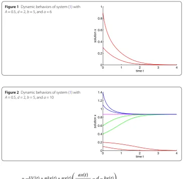
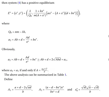
In (1), assume thatA= 0.5,d= 2,b= 5, thena1= 8.9721.
(i) Ifa= 6, that is,a<a1, thenlimt→+∞x(t) = 0(see Fig.1).
(ii) Ifa= 10, that is,a>a1, further if0 <x(0) < 0.2298, thenlimt→+∞x(t) = 0; if
0.2298 <x(0), thenlimt→+∞x(t) = 0.8702(see Fig.2).
In the following, we give the positivity and boundedness of a solution of system (4).
Lemma 2.2 Every solution of system(4)with the initial condition(5)is positive and ulti-mately bounded for all t≥0.
Proof It can be easily proved that every solution of system (4) with (5) remains positive for allt≥0. LetV(t) =nx(t) +y(t–τ), calculating the derivative ofV(t) with respect tot
along the positive solution of system (4), we then have
˙
V(t) =nx˙(t) +y˙(t–τ)
= –δy(t+τ) +nx(t)
ax(t)
A+x(t)–d–bx(t)
Figure 1Dynamic behaviors of system (1) with
A= 0.5,d= 2,b= 5, anda= 6
Figure 2Dynamic behaviors of system (1) with
A= 0.5,d= 2,b= 5, anda= 10
= –δV(t) +nδx(t) +nx(t)
ax(t)
A+x(t)–d–bx(t)
.
By Theorem2.1, there exist some positive constantsBandT such thatV˙(t)≤B–δV(t) for allt≥T. Thuslimt→+∞V(t)≤Bδ; consequently,x(t) andy(t) are ultimately bounded.
The proof is complete.
Letx˙=˙y= 0 in system (4), then
⎧ ⎨ ⎩
x(Aax+x–d–bx) –1+mxyhx= 0,
nmxy
1+hx–δy= 0.
(10)
There always exists a trivial equilibriumE0(0, 0).
Ifa>a1, then system (4) has two boundary equilibriaE1(x1, 0) andE2(x2, 0), where
x1=
k+√Q1
2b and x2=
k–√Q1
2b
withk=a– (Ab+d),Q1=a2– 2(Ab+d)a+ (Ab–d)2.
Further, if
then system (4) has a positive equilibrium
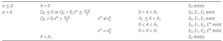
The above analysis can be summarized in Table1.
Define
Ifa≤d, it follows from Table1that there exists only one trivial equilibriumE0of system
(4) for allA. Hence, in the following, we only considera>d. WhenQ0≤0, there does not
Tables1and2show that if the birth rateais relatively small or the Allee effectAis
relatively large, then system (4) only has one trivial equilibriumE0, that is, the predator
and prey will be extinct. If the birth rateais relatively large or the Allee effectAis relatively small, then system (4) has a positive equilibriumE∗, which guarantees the coexistence of system (4).
Table 1 Equilibria of system (4)
0 <a<a1 E0exists
Q0≤0 a>a1 E0,E1,E2exist
Table 2 Equilibria of system (4)
a≤d A> 0 E0exists
a>d Q0≤0 orQ0> 0,x∗≥ab–d 0 <A<A1 E0,E1,E2exist Q0> 0,x∗<a–bd x∗=x0∗ A2≤A<A1 E0,E1,E2exist
0 <A<A2 E0,E1,E2,E∗exist x∗=x0∗ 0 <A<A1 E0,E1,E2,E∗exist
A>A1 E0exists
3 Local stability and Hopf bifurcation 3.1 E0= (0, 0)
Firstly, we discuss the stability ofE0. We obtain the following theorems.
Theorem 3.1 E0of system(4)is locally asymptotically stable.
Proof The variational matrix of system (4) atE0is
V(E0) =
λ+d 0
0 λ+δ
.
Clearly, the characteristic equation of the equilibrium pointE0always has two negative
real roots:λ1= –d,λ2= –δ. The proof is complete.
Therefore,E0is always a locally stable node, which implies that both predators and prey
will become extinct when their population densities lie in the attraction region ofE0. In
particular, if the population density of prey becomes low, then both prey and predators will become extinct.
According to Theorem2.1and the comparison theorem, it is easy to prove the following
theorem.
Theorem 3.2 Assume that a<a1,then E0of system(4)is globally asymptotically stable.
Remark3.1 Whena≤d, it follows from Theorem 3.2that E0 of system (4) is globally
asymptotically stable for any value of the Allee effect. It is easy to show that the condition
a<a1of Theorem3.2is equivalent toa>dandA>A1, which implies that both prey and
predators will go extinct if the Allee effect is strong. Also, we can see that the Allee effect of prey species increases the extinction risk of both predators and prey. Only when the Allee effect is small, the species may not be extinct.
3.2 E1= (x1, 0)
We study the local stability of the boundary equilibriumE1(x1, 0) and have the following
theorem.
Theorem 3.3
(1) Assume thatQ0> 0andA<b(x
∗)2 d hold.
(i) Ifa1<a<a2,thenE1of system(4)is a locally asymptotically stable equilibrium point.
(ii) Ifa>a2,thenE1of system(4)is unstable.
(2) Assume thatQ0> 0andA≥b(x
∗)2
(3) Assume thatQ0≤0holds.Ifa>a1,thenE1of system(4)is locally asymptotically stable.
Proof The variational matrix of system (4) at the equilibrium pointE1is
V(E1) =
and its associated characteristic equation is
First, we consider the following equation:
F1(λ) =λ–
Therefore, we haveλ1< 0, then Eq. (15) has only one negative real root, which implies that
all other roots of Eq. (14) are determined by the following equation:
F2(λ) =λ+δ–
(ii) IfR0< 1, thenN<δ. Suppose that there exists an eigenvalueλwithReλ≥0, then
we have
Reλ=Ne–Re(λ)τcos(Imλ)τ–δ
≤Ne–Re(λ)τ–N< 0. (19)
It is a contradiction, soReλ< 0. This implies that all the real parts of roots of
F2(λ) = 0are negative. HenceE1is a locally asymptotically stable equilibrium.
On the one hand, when Q0> 0, we knowa1=a10=a2 if and only ifA= b(x
Hence, we obtain the following conclusions: (1) Assume thatA<b(xd∗)2, that is,a1<a2<a01, then:
Summarizing the above discussion, we prove Theorem3.3.
3.3 E2= (x2, 0)
Theorem 3.4 Let a>a1,then E2of system(4)is unstable.
Proof The variational matrix of system (4) at the equilibrium pointE2is
V(E2) =
and its associated characteristic equation is
We consider the following equation:
G1(λ) =λ–
2Aax2+ax22
(A+x2)2
+d+ 2bx2= 0. (22)
Then we obtain
λ=2Aax2+ax
2 2
(A+x2)2
–d– 2bx2
= 1
(A+x2)2
–2bx32+ (a–d– 4Ab)x22+ 2A(a–d–Ab)x2–A2d
= – 1
2b2(A+x 2)2
(a–d)Q1+ –a2+Aba+ 2da+Abd–d2
Q1
= –G2(Q1)×
1 2b2(A+x
2)2
, (23)
where
G2(Q1) = (a–d)Q1+ –a2+Aba+ 2da+Abd–d2
Q1. (24)
Let√Q1=t, thent> 0. Hence, Eq. (24) can be rewritten as
g(t) = (a–d)t2+ –a2+Aba+ 2da+Abd–d2t. (25)
Solving the equationg(t) = 0, we can get
t1= 0 and t2=
a2– (Ab+ 2d)a–Abd+d2
a–d =
f1(a)
a–d, (26)
wheref1(a) is defined by (17). Similar to the analysis of Theorem3.3, we obtainf1(a) > 0,
thust2=f1(a)/(a–d) > 0.
Hence, if 0 <t<t2, theng(t) < 0; ift2≤t, theng(t)≥0. That is, if 0 <Q1<t22, then G2(Q1) < 0; ift22≤Q1, thenG2(Q1)≥0. Clearly, the inequalityt22≤Q1does not hold, due
toQ1–t22= –4A 2b2ad
(a–d)2 < 0, which is a contradiction. Thusλ> 0, which implies Eq. (21) has
at least one positive root andE2is unstable. The proof of the theorem is complete.
We summarize the results of Theorems3.3and3.4in Table3. On the other hand, by the
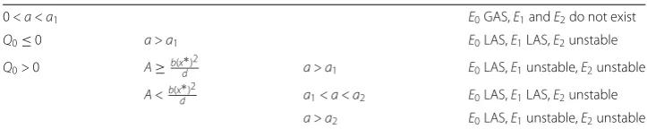
analysis of Sect.2and Theorems3.3and3.4, we also obtain the local asymptotic stability of equilibriaEi,i= 0, 1, 2 (see Table4).
By the definition ofR0and simple computation, from the proofs of Theorems3.3and
3.4, we can obtain the following corollaries.
Corollary 3.1 Let a>d and0 <A<A1,then E1of system(4)is:
(i) unstable if0 <h<nmδ –x11,
(ii) locally asymptotically stable ifh>nmδ –x11.
Table 3 EquilibriaEi,i= 0, 1, 2, of system (4)
Whenτ = 0, by computation, the conditions of Corollaries3.1and3.2are the same as
those of Theorems 1 and 2 [29]. Hence, we extend the local asymptotic stability results
for system (3) to the time delay system (4). It shows that bothE1 andE2 of system (4)
are still locally asymptotically stable under the same condition as those for the nondelay system (3). Therefore, the time delay is harmless for the local stability ofE1andE2. Also,
when considering the birth rateaor the Allee effectAas a parameter, we get the
thresh-old condition for the stability ofE0,i= 0, 1, 2, of system (4). Hence, we obtain some more
precise conditions than those of [29].
3.4 E∗= (x∗,y∗)
Now, to determine the local stability of the interior equilibriumE∗, we use the method
introduced by Beretta and Kuang [38]. Then the characteristic equation atE∗is
p0= –
For the interior equilibriumE∗, we have
Hence, a direct calculation shows that
The above analysis can be summarized in the following theorem.
Theorem 3.6 Let Q0> 0and A<b(x
We present some examples to verify our results.
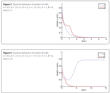
Example4.1 In system (4), assume thatA= 0.5,d= 1,b= 5,m= 5,n= 1,h= 0.1,τ = 1, andδ= 6, thena1= 6.6623.
(i) Ifa= 5, that is,a<a1, it follows from Theorem3.2thatE0is globally asymptotically
stable. Hence, both prey and predators are extinct (see Fig.3).
(ii) Ifa= 8, then system (4) has a boundary equilibriumE1= (0.7702, 0). Note that A= 0.5 < 9.2975 =b(xd∗)2,a1<a< 10.6848 =a2. By Theorem3.3,E1is locally
asymptotically stable (see Fig.4).
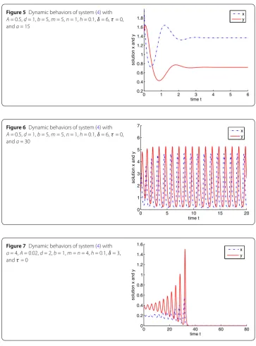
Example4.2 In system (4), assume thatA= 0.5,d= 1,b= 5,m= 5,n= 1,h= 0.1,δ= 6, E∗= (1.3636, 0.7176). By Theorem3.5,E∗is locally asymptotically stable (see Fig.5). (ii) Ifa= 30, thena>a3. Also, we can obtain a positive equilibrium
Figure 3Dynamic behaviors of system (4) with
A= 0.5,d= 1,b= 5,m= 5,n= 1,h= 0.1,τ= 1,δ= 6, anda= 5
Figure 4Dynamic behaviors of system (4) with
A= 0.5,d= 1,b= 5,m= 5,n= 1,h= 0.1,τ= 1,δ= 6, anda= 8
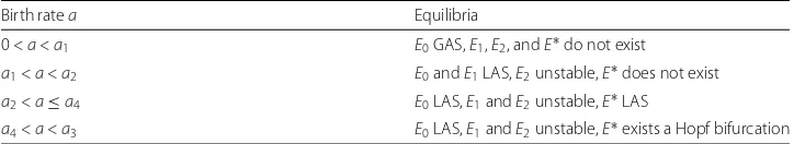
Example4.4 In system (4), assume thatA= 0.5,d= 1,b=m= 5,n= 1,h= 0.1,δ= 6. By calculation, we havea2= 10.6848,a3= 27.2999,a4= 18.4738,Q0= 4.400 > 0,x∗= 1.3636,
andA<b(xd∗)2 = 9.2975.
(i) Ifa= 15andτ = 3. It is easy to show thata2<a<a4and the positive equilibrium is E∗= (1.3636, 0.7176). By Theorem3.6,E∗is locally asymptotically stable (see Fig.8). (ii) Ifa= 15andτ = 15. It is easy to show thata2<a<a4and the positive equilibrium
isE∗= (1.3636, 0.7176). By Theorem3.6,E∗is locally asymptotically stable (see Fig.9).
(iii) Ifa= 20, clearly,a4<a<a3and the positive equilibrium isE∗= (1.3636, 1.5491).
By calculation, we obtainτ0= 0.1387. According to Theorem3.6,E∗is locally
asymptotically stable if0 <τ<τ0and unstable ifτ>τ0, and system (4) undergoes a
Hopf bifurcation atE∗whenτ=τ0, whereτ= 0.07is shown in Fig.10andτ= 0.15
is shown in Fig.11.
5 Conclusion
In this paper, we investigate the stability and Hopf bifurcation of a delayed Holling type II
predator–prey model when the prey is subject to Allee effect. Considering the birth ratea
or the Allee effectAas a parameter, we get the threshold condition for the stability of the equilibria of system (4) and find that the Allee effect or the birth rate plays an important role in the stability of system (4).
Firstly, we analyze the logistic equation (1) with Allee effect, and show that the Allee
Figure 5Dynamic behaviors of system (4) with
A= 0.5,d= 1,b= 5,m= 5,n= 1,h= 0.1,δ= 6,τ= 0, anda= 15
Figure 6Dynamic behaviors of system (4) with
A= 0.5,d= 1,b= 5,m= 5,n= 1,h= 0.1,δ= 6,τ= 0, anda= 30
Figure 7Dynamic behaviors of system (4) with
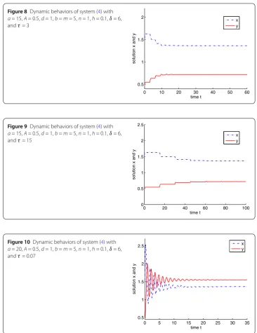
a= 4,A= 0.02,d= 2,b= 1,m=n= 4,h= 0.1,δ= 3, andτ= 0
exists. If the Allee effect is relatively small, with the increase of the birth ratea, the equi-libriumE1changes from the nonexistence to the local asymptotic stability, and eventually
becomes instability. Table4shows that the equilibriumE1changes from instability to local
asymptotic stability, and eventually disappears with the increase of Allee effect.
We also investigate the local asymptotic stability of the coexistence equilibriumE∗and
show that if the time delay passes through some critical values, the equilibriumE∗changes from a stable point to unstable point, and a Hopf bifurcation occurs; further we show periodic solutions.
Letτ= 0, then system (4) is reduced to system (3). If system (3) has only three equilib-rium pointsEi,i= 0, 1, 2.E0(0, 0) is locally asymptotically stable. Further ifE1andE2are
sys-Figure 8Dynamic behaviors of system (4) with
a= 15,A= 0.5,d= 1,b=m= 5,n= 1,h= 0.1,δ= 6, andτ= 3
Figure 9Dynamic behaviors of system (4) with
a= 15,A= 0.5,d= 1,b=m= 5,n= 1,h= 0.1,δ= 6, andτ= 15
Figure 10 Dynamic behaviors of system (4) with
a= 20,A= 0.5,d= 1,b=m= 5,n= 1,h= 0.1,δ= 6, andτ= 0.07
tem (3) has equilibrium pointsEi,i= 0, 1, 2, andE∗. IfE1,E2, andE∗are unstable, then
system (3) admits a limit cycle orE0(0, 0) is globally asymptotically stable. In Table5,
compared with Zu and Mimura [29], we give the threshold condition for the stability of
E0,i= 0, 1, 2, andE∗of system (4) withτ= 0. Therefore, our main results complement and
improve those in [29].
In Theorem3.6, we study the stability and Hopf bifurcation of system (4). The results
of Theorems3.1–3.6are shown in Table6. If the Allee effect is small, the equilibriumE1
changes from the nonexistence to the local asymptotic stability, and eventually becomes
instability with the increase of the birth ratea. On the other hand, the equilibriumE∗
Figure 11 Dynamic behaviors of system (4) with
a= 20,A= 0.5,d= 1,b=m= 5,n= 1,h= 0.1,δ= 6, andτ= 0.15
Figure 12 Dynamic behaviors of the prey in system (4) withA= 0.5,d= 1,b=m= 5,n= 1,
h= 0.1,δ= 6,τ= 0.5, anda= 4 or 8 or 15 or 20
Figure 13 Dynamic behaviors of the predator in system (4) withA= 0.5,d= 1,b=m= 5,n= 1,
h= 0.1,δ= 6,τ= 0.5, anda= 4 or 8 or 15 or 20
and predators are not low, we show the results of Table6in Fig.12and Fig.13with the
same initial values. Change the values of the birth rateafrom zero toa1, the prey species
will stabilize at zero, froma1toa2, the prey species will stabilize atx1. Froma2toa3, the
prey species will stabilize atx∗. Finally, the prey species becomes oscillation ifa4<a<a3.
Table 5 EquilibriaEi,i= 0, 1, 2, andE∗of system (4) withτ= 0
0 <a<a1 E0GAS,E1,E2, andE∗do not exist
Q0≤0 a>a1 E0LAS,E1LAS,E2unstable,E∗does not exist
Q0> 0 A≥b(xd∗)2 a1<a≤a2 E0GAS,E1andE2unstable,E∗does not exist a>a2 E0LAS,E1,E2andE∗unstable
A=b(x∗)2
d a>a1 E0LAS,E1,E2andE∗unstable
A<b(x∗)2
d a1<a<a2 E0LAS,E1LAS,E2unstable,E∗does not exist
a2<a<a3 E0LAS,E1andE2unstable,E∗LAS a>a3 E0LAS,E1,E2, andE∗unstable
Table 6 System (4) withQ0> 0 andA<b(x
∗)2
d
Birth ratea Equilibria
0 <a<a1 E0GAS,E1,E2, andE∗do not exist a1<a<a2 E0andE1LAS,E2unstable,E∗does not exist a2<a≤a4 E0LAS,E1andE2unstable,E∗LAS
a4<a<a3 E0LAS,E1andE2unstable,E∗exists a Hopf bifurcation
Acknowledgements
The authors would like to thank Dr. Xinyu Guan for useful discussion about the mathematical modeling.
Funding
The research was supported by the National Natural Science Foundation of China under Grant (11601085) and the Natural Science Foundation of Fujian Province (2017J01400).
Competing interests
The authors declare that there is no conflict of interests.
Authors’ contributions
All authors contributed equally to the writing of this paper. All authors read and approved the final manuscript.
Author details
1College of Mathematics and Computer Science, Fuzhou University, Fuzhou, China.2Department of Mathematics Ningde
Normal University, Ningde, China.
Publisher’s Note
Springer Nature remains neutral with regard to jurisdictional claims in published maps and institutional affiliations.
Received: 21 June 2018 Accepted: 27 July 2018 References
1. Shi, C.L., Chen, X.Y., Wang, Y.Q.: Feedback control effect on the Lotka–Volterra prey–predator system with discrete delays. Adv. Differ. Equ.2017, Article ID 373 (2017)
2. Chen, F.D., Ma, Z.Z., Zhang, H.Y.: Global asymptotical stability of the positive equilibrium of the Lotka–Volterra prey–predator model incorporating a constant number of prey refuges. Nonlinear Anal., Real World Appl.13(6), 2790–2793 (2012)
3. Ma, Z.Z., Chen, F.D., Wu, C.Q., Chen, W.L.: Dynamic behaviors of a Lotka–Volterra predator–prey model incorporating a prey refuge and predator mutual interference. Appl. Math. Comput.219(15), 7945–7953 (2013)
4. Chen, F.D., Chen, W.L., Wu, Y.M., Ma, Z.Z.: Permanence of a stage-structured predator–prey system. Appl. Math. Comput.219(17), 8856–8862 (2013)
5. Chen, L.J., Chen, F.D.: Dynamic behaviors of the periodic predator–prey system with distributed time delays and impulsive effect. Nonlinear Anal., Real World Appl.12(4), 2467–2473 (2011)
6. Chen, F.D., Xie, X.D., Miao, Z.S., Pu, L.Q.: Extinction in two species nonautonomous nonlinear competitive system. Appl. Math. Comput.274, 119–124 (2016)
7. Holling, C.S.: The functional response of predator to prey density and its role in mimicry and population regulation. Can. Entomol., Suppl.97(S45), 5–60 (1965)
8. Xu, R.: Global stability and Hopf bifurcation of a predator–prey model with stage structure and delayed predator response. Nonlinear Dyn.67(2), 1683–1693 (2012)
10. Lin, Q.X., Xie, X.D., Chen, F.D., Lin, Q.F.: Dynamical analysis of a logistic model with impulsive Holling type-II harvesting. Adv. Differ. Equ.2018, Article ID 112 (2018)
11. Chen, L.J., Chen, F.D., Chen, L.J.: Qualitative analysis of a predator–prey model with Holling type II functional response incorporating a constant prey refuge. Nonlinear Anal., Real World Appl.11(1), 246–252 (2010)
12. Allee, W.C.: Animal Aggregations: A Study in General Sociology. University of Chicago Press, Chicago (1932) 13. Kuussaari, M., Saccheri, I., Camara, M., Hanski, I.: Allee effect and population dynamics in the Glanville fritillary
butterfly. Oikos82, 384–392 (1998)
14. Stephens, P.A., Sutherland, W.J.: Consequences of the Allee effect for behaviour, ecology and conservation. Trends Ecol. Evol.14(10), 401–405 (1999)
15. Courchamp, F., Grenfell, B., Clutton-Brock, T.: Population dynamics of obligate cooperators. Proc. R. Soc. Lond. B 266(1419), 557–563 (1999)
16. Liu, X.S., Dai, B.X.: Dynamics of a predator–prey model with double Allee effects and impulse. Nonlinear Dyn.88(1), 685–701 (2017)
17. Biswas, S., Sasmal, S.K., Samanta, S., Saifuddin, M., Pal, N., Chattopadhyay, J.: Optimal harvesting and complex dynamics in a delayed eco-epidemiological model with weak Allee effects. Nonlinear Dyn.87(3), 1553–1573 (2017) 18. Manna, D., Maiti, A., Samanta, G.P.: A Michaelis-Menten type food chain model with strong Allee effect on the prey.
Appl. Math. Comput.311, 390–409 (2017)
19. Zu, J., Mimura, M., Wakano, J.Y.: The evolution of phenotypic traits in a predator–prey system subject to Allee effect. J. Theor. Biol.262(3), 528–543 (2010)
20. González-Olivares, E., Rojas-Palma, A.: Multiple limit cycles in a Gause type predator–prey model with Holling type III functional response and Allee effect on prey. Bull. Math. Biol.73(6), 1378–1397 (2011)
21. Guan, X.Y., Liu, Y., Xie, X.D.: Stability analysis of a Lotka–Volterra type predator–prey system with Allee effect on the predator species. Commun. Math. Biol. Neurosci.2018, Article ID 9 (2018)
22. Wu, R.X., Li, L., Lin, Q.F.: A Holling type commensal symbiosis model involving Allee effect. Commun. Math. Biol. Neurosci.2018, Article ID 6 (2018)
23. Lin, Q.F.: Allee effect increasing the final density of the species subject to the Allee effect in a Lotka–Volterra commensal symbiosis model. Adv. Differ. Equ.2018, Article ID 196 (2018).
24. Lin, Q.F.: Stability analysis of a single species logistic model with Allee effect and feedback control. Adv. Differ. Equ. 2018, Article ID 190 (2018)
25. Chen, B.G.: Dynamic behaviors of a commensal symbiosis model involving Allee effect and one party can not survive independently. Adv. Differ. Equ.2018, Article ID 212 (2018)
26. Pal, P.J., Saha, T., Sen, M., Banerjee, M.: A delayed predator–prey model with strong Allee effect in prey population growth. Nonlinear Dyn.68(1–2), 23–42 (2012)
27. Ferdy, J.B., Molofsky, J.: Allee effect, spatial structure and species coexistence. J. Theor. Biol.217(4), 413–424 (2002) 28. Zu, J.: Global qualitative analysis of a predator–prey system with Allee effect on the prey species. Math. Comput.
Simul.94, 33–54 (2013)
29. Zu, J., Mimura, M.: The impact of Allee effect on a predator–prey system with Holling type II functional response. Appl. Math. Comput.217(7), 3542–3556 (2010)
30. Li, Z., He, M.X.: Hopf bifurcation in a delayed food-limited model with feedback control. Nonlinear Dyn.76(2), 1215–1224 (2014)
31. Li, Z., Han, M.A., Chen, F.D.: Global stability of a predator–prey system with stage structure and mutual interference. Discrete Contin. Dyn. Syst., Ser. B19(1), 173–187 (2014)
32. Yang, K., Miao, Z.S., Chen, F.D., Xie, X.D.: Influence of single feedback control variable on an autonomous Holling-II type cooperative system. J. Math. Anal. Appl.435(1), 874–888 (2016)
33. Chen, Y.M., Zhang, F.Q.: Dynamics of a delayed predator–prey model with predator migration. Appl. Math. Model. 37(3), 1400–1412 (2013)
34. Yuan, S.L., Ji, X.H., Zhu, H.P.: Asymptotic behavior of a delayed stochastic logistic model with impulsive perturbations. Math. Biosci. Eng.14(5–6), 1477–1498 (2017)
35. Song, Y.L., Yin, T., Shu, H.Y.: Dynamics of a ratio-dependent stage-structured predator–prey model with delay. Math. Methods Appl. Sci.40(18), 6451–6467 (2017)
36. Chen, L.J., Chen, F.D.: Global stability and bifurcation of a ratio-dependent predator–prey model with prey refuge. Acta Math. Sinica (Chin. Ser.)57(2), 301–310 (2014)
37. Wang, Y.Q., Chen, L.J., Gao, H.Y.: Global analysis of a ratio-dependent predator–prey system incorporating a prey refuge. J. Nonlinear Funct. Anal.2017, 1–26 (2017)
38. Beretta, E., Kuang, Y.: Geometric stability switch criteria in delay differential systems with delay dependent parameters. SIAM J. Math. Anal.33(5), 1144–1165 (2002)