NUMERICAL SOLUTION OF BERGERS’ EQUATION IN A ONE-DIMENSIONAL GROUNDWATER RECHARGE BY SPREADING USING FINITE DIFFERENCE METHOD

(1)

NUMERICAL SOLUTION OF BERGERS’ EQUATION

IN A ONE-DIMENSIONAL GROUNDWATER

RECHARGE BY SPREADING USING FINITE

DIFFERENCE METHOD

Ravi N. Borana

1

, V. H. Pradhan

2

, and M. N. Mehta

3

1

Department of Mathematics,

Bhavan’s Sheth R. A. College of Science, Ahmedabad, (India)

2, 3

Department of Applied Mathematics and Humanities,

S. V. National Institute of Technology, Surat, (India)

ABSTRACT

The ground water is recharged by spreading of the water in downward direction and the moisture content of soil increases. The mathematical formulation of the phenomena leads to the governing equation, which is a non-linear partial differential equation in the form of Burgers’ equation which has been solved by using Crank-Nicolson finite difference scheme with appropriate initial and boundary conditions. The average diffusivity coefficient over the whole range of moisture content is regarded as constant. It is concluded that the moisture content of soil increases with the depth

Z

and increasing time

T

. The numerical solutions of the governing equation have been obtained in the form of tables and graphs by using MATLAB coding. The numerical solution represents moisture content distribution in the vertically downward direction at any depth

Z

for time

0 T



.

This type of problems appears particularly in soil mechanics, hydrology, ceramic engineering and petroleum technology.

Keywords: Moisture Content, Unsaturated Porous Medium, Burgers’ Equation, Finite Difference

Method.

I. INTRODUCTION

The soil plays one of the most important roles in the hydrological cycle. Moisture content is the quantity of

water contained in a material, such as soil (called soil moisture). The saturated zone is one in which the entire

void space is occupied by water. In the unsaturated zone only part of the void space is occupied by water. The

phreatic surface (or water table), is an imaginary surface that bounds the saturated zone from above. It separates

the saturated and unsaturated zones. In the dry soil there is no moisture, so the value of moisture content is 0 in

the unsaturated porous medium and its value is 1, when the porous medium is fully saturated by water. The

range of moisture content is [0, 1].The region of the unsaturated soil is known as Vadose zone (or unsaturated

(2)

the water table the void space is practically fully saturated for a certain distance. This region is called the

capillary fringe, or capillary zone. The term moisture content is used in hydrogeology, soil sciences and soil

Mechanics. In saturated ground water aquifers, all available pore spaces are filled with water. Above a capillary

fringe pore spaces have air in them too. If the porous medium is soil, water content is same as the soil moisture.

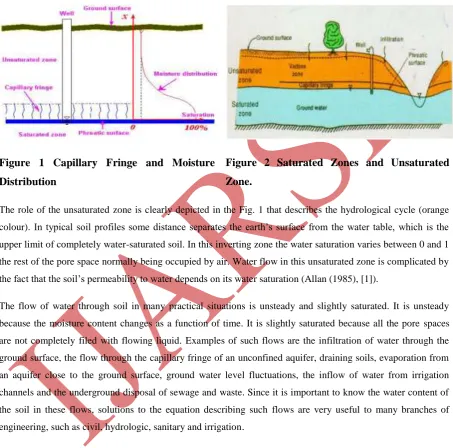
Figure 1 Capillary Fringe and Moisture

Distribution

Figure 2 Saturated Zones and Unsaturated

Zone.

The role of the unsaturated zone is clearly depicted in the Fig. 1 that describes the hydrological cycle (orange

colour). In typical soil profiles some distance separates the earth’s surface from the water table, which is the

upper limit of completely water-saturated soil. In this inverting zone the water saturation varies between 0 and 1

the rest of the pore space normally being occupied by air. Water flow in this unsaturated zone is complicated by

the fact that the soil’s permeability to water depends on its water saturation (Allan (1985), [1]).

The flow of water through soil in many practical situations is unsteady and slightly saturated. It is unsteady

because the moisture content changes as a function of time. It is slightly saturated because all the pore spaces

are not completely filed with flowing liquid. Examples of such flows are the infiltration of water through the

ground surface, the flow through the capillary fringe of an unconfined aquifer, draining soils, evaporation from

an aquifer close to the ground surface, ground water level fluctuations, the inflow of water from irrigation

channels and the underground disposal of sewage and waste. Since it is important to know the water content of

the soil in these flows, solutions to the equation describing such flows are very useful to many branches of

engineering, such as civil, hydrologic, sanitary and irrigation.

The phenomenon of the one dimensional vertical groundwater recharge by spreading is of great importance to

hydrologists, agriculturists and for the people related with water resources sciences. The hydrological situation

of such problem is confirmed by Verma (1973). The water infiltration system, seepage problem and the

underground disposal of wastewater, all harmonize with the flow discussed in the present paper.

This phenomenon has been discussed by many researchers from the different viewpoints. Here are some of the

examples-Klute (1952)[2], has reduced diffusion equation to an ordinary differential equation and

(3)

a linear diffusion coefficient. Swartzendruber uses Philip’s (1970) method to get graphical illustration of the

mathematical solution for horizontal water function. Verma (1969)[3], has employed Laplace transformation

technique to solve this problem; Mehta (1975)[4], has obtained an approximate solution considering average

diffusivity coefficient of the whole range of moisture content and treated as small constant by the method of

singular perturbation technique. Allan (1985) had reviewed modification, assumptions and different techniques

used by other researchers. Hari Prasad et al. (2001)[5], had developed a numerical model to simulate water flow

through unsaturated zones and study the effect of unsaturated soil parameters on water movement during

different processes such as gravity drainage and infiltration. They had developed a numerical model to simulate

moisture flow through unsaturated zones using the finite element method. This model is also applied to predict

moisture contents during a field internal drainage test. De varies and Simmers (2002) had discussed processes

and challenges principally on recharge of unconfined aquifers, then the most readily available and affordable

source of water in (semi-unconfined aquifers), (semi-) arid regions. Faybishenko (2004) has given review of the

theoretical concepts, presented results, and provided perspectives on investigations of flow and transport in

unsaturated heterogeneous soils and fractured rock, using the methods of nonlinear dynamics and determine

chaos. Patel and Mehta (2006) [6], have studied ground water recharge by spreading in vertical downward

direction. They constitute governing differential equation as Burgers equation, with permeability as nonlinear

function of moisture content. Mishra and Verma (1973) obtained a similarity solution of a unidimensional

vertical ground water recharges through porous media. Mehta and Saroj (2007) [7], have considered aqueous

conductivity directly proportional to depth, moisture content and inversely proportional to time. They obtained

an approximate solution for the vertical groundwater recharge problem in slightly saturated porous media by

using small parameter method.

The moisture in wet porous media migrates generally due to the following causes: the total pressure gradient,

the moisture content gradient, and the temperature gradient. Under negligible total pressure gradient or in a

medium with poor permeability, the moisture migrations caused by the later two causes are prevailing. Hunt

1978; Piatnitskii 2005; Mikelic 2009; Meher 2010 ([8] and [9]) discussed it from different point of view. In the

present paper the mathematical formulation of the moisture content phenomena yields a non-linear partial

differential equation in the form of Burgers’ equation, its numerical solution has been obtained by using Finite

Difference methods. The diffusivity coefficient is assumed to be constant over a whole range of moisture

content and permeability of the porous media is assumed to be varying directly to the square of the moisture

content (Verma (1972), [10]).

II. STATEMENT OF THE PROBLEM

In the investigated model it is considered that the ground water recharge takes place over a large basin (taken as

a homogeneous porous medium) of such geological configuration that the sides are limited by rigid boundaries

while the bottom is confined by a thick layer of water table. Under these circumstances, water, from the

spreading grounds, will flow vertically downwards through the unsaturated porous medium (negligible amount

of water may spread in other directions; hence, it is ignored comparing to the large size of basin). That is initial

(4)

coefficient is equivalent to its average value over the whole range of moisture content; it is small enough

constant and, regarded as a perturbation parameter. Further the permeability of the medium is considered to vary

directly as square of the moisture content. For the present analysis the following assumptions have been made

(Hari Prasad et al. (2001)): The medium is homogenous. There is no air resistance to the flow (i.e. the porous

medium contains only the flowing liquid water and empty voids). The air in the void space is approximately at

atmospheric pressure i.e. air is stationary. The soil properties are taken to be constant. The flowing liquid

(water) is considered continuous at a microscopic level, incompressible and isothermal. The initial moisture

content is uniform throughout the soil profile and the moisture content at the soil surface is constant and near

saturation also rainfall or irrigation rate is constant. Darcy’s law is applicable.

III. MATHEMATICAL FORMULATION

The motion of water in isotropic, homogenous porous medium is given by Darcy’s law (Bear 1972) as,

V

  

K



(1)

Where,

V

is the volume flux of the moisture content,

K

is the coefficient of aqueous conductivity and





is the gradient of the whole (total) moisture potential.

The motion of water flow through unsaturated porous media is governed by the continuity equation,



s



M

t

 



 



(2)

Where,



_s

is the bulk density of medium on dry weight basis,



is the moisture content at any depth

z

on

a dry weight basis and

M

is the mass of flux of moisture at any time

t



0 .

Here, moisture content





PS

(John 1976),where,

P

is the porosity of the medium and

S

is the saturation of the water.

Using incompressibility of the water, from the equations (1) and (2) it follows that



s



_{ }

_

_

V

K

t

 







 

 





(3)

where,



is the flux density of the medium. Since, in the present problem, flow takes place only in the vertical

direction, therefore equation (3) reduces to:





s

K

Kg

t

z















_







_

















(4)

Where, ‘



’

is the pressure (capillary) potential,

g

is the gravitation constant, and

 

 

zg

the positive

(5)

Considering



and



to be connected by a single valued function, equation (4) [11], may be written as

s

K

D

g

t

z







_









_









_



_



(5)

where,

s s

D



K



 

K













and is called the diffusivity coefficient. Replacing

D

by its average value

‘

D

_a

’

over the whole range of the moisture content (Mehta 1977) and

K





2 (Mehta 2006)

i.e.

K



K

₀



2

,

where ‘

K

₀

’ is constant. Hence, equation (5) becomes

2

0 2

2

_a

s

gK

D

t

z





_







_



_



(6)

Substituting

2

₀ ₁

s

gK

K





, equation (6) becomes

2

1 a 2

K

D

t

z



_





_



_



(7)

For the sake of simplicity of the problem, the value of the constant

K

₁



1 is considered.

IV. CRANK-NICOLSON SCHEME FOR THE GOVERNING EQUATION

To obtain the numerical solution of the equation (7), choose new variables

Z

z

L



&

1 t

T



and

0  

z

L

, hence,

0  

Z

1. And also

0  

T

1

Hence, the equation (7) can be written as

2

; 0

1

a

D

Z

T

Z



_





_



_



_{ }



(8)

The expression (8) is the governing non-linear partial differential equation known as Burgers’ equation for the

moisture content distribution phenomenon. The term

D

_a

is an average diffusivity coefficient over the whole

range of the moisture content. Consider



₀ as the initial moisture content. Since, the moisture content of the

soil increases as the depth Z increases (Ramakant (2010) [8]); considered the initial moisture content as

(6)





0

 

1

, 0

Z

; 0

1 Z

Z

Ze

Z











 

(9)

Also the moisture content at the top (i.e. depth Z = 0), in the unsaturated porous media is very small and at the

bottom the moisture content of soil will be fully saturated. So, it is suitable to choose the boundary conditions as





 

0

0,

0.01 1,

1

0

1 T

T





 

(10)

The Crank-Nicolson finite difference scheme to the governing equation (8) with the appropriate conditions of

the expression (9) and expression (10) has been employed as under ([13], [14]).

Introducing, the stability ratio

 

2

T

r

Z







, we have, for

i



1

,

 





1 1, 1 1 2, 1 1 1,

1, 1, 1,

2 2 2

1 2, 1

1, 1,

2 2

1 1, 1, 2, 1, 1, ₂

2

1

2

1

3

2

1 0.02 2

... 11

2 with

0.02

2

4

n n n

n

n n

n n n n

n

a a a

a a

D

Z

D

Z

D

Z

r

D

Z

D

Z

r

Z

D



       















_

 



_



_





_



_

 



_

















_

_



_





_



_





_















_









 

_a





_2,_n



3 

_1,_n



0.02 



_

For

2   

i

R

1 ,

 

1 1, 1 , 1 1 1, 1

, ,

2 2

1 1, , 1 1,

, ,

2 2

1 , , 1,

, ₂

1

2

1

2 ... 12

2

2 with

.

4

i n a i n i n

i n i n

i n a i n i n

i n i n

i n i n i n

i n

a a

D

Z

D

Z

r

D

Z

D

Z

r



            



_

_



_



_



_



_

_



_







































_





_



_



_



_





_

















_









_i__1,_n



 

Z

2 D

_a





_i__1,_n



2 

_{i n}_,





_i__1,_n





_

For

i



R

,

 





1 1, 1 1 , 1 1 1,

, , ,

2 2 2

1 , 1

, ,

2 2

1 , , , 1,

, ₂

1

2

1

3

2

1

3

4 ... 13

2

2 with

.

2

4

R n R n R n

R n R n R n

R n

R n R n

R n R n R n R n

R n

a a a

a a

a

D

Z

D

Z

D

Z

r

D

Z

D

Z

r

Z

D



          



_

_



_



_{ }

_



_{ }



_

_





































_

 



_



_





_













_





  



_R__1,_n



3 

_{R n}_,



2 



_

The expressions (11), (12) and (13) represent the Crank-Nicolson finite difference scheme about the point



, 1



2

,

i i n

(7)

the whole range of the moisture content has been considered as a constant value 1. The solution of the

expression (8) in form of tables and graphs is obtained using MATLAB coding.

V. NUMERICAL AND GRAPHICAL REPRESENTATION OF THE SOLUTION

0 0.1 0.2 0.3 0.4 0.5 0.6 0.7 0.8 0.9 1 0

0.1 0.2 0.3 0.4 0.5 0.6 0.7 0.8 0.9 1

dZ=0.025 , dT=0.0003 r = 0.48

The values of Z

M

o

is

tu

re

C

o

n

te

n

t

T

h

e

ta

(Z

,

T

)

T= 0.06 T= 0.12 T= 0.18 T= 0.24 T= 0.30

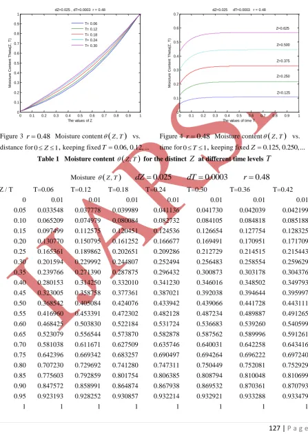
Figure 3

r



0.48

Moisture content



Z T,



vs. distance for 0 Z 1

, keeping fixed

T0.06, 0.12,...

0 0.1 0.2 0.3 0.4 0.5 0.6 0.7 0.8 0.9 1 0

0.1 0.2 0.3 0.4 0.5 0.6 0.7

The values of time T

M

o

is

tu

re

C

o

n

te

n

t

T

h

e

ta

(Z

,

T

)

dZ=0.025 dT=0.0003 r = 0.48

Z=0.625

Z=0.500

Z=0.375

Z=0.250

Z=0.125

Figure 4

r



0.48

Moisture content



Z T,



vs. time for 0 T 1

, keeping fixed

Z0.125, 0.250,...

Table 1 Moisture content 



Z T,



for the distinct

Z

at different time levels

T

Moisture 



Z T,



dZ



0.025 dT



0.0003

r



0.48

Z / T T=0.06 T=0.12 T=0.18 T=0.24 T=0.30 T=0.36 T=0.42

0 0.01 0.01 0.01 0.01 0.01 0.01 0.01

0.05 0.033548 0.037778 0.039989 0.041136 0.041730 0.042039 0.042199

0.10 0.065209 0.074979 0.080084 0.082732 0.084105 0.084818 0.085188

0.15 0.097499 0.112575 0.120451 0.124536 0.126654 0.127754 0.128325

0.20 0.130770 0.150795 0.161252 0.166677 0.169491 0.170951 0.171709

0.25 0.165361 0.189862 0.202651 0.209286 0.212729 0.214515 0.215443

0.30 0.201594 0.229992 0.244807 0.252494 0.256483 0.258554 0.259629

0.35 0.239766 0.271390 0.287875 0.296432 0.300873 0.303178 0.304376

0.40 0.280153 0.314250 0.332010 0.341230 0.346016 0.348502 0.349793

0.45 0.323005 0.358758 0.377361 0.387021 0.392038 0.394644 0.395997

0.50 0.368542 0.405084 0.424076 0.433942 0.439066 0.441728 0.443111

0.55 0.416960 0.453391 0.472302 0.482128 0.487234 0.489887 0.491265

0.60 0.468425 0.503830 0.522184 0.531724 0.536683 0.539260 0.540599

0.65 0.523079 0.556544 0.573870 0.582878 0.587562 0.589996 0.591261

0.70 0.581038 0.611671 0.627509 0.635746 0.640031 0.642258 0.643416

0.75 0.642396 0.669342 0.683257 0.690497 0.694264 0.696222 0.697240

0.80 0.707230 0.729692 0.741280 0.747311 0.750449 0.752081 0.752929

0.85 0.775603 0.792859 0.801754 0.806385 0.808794 0.810048 0.810699

0.90 0.847572 0.858991 0.864874 0.867938 0.869532 0.870361 0.870793

0.95 0.923193 0.928252 0.930857 0.932214 0.932921 0.933288 0.933479

(8)

0 0.1 0.2 0.3 0.4 0.5 0.6 0.7 0.8 0.9 1 0

0.1 0.2 0.3 0.4 0.5 0.6 0.7 0.8 0.9 1

dZ=0.025 dT=0.0005 r = .8

The values of Z

M

o

is

tu

re

C

o

n

te

n

t

T

h

e

ta

(Z

,

T

)

T=0.05 T=0.10 T=0.20 T=0.30 T=0.40

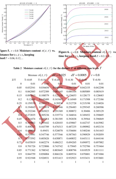
Figure 5.

r



0.8 Moisture content





Z T,



vs.

distance for

0 Z 1

, keeping

fixed

T 0.06, 0.12,...

0 0.1 0.2 0.3 0.4 0.5 0.6 0.7 0.8 0.9 1 0.05

0.1 0.15 0.2 0.25 0.3 0.35 0.4 0.45 0.5 0.55

dZ=0.025 dT=0.0005 r = 0.8

The values of time T

M

o

is

tu

re

c

o

n

te

n

t

T

h

e

ta

(Z

,

T

)

Z=0.6

Z=0.4

Z=0.3 Z=0.5

Z=0.2

Figure 6.

r



0.8 Moisture content





Z T,



vs.

time for

0 T 1

, keeping fixed

Z0.2, 0.3,...

Table 2 Moisture content 



Z T,



for the distinct

Z

at different time levels

T

Moisture 



Z T,



dZ



0.025 dT



0.0005

r



0.8

Z/T T=0.05 T=0.10 T=0.20 T=0.30 T=0.40 T=0.50

0 0.01 0.01 0.01 0.01 0.01 0.01

0.05 0.032541 0.036656 0.040456 0.041729 0.042155 0.042298

0.1 0.062885 0.072389 0.081165 0.084104 0.085089 0.085419

0.15 0.093913 0.108579 0.122118 0.126653 0.128173 0.128683

0.2 0.12601 0.145489 0.163467 0.16949 0.171508 0.172186

0.25 0.159539 0.183373 0.20536 0.212728 0.215198 0.216026

0.3 0.194845 0.222474 0.247946 0.256483 0.259345 0.260306

0.35 0.232246 0.263023 0.291369 0.300872 0.30406 0.305129

0.4 0.272035 0.305236 0.335774 0.346016 0.349452 0.350605

0.45 0.314476 0.349314 0.381305 0.392038 0.39564 0.396849

0.5 0.359802 0.395442 0.428103 0.439067 0.442747 0.443982

0.55 0.408217 0.443789 0.476313 0.487235 0.490902 0.492134

0.6 0.459895 0.49451 0.526078 0.536684 0.540246 0.541443

0.65 0.514981 0.547746 0.577546 0.587563 0.590929 0.592059

0.7 0.573592 0.603626 0.630871 0.640032 0.643111 0.644146

0.75 0.635819 0.662274 0.686212 0.694265 0.696972 0.697882

0.8 0.701726 0.723806 0.743742 0.75045 0.752706 0.753464

0.85 0.771362 0.788342 0.803645 0.808796 0.810529 0.811111

0.9 0.844759 0.856004 0.866126 0.869534 0.870681 0.871066

0.95 0.921948 0.926931 0.931413 0.932923 0.933431 0.933601

(9)

0 0.1 0.2 0.3 0.4 0.5 0.6 0.7 0.8 0.9 1 0

0.1 0.2 0.3 0.4 0.5 0.6 0.7 0.8 0.9 1

dZ=0.025 dT=0.001 r = 1.6

The values of Z

M

o

is

tu

re

C

o

n

te

n

t

T

h

e

ta

(Z

,

T

)

T=0.05 T=0.10 T=0.15 T=0.20 T=0.25

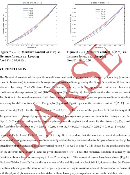
Figure 7

r



1.6 Moisture content





Z T,



vs.

distance for

0 Z 1

, keeping

fixed

T0.05, 0.10,...

0 0.1 0.2 0.3 0.4 0.5 0.6 0.7 0.8 0.9 1 0

0.1 0.2 0.3 0.4 0.5 0.6 0.7 0.8 0.9 1

dZ=0.025 dT=0.0025 r = 4

The values of Z

M

o

is

tu

re

C

o

n

te

n

t

T

h

e

ta

(Z

,

T

)

T=0.10 T=0.20 T=0.30 T=0.40 T=0.50

Figure 8

r



4 Moisture content





Z T,



vs.

distance for

0 Z 1

, keeping

fixed

T0.10, 0.20,...

VI. CONCLUSION

The Numerical solution of the specific one-dimensional vertical groundwater recharge by spreading (moisture

content phenomena) in unsaturated homogeneous porous medium, given by the Burger’s equation (8) has been

obtained by using Crank-Nicolson Finite Difference scheme, with the appropriate initial and boundary

conditions of the expressions (9) and (10). The graphs (Fig. 3 to Fig. 8) clearly indicate that the moisture content

distribution in the one-dimensional fluid flow through unsaturated homogeneous porous medium is steadily

increasing for different timeT0

. The graphs (Fig.4 and Fig.6) represent the moisture content





Z T,



vs. time Tfor 0 T 1, for the fixed distance Z 0.2, 0.3,...

.The nature of the graphs reflect that the height of

the groundwater recharge by spreading in unsaturated homogeneous porous medium is increasing as per the

Figs. 3, 5, 7 and 8 according to the physical phenomenon throughout the domain for the distance 0 Z 1 and the fixed time levels taken as T0.05,T0.10 ,T0.15,T0.20,T0.25,T0.30,T0.40 & T0.50.

From the Table 1 and Table 2, and Fig. 3 to Fig. 8, it is evident that the moisture content distribution in

unsaturated homogeneous porous medium steadily and uniformly increases due to the groundwater recharge by

spreading with the increasing distance (vertical heightZ ) as well as timeT

. It is shown by the graphs and tables

for the different time levels T

and the given distance 0

 Z 1

.

Thus, the numerical solution obtained by the Crank-Nicolson scheme is converging to 1 as Z tending to 1. The numerical results have been shown (Fig.3 to

Fig.8 and Tables 1 and 2) for the distinct values of the stability ratior0.48, 0.8, 1.6, 4 reveals that the Crank-Nicolson scheme gives the solution of Bergers’ equation arising in moisture content phenomenon is consistent

(10)

ACKNOWLEDGEMENT

I am full of gratitude and gratefulness towards my mother institute Bhartiya Vidhya Bhavan, Ahmedabad

Kendra, for giving me an opportunity to begin research work. This work would have been completely

impossible without the constant motivation, support and encouragement of my former Principal C. B. Gemawat.

REFERENCES

[1] M. B. Allen, Numerical modelling of multiphase flow in porous media. Adv. Water Resources, Volume 8, December,

1985, 162-187.

[2] A. A. Klute, A numerical method for solving the flow equation for water in unsaturated materials. Soil Science, 1952,

73-105.

[3] A. P. Verma, The Laplace transform solution of one dimensional groundwater recharge by spreading. Annalidi Geofisica

XXII-1, 1969, 25-31.

[4] M. N. Mehta, A singular perturbation solution of one-dimensional flow in unsaturated porous media with small diffusivity

coefficient, Proc. 1975, FMFP E1 to E4.

[5] K. S. Hari Prasad, M. S. Mohan and M. Shekhar, Modelling Flow Through Unsaturated Zone: Sensitivity to Unsaturated

Soil Properties. Sadhana, Indian Academy of Sciences, 26(6), 2001, 517-528.

[6] M. N. Mehta and Patel T, A solution of Burgers’ equation type one-dimensional Groundwater Recharge by spreading in

Porous Media. The Journal of the Indian Academy of Mathematics, 28(1), 2006, 25-32.

[7] M. N. Mehta and S. R. Yadav, Solution of Problem arising during vertical groundwater recharge by spreading in slightly

saturated Porous Media, Journal of Ultra Scientists of Physical Sciences. Vol.19(3), 2007, 541-546.

[8] R. Meher, M. N. Mehta and S. K. Meher, Adomian decomposition method for moisture content in one-dimensional fluid

flow through unsaturated porous media. International Journal of Applied Mathematics and Mechanics. 6(7), 2010, 13-23.

[9] M. S. Joshi, N. B. Desai and M. N. Mehta, One-dimensional and Unsaturated Fluid flow through Porous Media.

International Journal of Applied Mathematics and Mechanics. 6(18), 2010, 66-79.

[10] A. P. Verma, A mathematical solution of one-dimensional groundwater recharge for a very deep water table. Proc. 16th

ISTAM, 1972.

[11] J. Bear, Dynamics of Fluids in Porous Media, 1972,.American Elsevier Publishing Company, Inc.

[12] P. Ya Polubarinova-Kochina, Theory of Groundwater Movement. Princeton University Press, 1962,499-500.

[13] D. U. Von Rosenberg, Methods for the Numerical Solution of Partial Differential Equations, 1969, American Elsevier

Publishing Company, Inc., New York.

[14] G. D. Smith, Numerical Solution of Partial Differential Equations Finite Difference Methods, 3rd ed., 1965, Oxford