How to Make a Mudsparkler

(1)

University of South Carolina

Scholar Commons

Theses and Dissertations

2017

Determination of Polarization Transfer Coefficients

and Hyperon Induced Polarization for Quasi–Free

Hyperon Photoproduction off the Bound Neutron

Colin Gleason

University of South Carolina

Follow this and additional works at:https://scholarcommons.sc.edu/etd

Part of thePhysics Commons

This Open Access Dissertation is brought to you by Scholar Commons. It has been accepted for inclusion in Theses and Dissertations by an authorized administrator of Scholar Commons. For more information, please [email protected].

Recommended Citation

(2)

Determination of Polarization Transfer Coefficients and Hyperon Induced Polarization for Quasi–Free Hyperon Photoproduction off

the Bound Neutron

by

Colin Gleason

Bachelor of Science Union College 2011

Submitted in Partial Fulfillment of the Requirements

for the Degree of Doctor of Philosophy in

Physics

College of Arts and Sciences

University of South Carolina

2017

Accepted by:

Yordanka Ilieva, Major Professor

Ralf Gothe, Committee Member

Matthias Schindler, Committee Member

Michael Vineyard, Committee Member

(3)

c

Copyright by Colin Gleason, 2017

(4)

Dedication

(5)

Acknowledgments

First, I need to thank Yordanka Ilieva, who has been a fantastic advisor during my

Ph.D. studies. When she took me on as a student, I had limited experience and

knowledge when it came to medium energy nuclear physics. Her guidance, help, and

most importantly patience has helped me learn so much about the field. Our many

discussions have taught me not only so much about the field, but how to be a better

researcher.

I would like to thank all the members of the Experimental Nuclear Physics Group

who have helped me with my work along the way. Steffen Strauch’s suggestions have

provided key insight into my analysis and his scrutiny of my work on a near weekly

basis has challenged me to look at my work in a new way. Nicholas Zachariou and

Tongtong Cao have spent countless hours helping and discussing my work with me

Much of this thesis is based off the many discussions we have had.

I would also like to thank everyone in the Experimental Nuclear Physics group at

South Carolina and the members of the g13 run group for all the help along the way.

Last, and certainly not least, I need to thank my wonderful fiancé Ellen Bryan.

Ellen and I met 6 months into my Ph.D. studies and she has been one of the few

constants in my life throughout the process. She has been supportive, understanding,

and patient. Thank you, Ellen. I can not express how much I love and appreciate

you.

(6)

Abstract

The spectrum of the excited nucleon (N∗) states provides key information on the

rel-evant degrees of freedom within the nucleon. The determination of the N∗ spectrum

requires an extensive set of high–quality experimental observables for a large

num-ber of nuclear reactions over a broad kinematic range. In particular, measurements

of polarization observables of strangeness photoproduction are of high importance as

many of the resonances that are predicted by quark models, but not observed in pion–

nucleon channels, are expected to couple strongly to kaon–hyperon (KY) channels.

While in the last decade a large body of polarization and cross–section data has been

published for strangeness photoproduction off the proton, data off the neutron are

very scarce. The goal of this dissertation is to determine the polarization observables

Cx, Cz, and P in the reaction~γd→K0Λ(~ p), where the deuteron is used as a neutron

target. The data was collected in the experiment E06-103 with the CEBAF Large

Acceptance Spectrometer (CLAS) at Thomas Jefferson National Accelerator Facility

(JLab) using a circularly-polarized photon beam and an unpolarized LD2 target. In

this thesis I discuss the analysis technique and show results of Cx, Cz, and P for

quasi–free photoproduction of K0_{Λ off the bound neutron for photon energies}

be-tween 0.9–2.6 GeV and K0 _{center–of–mass angles, cos}_θCM

K0 , between−1 and 1. This

study is part of a larger program carried out at JLab to provide a nearly complete

(7)

List of Tables

Table 1.1 The status of the N∗s. A * means evidence for the state is

poor, ** evidence is fair, *** evidence is very likely but more information is needed, and **** means the evidence is certain and the properties of the state have been explored. The table is

adapted from the PDG [47]. . . 8

Table 1.2 The differential cross section and the 15 polarization observables

forKY photoproduction. The left column shows the name of the

observables, the middle column shows the expression for the ob-servable in the transversity representation, and the right column lists the polarizations needed to extract the observable. Table

adapted from [4]. . . 20

Table 4.1 Physics channels generated in the event generator and processed

through the detector simulation. If desired, unstable final–state

particles can be decayed in the generator. . . 58

Table 5.1 Pull distribution parameters (µ, σ) for different cosθ_π∗− bins.

The means and widths do not significantly differ from 0 and 1, respectively. This means no instrumental asymmetry within

specific cosθ_π∗− ranges is present in the data. . . 82

Table 5.2 Pull distribution parameters (µ, σ) for different φ bins. The

means and widths do not significantly differ from 0 and 1,

respec-tively. This means no instrumental asymmetry within specificφ

ranges is present in the data. . . 83

Table 5.3 Pull Distribution parameters forpX bins. The means and widths

do not significantly differ from 0 and 1, respectively. This means no significant instrumental asymmetries are present within

spe-cific pX ranges. . . 83

Table 5.4 Relative pull–distribution fit parameters for the different proton

selection cuts. The means and widths of Cx, Cz, and P are

(11)

Table 5.5 Relative pull–distribution calculated parameters for the proton selection. The means are all consistent with 0. The widths do

not significantly differ from 1. . . 87

Table 5.6 Relative pull–distribution fit parameters for the π+ _selection.

The means and widths of Cx, Cz, and P do not significantly

differ from 0 and 1, respectively. . . 88

Table 5.7 Relative pull–distribution calculated parameters for the π+

se-lection. The means of Cx, Cz, and P do not significantly differ

from 0 and the widths are close to 1. . . 88

Table 5.8 Relative pull–distribution fit parameters for the π− selection.

The means and the widths ofCx,Cz, and P pulls do not

signif-icantly differ from 0 and 1, respectively. . . 88

Table 5.9 Relative pull distributions for Cx (left), Cz (middle), and P

(right) from the π− selection. The means do not significantly

differ from 0 and the widths are close to 1. . . 89

Table 5.10 Relative pull-distribution fit parameters for the differentM(pπ−)

regions. The means and widths ofCx andCz are consistent with

0 and 1. The mean of P is more than 3 standard deviations from 0. 91

Table 5.11 Relative pull-distribution calculated parameters for theM(pπ−)

cut. The means of Cx and Cz are consistent with 0. The mean

of P is significantly different than 0. . . 92

Table 5.12 Calculated weighted mean of the difference ∆Obsfor theM(pπ−)

cut. . . 93

Table 5.13 Calculated mean of theσ2

sys for the M(pπ

−_{) cut. . . .} ₉₅

Table 5.14 The mean (µ±σµ), number of standard deviations of the mean

from 0 (N σµ), width (width±σwidth), and number of standard

deviations of the width from 1 (N σwidth) of the relative pull

distribution fit parameters for theM(π+π−) cut. From the fits,

the mean and width do not significantly deviate from 0 and 1,

respectively. . . 96

Table 5.15 Relative pull distribution calculated parameters for theM(π+_π−₎

cut. The means are all consistent with 0. The widths are all close

(12)

Table 5.16 Relative pull-distribution fit parameters for the fiducial cut. The

means and widths for Cx and Cz are consistent with 0 and 1,

respectively. The mean forP is ≈4σ from 0. . . 99

Table 5.17 Calculated relative pull-distribution parameters for the fiducial cut. 100

Table 5.18 Calculated weighted mean of the difference distribution, for the

fiducial cut. Only the weighted mean for P is significantly

dif-ferent from 0. . . 101

Table 5.19 Calculated mean of the σ2

sys for the fiducial cuts. The negative

values for the calculated means of all observables suggest no sig-nificant systematic uncertainties can be attributed to the fiducial

cuts. . . 102

Table 5.20 Relative pull–distribution fit parameters for the pX cut. The

means and widths do not significantly differ from 0 and 1, respectively.105

Table 5.21 Relative pull–distribution calculated parameters for the pX cut.

The means for Cx and P are consistent with 0, while the mean

of Cz is not. . . 105

Table 5.22 The calculated weighted mean of the difference distribution,

∆Obs for the pX cut. . . 106

Table 5.23 Calculated mean of the σ2

sys for the pX cut. The negative values

for Cx, Cz, and P suggest there is no systematic uncertainty

associated with the cut. . . 106

Table 5.24 Electron polarizations for each run in the g13a sample. A

de-scription of how the polarization was determined is given in [12]. . 128

Table 5.25 Summary of systematic uncertainties. The systematic error of

P is 0.013 and all values of this observable need to be reduced

by this amount. . . 129

Table 6.1 Average percentage of signal, polarized background, and

unpo-larized background for eachEγ bin. . . 132

Table 6.2 Fit parameters for each observable from Fig. 6.15. P is the

only observable having a slope consistent with 0. Cx has a slope

(13)

List of Figures

Figure 1.1 Elementary particles in the Standard Model that describes the

fundamental interactions between elementary particles. Matter consists of three elementary, or fundamental, types of particles: quarks, leptons, and force carriers. This image was taken from

Reference [2]. . . 2

Figure 1.2 The meson nonet. Particles with the same strangeness are

ranged horizontally and particles with the same charge are

ar-ranged diagonally. This image is taken from Reference [1]. . . 6

Figure 1.3 The baryon octet. Particles with the same strangeness are

ranged horizontally and particles with the same charge are

ar-ranged diagonally. Figure adapted from Reference [57]. . . 6

Figure 1.4 A simple schematic of the quark arrangement in constituent

quark models. Each of the three quarks interacts equally with

each other. . . 10

Figure 1.5 Predicted N∗ decays into N γ (white), N π(light grey), and

KΛ(black). States seen in N∗ → N π decays have an

addi-tional wider dark grey band. Weak or missing states have a wider light grey band. The Y–axis is the mass of the state in

MeV and the X–axis lists the spin and parity, JP, of the state.

This image was taken with permission from Reference [15]. . . 11

Figure 1.6 A simple schematic of the quark arrangement in a baryon in

diquark models. Excitations of the bound quark pair are sup-pressed, leading to fewer degrees of freedom than in CQMs, and

therefore to less predictedN∗s. . . 12

Figure 1.7 Predicted N∗ and ∆∗ spectrum (black lines) for the diquark

model of Reference [23] compared to the∗ ∗ ∗and ∗ ∗ ∗∗ states

from the 2008 PDG[6]. This image was taken with permission

(14)

Figure 1.8 PredictedN∗ (left) and ∆∗ (right) spectrum from Lattice QCD

calculations with the mass of the pion,mπ = 396 MeV. The X–

axis lists the spin–parity,JP, of the state (ex. 3₂+, 5₂−) and the

Y–axis shows the mass of the state. The width of each different

box is the uncertainty in the mass of the N∗. This image was

adapted from Reference [21]. . . 14

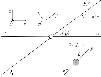
Figure 1.9 A schematic of the coordinate systems used in the analysis of

KY photoproduction. Two different coordinate systems are

used: the unprimed and primed. The unprimed coordinate

sys-tem has its z–axis aligned with the incoming photon

momen-tum, ˆz = ˆpγ. The y–axis, ˆy = ˆz×pˆK. The x–axis, ˆx = ˆy×zˆ.

In the primed coordinate system, thez0–axis is along the kaon

momentum ˆz= ˆpK. The y0–axis is defined as ˆy0 = ˆz0×pˆγ. The

x0–axis is thus ˆx0 _{= ˆ}_y0 _×_z_ˆ0_{. For both coordinate systems, the}

reaction occurs in the x–z (x0–z0) plane. . . 15

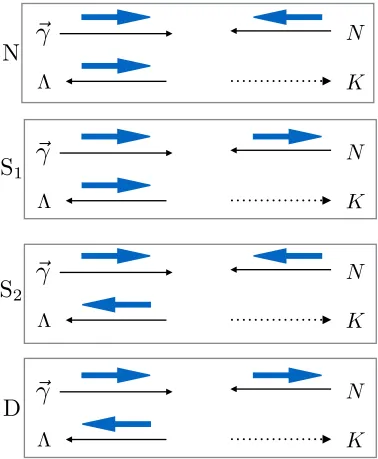
Figure 1.10 The four helicity amplitudes in pseudoscalar meson

photopro-duction. The label "N" corresponds to the no–spin flip

ampli-tude, "S1(2)" corresponds to the single spin flip amplitudes, and

"D" corresponds to the double spin flip amplitude. . . 19

Figure 1.11 Three mechanisms to photoproduce KY. A resonance, N∗ is

created in thes channel that then decays into the KY. In the

t (u) channel, a K∗ (Y∗) is exchanged. . . 21

Figure 1.12 Two example fits ((a) and (b)) of the cross section ofγp→K+_Λ

from the Bonn–Gatchina group. The solid curves are the

re-sults of the fits, the dashed lines areP13(N(1900)3₂, N(1720)3₂)

contributions, the dotted lines are S11 (N(153501₂, N(1650)1₂)

contributions, and the dashed–dotted line is thet–channel

con-tribution. This image was taken from Reference [8] . . . 22

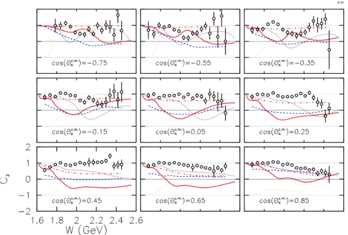
Figure 1.13 Cz as a function of the center–of–mass energy W for different

cosθCM

K bins. The open circles are the experimental values for

the observable. The different colored curves represent predic-tions from different hadronic models. The image was taken from

(15)

Figure 1.14 Ox as a function of the center–of–mass energy W for different

cosθCM

K bins. The black circles are the experimental values

for the observable. The red curves are predictions from ANL– Osaka [31], green colored curves from the 2014 Bonn–Gatchina group[29], and the blue curves are ref–fits including the present

data with and an additionalN∗3₂+andN∗5₂+added. This image

was taken from Reference [46] . . . 24

Figure 1.15 The red and black data points on both histograms are the two sets of Jefferson Lab data. The left panel shows the data points with Kaon–MAID models with two different sets of input pa-rameters [33]. The right panel shows the cross sections from

K+_{Λ superimposed on top of the} _K0_{Λ data. Also drawn are}

two different PWA solutions from the Bonn–Gatchina group

for the K0Λ (green lines) and the 2014 solution for the K+Λ

data.This image was taken from [18]. . . 26

Figure 2.1 A schematic of CEBAF at the time the experiment took place.

One can see the 0.6 GeV linacs, the recirculating arcs, and the three experimental halls (Hall A, Hall B, and Hall C) at the

time of the experiment. This figure is taken from Reference [39] . 30

Figure 2.2 A schematic of the Hall–B beam line during the g13a

experi-ment. From left to right, along the beam direction one can see the Møller polarimeter, the radiator and the tagging spectrom-eter, the subsystems of the CLAS detector, the photon profile monitor, and the total absorption counter. Not shown is the photon collimator placed between the tagger and the CLAS.

Figure is from [39]. . . 30

Figure 2.3 A schematic of the photon tagger in Hall B. Electrons,

inci-dent from the left, that interacted with the radiator produced bremsstrahlung photons that continued in the original direc-tion of the incident electron beam. The electrons were bent by a dipole magnet at different angles based on their energy. A two-plane hodoscope detected these electrons, which allowed for energy and time measurements. This figure is taken from

Reference [53] . . . 33

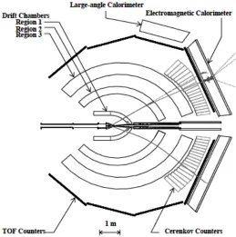
Figure 2.4 A schematic of the CLAS detector. Drift Chambers measure

particles’ trajectories and TOF Counters measure the time of

(16)

Figure 2.5 A cross section of the magnetic field vectors for the CLAS toroidal field in a plane perpendicular to the beam line. The locations of the coils are indicated by thick solid lines. One can see the field distortions in the areas close to the coils. This

image is taken from Reference [39]. . . 35

Figure 2.6 A schematic of the start counter in CLAS. One can see the six

identical sectors of four scintillators per sector. This image was

taken from Reference [51]. . . 36

Figure 2.7 A schematic of CLAS detector as seen from the perspective of

looking down the beam line. One can see how the CLAS is di-vided into six sectors by the main torus coils. The three regions of drift chambers are situated between these coils and track the trajectories of charged particles as they travel through the de-tector. The mini–torus is a magnet used in electro-production experiments. It was not used in g13, where the start counter

was placed in its location. This image is taken from Reference [39]. 37

Figure 2.8 One sector of the time–of–flight system. Each sector of 56

pad-dles was positioned such that each paddle covers different polar

angle. This image is taken from Reference [52]. . . 39

Figure 3.1 ∆β as a function of momentum for protons as measured by the

CLAS, i.e. without any corrections applied. One clearly sees

that true protons yield a distribution centered around ∆β of

zero. The leaf–like structures that seem to originate from the proton distribution at low momenta and to follow a different trend at higher momenta are due to true protons that have incorrect timing. A lot of background events, such as pions and kaons are not seen in this figure. This is due to the fact that

extra selection cuts, such as photon selection, K0 _{selection, Λ}

selection, and missing mass cuts (all to be discussed) have been applied to the event sample in order to reduce the uncertainty of the proton PID cuts. The vertical black lines represent the

(17)

Figure 3.2 Projections and the Gaussian fit of the proton ∆βfor the 10 mo-mentum bins shown in Fig. 3.1. Even though extra cuts have been applied to the event sample to remove accidental back-ground, some background events remain. Those contribute to the non–Gaussian tails of the projections. In order to determine the widths of those nearly–Gaussian distributions by fits to a Gaussian function in a consistent manner, the fit ranges were

set to be [-0.025,0.025]. . . 42

Figure 3.3 Final ∆β cuts for the proton (red line). The red data points

represent the ±3σ points determined from the Gaussian fits in

Fig. 3.2. These points were then fit with a 4thorder polynomial

to determine the ∆β cut. . . 43

Figure 3.4 ∆β vs. pdistribution for theπ+_{. The red data points represent}

the±3σ points determined from the Gaussian fits to the

differ-ent momdiffer-entum bins. These points were then fit with a 4th_order

polynomial to determine the final ∆β cut (red line). The small

structure at low momenta and positive delta beta is most likely

due to trueπ+_{s that decay before they reach the time–of–flight}

detector. The daughter muon moves along a path that is

suffi-ciently close to the trajectory of the parent π+ so that a single

track is reconstructed. The momentum of the track however is

different from the momentum of the parentπ+_{. . . .} ₄₃

Figure 3.5 ∆β vs. p distribution for the π−. The red data points

repre-sent the ±3σ points determined from the Gaussian fits to the

different momentum bins. These points were then fit with a

4th _{order polynomial to determine the final ∆}_β _{cut (red line).}

The small structures at low momenta and positive delta beta

are most likely due to true π−s that decay before they reach

the time–of–flight detector. The daughter muon moves along a path that is sufficiently close to the trajectory of the parent

π− so that a single track is reconstructed. The momentum of

the track however is different from the momentum of the parent

π−. This effect is typically observed for out bending pions, i.e.

π− in g13a. . . 44

Figure 3.6 The z component of the production vertex. Events were kept

if they originated within the target. . . 45

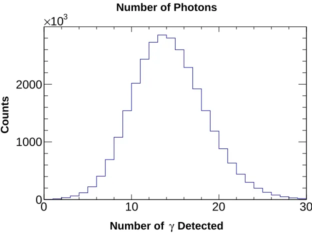
Figure 3.7 Number of photons detected per event in g13a. The photon

(18)

Figure 3.8 Coincidence time for all particles and the fastest particle in CLAS. The smaller peaks that are separated by 2 ns show the

structure of different electron beam bunches. . . 47

Figure 3.9 Number of photons yielding a coincidence time within ±1 ns

per event. Events with 2 or more photons within the time-coincidence cut were removed from further analysis since there is no reliable mechanism to identify which amongst them was

most likely the "good" photon. . . 48

Figure 3.10 The DOCA method used to reconstruct the decay vertices of

the K0 _{and Λ. The DOCA occurs along the line perpendicular}

to each track (solid black line). The reconstructed decay vertex,

represented by the ?, is the bisector of the DOCA line. . . 50

Figure 3.11 M(π+π−) as a function of M(pπ−). The peak containing to

K0_{Λ events sits on top of a broad background. The background}

is mostly due to γd → pπ+_π−_π−_X _{events uncorrelated with}

K0Λ production. . . 51

Figure 3.12 M(π+_π−_{) distribution after all previous cuts are applied. The}

peak was fit with a Gaussian and the vertical lines represent

±4σ cuts used to selectK0 _{events. . . .} ₅₂

Figure 3.13 M(pπ−) distribution after all previous cuts, includingK0

selec-tion, were applied. The peak was fit with a Gaussian and the

solid vertical lines represent ±4σ cuts used to select Λ events. . . 53

Figure 3.14 Distribution of K0_Λ_X _{events (where} _X ₌ _p_{) over the}

specta-tor momentum, |p~X|. Events below 0.2 GeV/c form a sample

dominated by the quasi–free reaction. . . 54

Figure 4.1 MK0_X as a function ofM_X. Visually, the main peak centered at

MX =Mp and MK0_X =M_Λ contains the signal events. Higher

mass channels in MX and MK0_X contain background channels

such as K0_Σ0_, _K0_Σ∗0_{, and} _K?_{(892)Λ photoproduction. The}

arrows point to the general area of these different channels. . . 57

Figure 4.2 Fitting procedure and momentum correction example for the

proton. The data were binned in different z–vertex, φ, and θ

bins. For each bin, the ∆p vs. |~p| distribution was divided into

5 |~p| bins. For each p bin, ∆p was fit with a Gaussian. The

means for the momentum bins were then fit with an exponential

(19)

Figure 4.3 Momentum of theπ+ _{for the simulation scaled (red) to the data}

(blue) for 100–MeV wide Eγ bins. . . 61

Figure 4.4 Momentum of theπ−from the Λ for the simulation scaled (red)

to the data (blue) for 100–MeV wideEγ bins. . . 62

Figure 4.5 Momentum of the proton for the simulation scaled (red) to the

data (blue) for 100–MeV wide Eγ bins. . . 63

Figure 4.6 Momentum of the π− from the K0 for the simulation scaled

(red) to the data (blue) for 100–MeV wideEγ bins. . . 63

Figure 4.7 cosθ_KCM0 for theK0Λ simulation scaled (red) to the data (blue)

for 100–MeV wideEγ bins. . . 64

Figure 4.8 The missing–mass, MX, of γd → K0Λ(X) with the selection

cuts described in Chapter 3 integrated over all kinematics. . . 67

Figure 4.9 A visualization of Eqs. 4.10, 4.11, 4.12, and 4.13 on MX. In

a given region ofMX, shown as the black lines at 0.9 and 0.98

GeV/c2_{, the total observable is extracted. . . .} ₆₉

Figure 4.10 An example fit and scaling of the non–resonant, unpolarized

γd → pπ+_π−_π−₍_p_{) simulated background to the data using}

Equation 4.23. A double Gaussian is used to describe the signal

and a parameter from the fit,A3, is used to scale the unpolarized

background (magenta) to the data. . . 71

Figure 4.11 Example fits and scaling of the non–resonant, unpolarized

sim-ulation to the data for oneEγ bin. The red line is the total fit

to the data and the magenta histogram is the pπ+π−π− non–

resonant background scaled using A3 from Equation 4.23. . . 72

Figure 4.12 The χ2/NDF and scale factor (A3 in Eq. 4.23) for all the fits.

Theχ2_{/NDF is used as a check on the goodness of fit, while}_A

3

provides the scale factor for thepπ+_π−_π− _{non–resonant background. 73}

Figure 4.13 Total fit using Equation 4.24 (red line) to the data (blue points)

and scaling toMX integrated over all kinematics. The magenta

histogram is the scaled non–resonant background, the green

histogram is the scaledK0_Σ0 _{distribution, and the black}

(20)

Figure 4.14 Fits and scaling to MX for 2.1 < Eγ < 2.2 GeV. The red line

is the total fit to the data, the red histogram is the scaled

pπ−π+_π− _{distribution, the green histogram is the scaled} _K0_Σ0

distribution, and the black and violet histograms are the scaled higher mass channels. The black lines are drawn to show the

separation of the Regions. . . 76

Figure 4.15 The χ2_{/NDF and scale factor (}_A

4 in Eq. 4.24) for all the fits.

Generally speaking, theχ2_{/NDF from these fits are larger than}

those seen in theM(pπ−) fits. This is likely due to the fact that

there are significantly more fit parameters in Equation 4.24 than there are in Equation 4.23. The small value for the scale factor suggests that there is enough statistics in the simulations to

accurately scale the background. . . 77

Figure 5.1 (Top) The instrumental asymmetry as a function of run

num-ber for pX <0.2 GeV/cintegrated over all kinematic variables.

(Bottom) The pull distribution fit with a Gaussian. The results suggest that there is no time–dependent instrumental

asymme-try in the g13a data set. . . 81

Figure 5.2 A as a function of φ (top row) for the pion (left) and

pro-ton (right) with their corresponding pull distributions (bottom row). The fits to the pull distributions show no significant

bi-ases or unaccounted for uncertainties in the data. . . 84

Figure 5.3 Relative pull distributions for Cx (left), Cz (middle), and P

(right) from the proton selection. From the parameters, no

significant systematic uncertainties are seen in Cx, Cz, or P. . . . 86

(right) from the π+ _{selection. From the parameters, no}

signifi-cant systematic uncertainties are seen in Cx, Cz, or P. . . 87

(right) from the π− selection. From the parameters, no

signif-icant biases or systematic uncertainties are seen in Cx, Cz, or

P. . . 89

Figure 5.6 M(pπ−) distribution with lines representing ±4σ (black) and

±0.7σ (red), where σ is determined from the fit in Fig. 3.13.

To investigate the systematic uncertainties, a relative pull

(21)

Figure 5.7 Relative pull distributions for the two different regions inM(pπ−).

From the parameters, no significant biases are seen forCxorCz.

The mean for P is more than 3σ from 0, which suggests there

may be some systematic uncertainty caused by theM(pπ−)

se-lection. . . 91

Figure 5.8 Differences between the observables for the two different regions

inM(pπ−). When fit with a Gaussian, the means of Cx andCz

are consistent with 0. The mean of P is significantly different

than 0. . . 93

Figure 5.9 Distributions ofσ2

sys for the observables. The parameters of the

fit suggest there are no significant systematic uncertainties. . . 94

Figure 5.10 M(π+_π−_{) distribution with lines representing}_±4_σ _{(black) and}

±0.7σ (red), where σ is determined from the fit shown in Fig.

3.12. The systematic uncertainty related to theM(π+_π−₎

selec-tion is studied through relative pull distribuselec-tions and differences

in observables between the two regions. . . 96

(right) from the M(π+π−) selection. From the fit parameters,

no significant biases are seen. . . 97

Figure 5.12 Distribution of φ as a function of θ for a π− without (left)

and with (right) fiducial cuts applied. The fiducial cuts reject

particles that travel close to the sector edges. . . 98

Figure 5.13 Distribution of φ as a function of θ for the events removed by

the fiducial cuts for the p (top left), π+ _{(top right), and} _π−_s

(bottom row). . . 99

Figure 5.14 Relative pull-distributions for Cx (left), Cz (middle), and P

(right) from applying the fiducial cuts. From the parameters,

no significant systematic uncertainties are seen inCxorCz. The

mean ofP is significantly different from 0, suggesting there may

be some systematic uncertainty. . . 100

Figure 5.15 Differences between the observables when using “good” and

“bad” samples. The means for Cx and Cz are consistent with

0, whereas the mean forP is ≈4σµ from 0. . . 101

Figure 5.16 Distribution of σ_sys2 for Cx (left), Cz (middle), and P (right) .

(22)

Figure 5.17 The correlation between "good" (estimated from events that pass the fiducial cuts) and "bad" (estimated from events where at least one particle fails the fiducial cut) observables. The parameters of the fits suggest there are no significant systematic

biases forCx andCz. Since the Y-intercept forP is inconsistent

with 0, while the slope is consistent with 1, the systematic bias

inP is a bias with the form µ+δ. . . 103

Figure 5.18 Event distribution over the magnitude of spectator momentum,

pX. The red line divides pX into two regions, Region 1 and

Region 2. . . 104

(right) from the pX selection. From the parameters, no

signifi-cant systematic uncertainties are seen in Cx, Cz, or P. . . 105

Figure 5.20 Differences between the observables for the two different regions

inpX. When fit with a Gaussian, the means of the differences

are consistent with 0. . . 106

Figure 5.21 Distribution of σ2

sys for Cx (left), Cz (middle), and P (right) .

The means of the fits suggest there are no significant systematic

uncertainties. . . 107

Figure 5.22 Fits to MX for different cosθCM_K0 in the highest Eγ bin. There

are multiple cosθCM

K0 in this Eγ bin where the fits are not able

to describe the data. . . 108

Figure 5.23 Generator flowchart for studying systematic effects originating

from the maximum likelihood extraction method. . . 109

Figure 5.24 Pull distributions for Cx =Cz =P = 0 for 1,000 experiments,

with 10,000 generated events in each experiment, fit with a Gaussian. The means and the widths of the pull distributions

do not significantly differ from 0 and 1, respectively. . . 111

Figure 5.25 Observable differences for Cx = Cz = P = 0 for 1,000

experi-ments with 10,000 generated events fit with a Gaussian. . . 111

Figure 5.26 Pull distributions forCx= 0.2,Cz = 0.8, andP = 0.5 for 1,000

experiments with 10,000 generated events fit with a Gaussian. The means and the widths of the distributions do not

(23)

Figure 5.27 Observable differences for Cx = 0.2, Cz = 0.8, P = 0.5 for

1,000 experiments with 10,000 generated events fit with a

Gaus-sian. . . 113

Figure 5.28 Pull distributions for random Cx, Cz, and P for 1,000

experi-ments with 10,000 generated events fit with a Gaussian. . . 114

Figure 5.29 Correlation plot for random Cx, Cz, and P for 1,000

exper-iments, with 10,000 generated events in each experiment, fit

with a Gaussian. . . 115

Figure 5.30 Calculated acceptance from Equation 5.8 for eachEγand cosθKCM0

bin. . . 116

Figure 5.31 Example of A(cosθy,cosθz) for 1.5 < Eγ < 1.6 GeV and 11

cosθ_KCM0 bins. We observe that the CLAS acceptance is non–

uniform over the proton direction cosines. . . 117

Figure 5.32 Pull distributions for random Cx, Cz, and P for 1,000

Figure 5.33 Correlation plots for random Cx, Cz, and P for 1,000

Figure 5.34 Distributions of the difference between the extracted and the

true values for random Cx, Cz, and P for 1,000 experiments,

with 500,000 generated events in each experiment, fit with a

Gaussian. Cx and Cz have means (µ) consistent with 0 and

have no bias. P has µ = 0.026±0.001 which shows that the

extracted values ofP are biased. . . 119

Figure 5.35 ∆Obs as a function of the true observable for random Cx, Cz,

and P for 1,000 experiments with 500,000 generated events fit

with a Gaussian. The slope for each,Cx, Cz,andP is consistent

with 0. This means any shift in ∆Obs does not depend on the

value of the observable. . . 120

Figure 5.36 Correlation plot for random Cx, Cz, and P for 1,000

exper-iments with 500,000 generated events in each experiment fit

with a Gaussian. Cx and Cz have slopes and Y–intercepts

con-sistent with 1 and 0, respectively. The constant for P is not

(24)

Figure 5.37 Normalized difference between the 0.97 and 0.99 GeV/c2

selec-tion cut for region 1. At low energies, there is a small difference between the number of events in region 1. At higher energies,

there are≈20% more events in region 1 for theMX separation

of 0.99 GeV/c2_{. . . .} ₁₂₃

Figure 5.38 Difference in observables when changing the MX range in the

background subtraction method for region 1. The observables

are fit with a Gaussian and the mean,µ, plus width, σ, added

in quadrature, are reported as systematic uncertainties. . . 124

Figure 5.39 ∆Cz when changing the ratios in the background subtraction

method for each kinematic bin. . . 125

Figure 5.40 Relative difference for Cx, Cz, and P for 25 and 50 MX bins.

All observables have relative differences of 10−3 _{or less and it}

can be concluded that decreasing the number ofMX bins from

50 to 25 does not cause any systematic error in the observ-ables. The standard deviation of each distribution quantifies

the systematic uncertainty of the corresponding observable. . . 126

Figure 5.41 Relative difference for Cx, Cz, and P for 75 MX bins. All

ob-servables have relative differences of 10−3 _{or less and it can be}

concluded that increasing the number of MX bins from 50 to

75 does not cause any systematic error in the observables. The standard deviation of each distribution quantifies the

system-atic uncertainty of the corresponding observable. . . 127

Figure 6.1 Eγ as a function of cosθKCM0 after selection cuts on M(pπ−),

M(π+_π−_{), and} _p

X < 0.2 GeV/c. The black lines represent

the edges of the different kinematic bins. The background sub-traction and observable exsub-traction method were done for each

kinematic bin. . . 131

Figure 6.2 The ratio of photon polarization to the electron polarization

as a function of the ratio of photon energy to electron energy. The photon polarization was calculated using Eq. 5.10. The electron polarization was measured by the Møller polarimeter

in Hall B. . . 133

Figure 6.3 Cx as a function of cosθCMK0 for the 16 different Eγ bins. The

red and blue curves are the two Bonn–Gatchina soultions from

(25)

Figure 6.4 Cz as a function of cosθ_KCM0 for the 16 different Eγ bins. The

red and blue curves are the two Bonn–Gatchina soultions from

the cross–sections projected (not fit) ontoCz. . . 134

Figure 6.5 P as a function of cosθCM

K0 for the 16 differentEγ bins. The red

and blue curves are the two Bonn–Gatchina soultions from the

cross–sections projected (not fit) ontoP. . . 135

Figure 6.6 R=qC2

x +Cz2+P2as a function of cosθCMK0 for the 16 different

Eγ bins. The blue line is a constant fit to R for each Eγ bin.

The width of the line is the uncertainty of the fit. . . 136

Figure 6.7 Cx as a function of W =

q

m2

n+ 2mnEγ for the 14 different

cosθ_KCM0 bins. . . 137

Figure 6.8 Cz as a function of W =

q

m2

Figure 6.9 P as a function of W = qm2

Figure 6.10 Cx as a function of cosθKCM0 for the 16 different Eγ bins for

the primed coordinate system. The dashed lines correspond to Kaon–MAID solutions [33] for the observable and the solid line are model predictions from A. Waluyo [55]. The red and blue lines correspond to predictions with and without an extra

N(1900)3₂− state, respectively. . . 139

Figure 6.11 Cz as a function of cosθCM_K0 for the 16 different Eγ bins for

the primed coordinate system. The dashed lines correspond to Kaon–MAID models [33] for the observable and the solid line are model predictions from A. Waluyo [55]. The red and

blue lines are predictions with and without an extraN(1900)3₂−

state, respectively. . . 140

Figure 6.12 P as a function of cosθ_KCM0 for the 16 different Eγ bins for the

primed coordinate system. The dashed lines are Kaon–MAID models [33] for the observable and the solid line are model pre-dictions from A. Waluyo [55]. The red and blue lines are

(26)

Figure 6.13 A comparison of Cx for γd→ K0Λ(p) (black) and γp→ K+Λ

(blue). Each cosθCM

K0 bin is drawn at the bin centroid as

op-posed to the bin average to match the free proton data. . . 142

Figure 6.14 A comparison of Cz for γd → K0Λ(p) (black) and γp → K+Λ

(blue). Each cosθCM_K0 bin is drawn at the bin centroid as

op-posed to the bin average to match the free proton data. . . 142

Figure 6.15 Cx (blue), Cz (red), and P (green), integrated over all Eγ and

cosθ_KCM0 , as a function of the neutron momentum. Each

observ-able is fit with a first order polynomial. . . 144

Figure 6.16 Cx for 8Eγ as a function of the neutron momentum integrated

over all cosθCM

K0 . Each bin is fit with a line in the quasi–free

region (|pn|<0.2 GeV/c). . . 145

Figure 6.17 Cz for 8 Eγ as a function of the neutron momentum integrated

over all cosθCM_K0 . Each bin is fit with a first order polynomial in

the quasi–free region (|pn|<0.2 GeV/c). The numbers in each

panel denote the % difference between the average value of the observable within the quasi–free range of neutron momentum

and the extrapolated value to a neutron momentum of zero. . . . 145

Figure 6.18 P for 8Eγ as a function of the neutron momentum integrated

over all cosθ_KCM0 . Each bin is fit with a first order polynomial

(27)

Chapter 1 Introduction

Visible matter is made up of atoms, which consist of particles called protons, neutrons,

and electrons. Protons and neutrons (known as nucleons) bind together to form the

nucleus where nearly all the mass of the atom is concentrated. The nucleons are made

up of even smaller particles, known as quarks and gluons. A simplistic picture of a

nucleon consists of three quarks that interact to give a nucleon its physical properties.

Along this line of thinking, summing the three quark masses (the gluons are massless)

should lead to the mass of the nucleon. However, this summation only accounts for

≈2% of the nucleon mass [47]. The rest of this mass emanates from the interactions

between quarks and gluons.

One of the main goals of nuclear physics is to understand how the nucleons come

into being and the fundamental interactions that lead to this. The Standard Model is

a theory that aims to describe the interactions between all elementary particles, such

as quarks, and the forces that mediate these interactions [27]. While there are still

questions that remain in the Standard Model, theories like Quantum Electrodynamics

(QED) and Quantum Chromodynamics (QCD) have done a fantastic job describing

the interactions that occur between elementary particles. QED describes how light

and matter interact with each other and served as a base for developing QCD. QCD

is the theory that currently describes the interactions between quarks and gluons.

It is able to describe how they interact at small distances, but not how they bind

(28)

1.1 Standard Model

The Standard Model states that matter consist of three elementary, or

fundamen-tal, types of particles: quarks, leptons, and mediators [27]. It describes how these

elementary particles interact with each other within three fundamental forces: the

strong, weak, and electromagentic. The only fundamental force the Standard Model

does not describe is the gravitational force.

Figure 1.1 lists the elementary particles in the Standard Model [2]. Matter is

broken down into two subgroups: fermions and bosons. The fermions have half–

F

O

R

C

E

C

A

R

IER

S

L

EPT

O

N

S

QUARKS

Figure 1.1: Elementary particles in the Standard Model that describes the fundamen-tal interactions between elementary particles. Matter consists of three elementary, or fundamental, types of particles: quarks, leptons, and force carriers. This image was taken from Reference [2].

integer spin and consist of six quarks and six leptons. The quarks and leptons are

split into three generations of matter based off the mass of the particles. The first

and lightest generation contains the up quark, down quark, electron, and electron

(29)

generation contains the charm quark, strange quark, muon, and muon neutrino. The

third and heaviest generation contains the top quark, bottom quark, tau, and tau

neutrino. The gauge bosons have integer spin and mediate the strong, weak, and

electromagnetic forces.

The leptons are classified according to their charge, electron number, muon

num-ber, and tau number. There are also 6 antileptons whose internal quantum numbers

have opposite sign, totaling 12 particles. Leptons can only interact via the

electro-magnetic, weak, and gravitational forces. Like the leptons, the quarks are classified

according to their charge and flavor. Additionally, there are six antiquarks that have

opposite charge and flavor. Quarks contain an additional property known as color

charge. With 3 color charges (red, green, blue) and 12 particles, there are a total of

36 quarks.

The gauge bosons mediate 3 of the 4 fundamental forces. The gluon mediates

the strong force, the photon the electromagnetic, and the W and Z bosons the weak.

The massless gluon can only interact with themselves or quarks as they are the

only particles that carry color charge. Photons, which are also massless, can only

interact with particles that carry electromagnetic charge. The massive W and Z

bosons mediate the weak interaction. Both leptons and quarks participate in the

weak interaction

The Higgs Boson, predicted in 1964, was the last particle predicted by the

Stan-dard Model to be discovered [30]. A particle consistent with the Higgs Boson was

discovered by the ATLAS and CMS Collaborations in 2012 [3, 16].

1.2 Quantum Chromodynamics

Quantum chromodynamics (QCD) is the theory of the strong interaction and it

de-scribes the interactions between quarks and gluons. As mentioned above, the three

(30)

b, there are 3 anticolor charges: antired (¯r), antigreen (¯g), and antiblue (¯b). Quarks

carry a single color charge, while gluons carry both a color and anticolor charge. Color

charge is analogous to the electric charge in Quantum Electrodynamics (QED).

How-ever, photons do not carry electromagnetic charge while gluons carry color charge.

The strength of the interaction in QCD is given by the strong coupling constant,

αS [27]. When αS is much smaller than 1, the interaction is weak and perturbation

theory can be used to solve QCD. WhenαS is on the order of 1, then the interaction

is strongly coupled and can not be solved using perturbation theory. For comparison,

the coupling constant in QED, the fine structure constant, α = 1

137 << 1, meaning

perturbation theory can be used to solve QED. In QCD,αSdepends on the separation

distance between the interacting particles [27]. At short interaction distances (high

energies), αS is small and approaches zero when the interaction distance approaches

zero. This phenomenon is known as asymptotic freedom, discovered independently by

Wilczeck and Gross [28] and Politzer[48]. At large interaction distances (low energies),

αS is on the order of 1, which leads to the phenomenon of color confinement. Color

confinement prohibits an individual color–charged particle (quark or gluon) from

being isolated as free particles. If one tries to separate one quark from another

quark, it becomes more energetically favorable to create a new pair of quarks.

The fundamental degrees of freedom for QCD are the quarks and gluons. Since

color confinement prevents quarks and gluons from being isolated, the fundamental

degrees of freedom of QCD can not be directly studied. One way to study QCD in

the confinement regime is to study the properties of hadrons, which are composite

particles made up of quarks and gluons that are bound by the strong force. Inside

of hadrons, like the proton and neutron, is what is referred to as a sea of quarks and

gluons. The particles in the sea are constantly interacting with each other and with

the valence quarks. Gluons spontaneously split into quark–antiquark pairs, which

(31)

and sea quarks that gives rise to the nucleon mass. A valence quark immersed in a

cloud of sea quarks and gluons has a large mass, when compared to a bare quark,

and is referred to as a constituent quark. Since confinement prevents the study of

the fundamental degrees of freedom in QCD at large distances, the effective degrees

of freedom, which are the constituent quarks and gluons, need to be studied.

1.2.1 Hadrons

Hadrons are divided into two subgroups: baryons and mesons. Baryons are particles

that consist of three constituent quarks (qqq), while mesons are particles that are

made up of a constituent quark–antiquark pair (qq¯). In addition to being made up

of a different number of constituent quarks, baryons have half–integer spin and are

fermions while the mesons have integer spin and are bosons.

Prior to the discovery of the strange quark, SU(2) symmetry was successful in

explaining the difference between the u and d quarks. Here, isospin is the

symme-try that explains the difference between the observed properties of the discovered

hadrons. As more hadrons were discovered, SU(2) symmetry could not explain the

long lifetimes of some of these newer particle states [25]. This led to describing the

hadrons with SU(3) symmetry, where 3 represents the three flavors of light quarks:

u, d, and s.

Figure 1.2 shows the pseudoscalar meson nonet, introduced by Murray Gell–Mann

in the Eightfold Way [25]. The Eightfold Way is a scheme used to order and classify

hadrons according to their strangeness and charge. The mesons are ordered via

properties determined from their constituent quarks. Only three quarks– (u, d, s)

were included by Gell–Mann when he proposed the Eightfold Way. Figure 1.3 shows

the corresponding baryon octet from the Eightfold Way. In Gell–Mann’s SU(3) group,

all three quarks have the same masses. However, it is known that the quarks do not

(32)

Figure 1.2: The meson nonet. Particles with the same strangeness are arranged horizontally and particles with the same charge are arranged diagonally. This image is taken from Reference [1].



T

TT

T





r

rr

r

n

p

⌅

0

⌃

+

⌃

0

⇤

s

= 0

s

=

1 s

=

2 q

=

1 q

= 0

q

= 1

Figure 1.3: The baryon octet. Particles with the same strangeness are arranged

horizontally and particles with the same charge are arranged diagonally. Figure

adapted from Reference [57].

having different masses. In addition to organizing the already discovered particles,

(33)

1.3 Baryon Spectroscopy

One way to study the effective degrees of freedom of QCD is to measure the excited

states of hadrons. In the early 1900’s, atomic spectroscopy was used to measure

excited states of the atom. In atomic spectroscopy, energy is absorbed by an atom,

causing an electron to move to a higher energy state. Some time later, the atom

will de–excite and typically emit a photon that corresponds to the energy between

the initial and final states. By measuring these emitted photons, the atomic orbital

structure was mapped out, leading to the modern understanding of the atom.

Hadron spectroscopy works in a similar manner. Adding energy to a hadron can

cause the constituent quarks to reform and the hadron will enter an excited state, also

called a resonance. Some time later, this excited state will decay by emitting some

combination of hadrons and photons. Ultimately, the goal of baryon spectroscopy is

to provide information about the effective degrees of freedom in the non–perturbative

regime of QCD. The rest of this work will focus on baryon spectroscopy, specifically

the excitation of nucleons.

The Particle Data Group (PDG) lists 15 established excited nucleon (N∗) states

below 3000 MeV [47]. The PDG assigns a * to **** rating to excited states. * means

evidence for the state is poor, ** evidence is fair, *** existence is very likely but

more information is needed, and **** ratiing means that the existence is certain and

the properties of the state have been explored. To move from *** to ****, the N∗

needs to be seen across multiple decay modes. Table 1.1 lists the overall status of

the N∗s and the rating for each decay channel. All states below 1800 MeV have an

overall rating of *** or better and were predominately seen in either N∗ → N π or

N∗ →N γ. Above 1800 MeV, there are many states that only have a ** or * rating. It

has been predicted that many of these higher–mass states have significant branching

(34)

Table 1.1: The status of the N∗s. A * means evidence for the state is poor, ** evidence is fair, *** evidence is very likely but more information is needed, and **** means the evidence is certain and the properties of the state have been explored. The table is adapted from the PDG [47].

Particle JP _overall _{N γ} _{N π} _{N η} _{N σ} _{N ω} _Λ_K _Σ_K _{N ρ} _∆_π

N1/2+ _****

N(1440)1/2+ _**** _**** _**** _*** _* _***

N(1520)3/2− **** **** **** *** *** ***

N(1535)1/2− **** **** **** **** ** *

N(1650)1/2− **** **** **** *** *** ** ** ***

N(1675)5/2− _**** _**** _**** _* _* _* _***

N(1680)5/2+ _**** _**** _**** _* _** _*** _***

N(1700)3/2− *** ** *** * * * * ***

N(1710)1/2+ _**** _**** _**** _*** _** _**** _** _* _**

N(1720)3/2+ **** **** **** *** ** ** ** *

N(1860)5/2+ _** _** _* _*

N(1875)3/2− *** *** * ** *** ** ***

N(1880)1/2+ _** _* _* _** _*

N(1895)1/2− ** ** * ** ** *

N(1900)3/2+ _*** _*** _** _** _** _*** _** _* _**

N(1990)7/2+ _** _** _** _*

N(2000)5/2+ _** _** _* _** _** _* _**

N(2040)3/2+ * *

N(2060)5/2− ** ** ** * **

N(2100)1/2+ _* _*

N(2120)3/2− _** _** _** _* _*

N(2190)7/2− **** *** **** * ** *

N(2220)9/2+ _**** _****

N(2250)9/2− **** ****

N(2300)1/2+ ** **

N(2570)5/2− ** **

N(2600)11/2− *** ***

N(2700)13/2+ _** _**

The cross section of a resonance produced by a +b → N∗ has the shape of a

Breit–Wigner distribution,

σ(s) = σmax

m2₀Γ2

(s−m2

0)2+m20Γ2

, (1.1)

wheres= (˜pa+ ˜pb)2 is the center–of–mass energy squared, m0 is the mass of the

(35)

cross section that contains information about the spin of the incoming particles, a

and b, as well as the angular momentum of the N∗. The lifetime of the resonance is

inversely proportional to Γ. A short lifetime corresponds to a large width, whereas a

long lifetime corresponds to a small width. Generally speaking, the typical lifetime

of a nucleon or baryon resonance is 10−23_{s, meaning the widths of the resonances are}

quite large (when compared to the excited states of a Hydrogen atom). This results

in a spectrum of broad and overlapping resonances when looking at the energy

de-pendence of the cross section of a +b → N∗. Therefore, in depth analyses, both

experimental and theoretical, need to be performed to extract the masses, spins, and

parities of the N∗s. Experimentalists collect data and extract observables and cross

sections by measuring the decay products of the N∗s. Theorists then use these

ob-servables to extract information about the states using partial wave analyses (PWA).

PWAs break the cross section into a series of partial waves and relate each partial–

wave to a corresponding angular momentum. Quark models and lattice QCD are also

used by theorists to predict the resonant spectrum.

1.3.1 Constituent Quark Models

Different models have been developed in an attempt to understand the interactions

of quarks and gluons inside of baryons. These models have different effective degrees

of freedom, symmetries, and dynamics that lead to a different number of predicted

excited states. Figure 1.4 shows the most general and simplest quark model, known

as constituent quark models. These postulate a baryon consisting of three valence

quarks. The baryon wave function, ψ, is given by,

ψ =ψcolorψspinψspaceψf lavor, (1.2)

whereψcolor is the color component,ψspin is the spin component, ψspace is the spatial

(36)

Figure 1.4: A simple schematic of the quark arrangement in constituent quark models. Each of the three quarks interacts equally with each other.

it is known that all hadrons must be in a colorless (a color singlet) antisymmetric

state. Since ψ has to be antisymmetric and ψcolor is antisymmetric for all baryons,

then ψspinψspaceψf lavor must be symmetric, as in the case of the ∆++

The full spectrum of baryons can be obtained by solving the wave equation of three

particles moving in a potential,H|ψi=E|ψi. The earliest constituent quark models

(CQMs) treated the three quark interaction as an harmonic oscillator potential [22],

H =X

j

p2_j

2M +

1

2M ω

2X

i<j

(ri−rj)2, (1.3)

wherepj is the quark momentum andri−rj is the distance of separation between two

non–identical quarks. More recent CQMs, like those of Capstick and Isgur treat the

potential between quarks as arising from the exchange of gluons [14]. Depending on

the model, the forms of these potentials can change. A review of the different quark

models and their predictions for the spectrum of baryons can be found in Reference

[13].

Generally speaking, CQMs predict more excited states than have been

(37)

CQMs having the wrong degrees of freedom– that is more degrees of freedom than

actually present inside of baryons. On the other hand, there may not be enough data

available to observe these "missing" baryons. Up until the 2000’s, data predominately

consisted of measuring resonant decays into nucleon–pion final states. Capstick and

Roberts suggested that several of these "missing" states were likely to be observed in

channels decaying into strange particles, such asKΛ [15].

Figure 1.5 shows the predicted excited nucleon spectrum for N∗ decays into N γ

(white), N π(light grey), and KΛ(black) [15]. The Y–axis is the mass of the state

Figure 1.5: Predicted N∗ decays into N γ (white), N π(light grey), and KΛ(black).

States seen in N∗ → N π decays have an additional wider dark grey band. Weak or

missing states have a wider light grey band. The Y–axis is the mass of the state in

MeV and the X–axis lists the spin and parity,JP_{, of the state. This image was taken}

with permission from Reference [15].

in MeV and the X–axis lists the spin and parity, JP, of the state.ww States seen in

N∗ →N π decays have an additional wider dark grey band. Weak or missing states

(38)

below 1800 MeV. At the time of this publication, the only state seen above 1800

MeV was the N7₂− state [15]. Many of these "missing" states, for example the state

around 1950 MeV with JP ₌ 3

2 −

, are predicted to have significant branching ratios

for N∗ →KΛ.

1.3.2 Diquark Models

Other popular models, known as diquark models, treat the nucleon as a quark–diquark

pair. Figure 1.6 shows a simple schematic of the nucleon as modeled in a diquark

model. In these models, the spatial excitations within the diquark are suppressed,

Figure 1.6: A simple schematic of the quark arrangement in a baryon in diquark models. Excitations of the bound quark pair are suppressed, leading to fewer degrees

of freedom than in CQMs, and therefore to less predicted N∗s.

meaning they exist at energies much larger than the masses of the resonances to be

studied [23]. Since diquark models have the spatial excitations within the diquark

suppressed, they predict fewer excited states than in CQMs. A general overview of

diquark models can be found in Reference [13].

Figure 1.7 shows the predictedN∗ and ∆∗ _{spectrum (black lines) for the diquark}

model of Reference [23] compared to the∗ ∗ ∗and∗ ∗ ∗∗states from the 2008 PDG[6].

(39)

Figure 1.7: Predicted N∗ and ∆∗ spectrum (black lines) for the diquark model of

Reference [23] compared to the ∗ ∗ ∗ and ∗ ∗ ∗∗ states from the 2008 PDG[6]. This

image was taken with permission from Reference [23].

states of the 2008 Particle Data Group for masses below 2000 MeV. Additionally, this

model does not predict any states yet to be observed.

1.3.3 Lattice QCD

Lattice QCD is a numerical tool used to solve QCD in the non–perturbative regime.

In very broad terms, Lattice QCD uses a finite number of points in space–time with

periodic boundary conditions to compute Green’s functions in quantum field theories

[24]. Physical results, like the prediction and calculation of the N∗ spectrum, are

then extrapolated to an infinite lattice size. Figure 1.8 shows the hadron spectrum as

computed in the recent work of Edwards, Dudek, Richards, and Wallace [21]. Overall,

this computation predicts a similar number of states as the CQMs and more than

diquark models. However, these calculations predict masses that are much higher

than experimental values. This is because the mass of the π (396 MeV in Fig. 1.8)

in the calculations is much larger than its physical value. What is perhaps more

(40)

Figure 1.8: Predicted N∗ (left) and ∆∗ (right) spectrum from Lattice QCD

calcula-tions with the mass of the pion, mπ = 396 MeV. The X–axis lists the spin–parity,JP,

of the state (ex. 3₂+, 5₂−) and the Y–axis shows the mass of the state. The width of

each different box is the uncertainty in the mass of the N∗. This image was adapted

from Reference [21].

N∗s. The lowest "band" is the lone resonance at≈0.7, the middle "band" can be seen

in the states predicted between 1.2–1.5, and the highest "band" occurs at and above

1.6. The predictions, and specifically these "bands" seen in the higher mass state,

share similar features with predictions from CQMs. Generally speaking, CQMs and

Lattice QCD predict a similar number of excited states. The similar number and

features of the predicted states suggest that the "missing" states exist, but have yet

to be seen in the experimental data.

1.4 Hyperon Photoproduction

1.4.1 Polarization Observables

As discussed in Section 1.3, in–depth analyses, both experimental and theoretical,

need to be performed to establish theN∗ spectrum. This section describes the

polar-ization observables used to extract information about the resonance spectrum. Due

to the broad and overlapping nature of theN∗ production cross section, cross sections

How to Make a Mudsparkler

University of South Carolina

Scholar Commons

Determination of Polarization Transfer Coefficients

and Hyperon Induced Polarization for Quasi–Free

Hyperon Photoproduction off the Bound Neutron

Colin Gleason

Dedication

Acknowledgments

Abstract

Table of Contents

List of Tables

List of Figures

Chapter 1

Introduction











T

T

T

TT

T

T

T

T

T









r

r

r

r

r

rr

r

n

p

⌅

⌅

⌃

⌃

⌃

⇤

s

= 0

s

=

1

s

=

2

q

=

1

q

= 0

q

= 1