ABSTRACT
CHAUDHARY, UMANG KAMALAKAR. Flow Classification Using Clustering And Associative Rule Mining. (Under the direction of Dr. Michael Devetsikiotis.)
Traffic classification has become a crucial domain of research due to rise in applications that
are either encrypted or tend to change port consecutively. The challenge of flow classification is to determine the application without any information of the payload. In this paper, our goal
is to achieve a robust and reliable flow classification using data mining techniques. We propose
a classification model which not only classifies flow traffic, but also performs behavior pattern profiling. The classification is implemented using clustering algorithms, and association rules
are derived by using Apriori algorithms. We are able to find association between flow
parame-ters for various applications, therefore making the algorithm independent of the characterized applications. The rule mining helps us to depict various behavior patterns for an application,
Flow Classification Using Clustering And Associative Rule Mining
by
Umang Kamalakar Chaudhary
A thesis submitted to the Graduate Faculty of North Carolina State University
in partial fulfillment of the requirements for the Degree of
Master of Science
Computer Engineering
Raleigh, North Carolina
2010
APPROVED BY:
Dr. Yannis Viniotis Dr. Do Young Eun
DEDICATION
BIOGRAPHY
Umang Chaudhary received his Bachelor of Engineering degree from University of Mumbai,
India. He is currently pursing Master of Sciences in Computer Engineering in Network Traffic Classification in North Carolina State University in Raleigh. He worked as research associate
for Network Performance Research Group for accurate classification of NetFlow traffic using
ACKNOWLEDGEMENTS
I would like to thank my parents, Kamalakar and Lata, for their support and commitment in
helping me succeed. Also, to my sister, Bhavna, who constantly reminds me that life teaches you more than school work.
I am grateful for the advice and guidance of my advisor, Dr. Michael Devetsikiotis, and for
that of my committee members, Dr. Yannis Viniotis and Dr. Do Young Eun. Also, Ioannis Papapanagiotou, who consistently supported me and shared the vision of this research work.
A special thanks to all of the members of the ITng Services at Centennial Campus who gave
TABLE OF CONTENTS
List of Tables . . . vii
List of Figures . . . .viii
Chapter 1 Introduction . . . 1
1.1 Motive and Goals . . . 1
1.2 Contribution . . . 2
1.3 Thesis Organisation . . . 3
Chapter 2 Background and Related Work . . . 4
2.1 Packet Classification and NetFlow Classification . . . 4
2.2 Related Work . . . 7
2.2.1 Port-based Classification . . . 7
2.2.2 Payload-based Classification . . . 8
2.2.3 Transport-layer based classification . . . 9
2.2.4 Machine Learning . . . 10
2.2.5 Graph . . . 12
2.2.6 Statistical Classification . . . 13
Chapter 3 Classification Model . . . 14
3.1 Classification Model . . . 14
3.1.1 Processing and Flow Data . . . 14
3.1.2 Clustering . . . 16
3.1.3 Transductive Classification . . . 19
3.1.4 Association-Rule Classification . . . 19
Chapter 4 Analysis and Results . . . 22
4.1 Traces . . . 22
4.2 Classification Metrics . . . 22
4.3 Analysis and Results . . . 24
4.3.1 K-Mean Clustering . . . 24
4.3.2 Model-based Clustering . . . 27
4.3.3 Rule based Classification . . . 30
4.4 Cluster Analysis . . . 33
4.5 Behavior Pattern for Application . . . 34
Chapter 5 Conclusion . . . 36
5.1 Summary of Results . . . 36
5.2 Future Work . . . 37
Appendix . . . 40
Appendix A Application Behavior Profiling . . . 41
A.1 DNS behavior Pattern . . . 41
A.2 Mail behavior Pattern . . . 42
A.3 HTTP behavior Pattern . . . 43
A.4 IRC behavior Pattern . . . 44
LIST OF TABLES
Table 2.1 NetFlow version 5 format . . . 6
Table 2.2 Comparison between payload and NetFlow . . . 7
Table 3.1 Distribution of application class in traces . . . 15
Table 3.2 Parameterization of Covariance Matrix in Mclust Package . . . 18
Table 4.1 Evaluation Metrics for Machine Learning Classification Techniques . . . . 23
Table 4.2 Precision & Recall for TranductiveK-Mean and Model-based classification 30 Table 4.3 Accuracy for Association Rule classifier based on K-Mean and Model-based clustering for WAND and CRAWDAD Traces . . . 32
LIST OF FIGURES
Figure 2.1 Various Network Traffic Classification Methods . . . 8
Figure 2.2 Application behavior patterns based on transport layer attributes . . . 9
Figure 2.3 Application behavior patterns based on transport layer attributes . . . 10
Figure 2.4 Graph-based classification for HTTP-TG application . . . 12
Figure 3.1 Classification Model . . . 15
Figure 4.1 K-Mean Transductive Classifier Precision Graph for WAND Traces . . . . 25
Figure 4.2 K-Mean Transductive Classifier Recall Graph for WAND Traces . . . 25
Figure 4.3 K-Mean Transductive Classifier Accuracy Graph for WAND Traces . . . 26
Figure 4.4 Bayesian Information Criterion distribution for parameterization . . . 27
Figure 4.5 Model-based Transductive Classifier Precision Graph for WAND Traces . 28 Figure 4.6 Model-based Transductive Classifier Recall Graph for WAND Traces . . . 29
Figure 4.7 K-Mean and Rule-based Classification Accuracy Graph for WAND Traces 31 Figure 4.8 Model-based clustering and Rule based classification Accuracy for WAND and Crawdad traces . . . 32
Chapter 1
Introduction
New applications create a vast diversity of Internet traffic. As the Internet continues to expand, optimum provisioning and managing has become a severe challenge [21]. These applications
are finding innovative ways to tensely use network resources.
1.1
Motive and Goals
In recent times, the network operators need a methodology in which applications can be
pro-filed and classified by taking into account their recent behavior patterns. Traffic classification
and analysis will help Internet Service Providers (ISPs) to plan resources for applications and optimize their business goals [17]. Moreover, pattern recognition and behavior profiling has
become a necessity in the discovery of malicious traffic, and Denial of Service attacks [20].
A lot of research has been done in the field of network traffic classification using various techniques and models. The classification can be done using payload attributes, transport layer
information, application behavior, statistical data modeling, and machine learning techniques. Packet-based techniques uses session information, content signatures and behavior
signa-tures for accurate classification. The accuracy rate is usually very high even for peer-to-peer
applications [15]. Packet identification faces limitations due to encryption, string search opti-mization, storage and processing overhead to support massive amounts of packet analysis.
Flow based techniques use header information and connection pattern between source and
destination IPs to deduce classification models. Though due to the non-existence of the payload information, a classifier based on netflow traces have been long regarded as a challenging process.
In this work, we applied clustering and data mining techniques to overcome this issue. In the
following a brief explanation of the classification processes is given.
Port-based classificationis a conventional method to classify traffic in the network by
is assigned by Internet Assigned Numbers Authority (IANA) [9]. Due to dynamic port
allo-cation and use of unregistered ports, port based classifiallo-cation has reduced effectiveness for peer-to-peer applications.
Payload-based classification has packets processed to match particular signatures of the
application of interest. The approach needs to remain up to date with signatures of the ever evolving applications. There is need of vigorous regular expression matching and string search
optimization for identifying unique signature values of various applications [15].
Transport-layer heuristics analyze transport layer parameters to interpret flow connection patterns of various network applications. The method overcomes processing and memory
draw-back of payload-based analysis [11]. In [12], the host related characteristics are utilized for
classification on social, functional and application level.
Statistical-based classification utilize statistical properties to build empirical models based
on parameters such as byte size, flow/packet duration, inter-arrival packet timing. Distinct
traffic flow statistics properties have been observed for network applications [4].
Graph-based Classification combines network-wide behavior and flow-level characteristics
using Traffic Dispersion Graphs (TDG). This technique provides almost 90% accuracy for
peer-to-peer traffic with backbone traces achieving 95% of precision [10].
Machine Learning based Classification utilizes powerful data mining, information heuristics
techniques for describing structural patterns in data for classification purpose. The Machine Learning Model computes patterns from training datasets. These patterns form basis for
classifi-cation of the test dataset [16]. One of the main drawbacks of the above classificlassifi-cation techniques
is that they cannot profile applications with changing behaviors, as well as there is a need constant profiler updates for any future application
1.2
Contribution
In the proposed classification model, we combine traffic clustering and application behavior profiling. Such a technique increases the classification accuracy and is independent of the format
of the applications. This is achieved by creating association rules between flows that belong
to the same applications. Association rules are calculated without any human intervention therefore making the algorithm independent of the investigated application.
Due to the need for an efficient and practical approach, we developed a two step netflow
classification algorithm. The proposed process, first utilizes a clustering algorithm to cluster and classify the data, and secondly implements association rule mining technique for labeling
flow datasets. More specifically, our contribution can be summarized as follows:
• We are able to profile behavior patterns for each network applications using Apriori as-sociation rule algorithm. With rule evaluation parameters such as lift, confidence and support, we are able to model and characterize interaction of the flow attributes.
• Due to creation of the association rules, the process isindependent of the dataset. There-fore, for the unknown or future applications that algorithm instantly defines each pattern.
1.3
Thesis Organisation
In the next chapter, we describe various network traffic classification techniques. In the third
chapter, we propose our classification model using Apriori algorithm and clustering. In the
Chapter 2
Background and Related Work
This chapter provides an overview of the related work in the network traffic classification, addresses payload and flow classification, gives a brief review of the types of classification
models, algorithms and techniques.
2.1
Packet Classification and NetFlow Classification
Packet Classification
Packet contain valuable information of the serviced application in the network. Due to
spec-ification of the application protocols, there are particular signalling information or messages
necessary to initial communication between hosts. Thus, there are certain string patterns or signatures present in the packet that map back to the application.
Packet based classification searches for characteristics signatures of applications in the
packet payload. The classification model utilize stateful reconstruction of session and appli-cation data strings from each packet’s content. There is an advantage that duplicate data
can be identified but there is a need to reassemble packets in real time. In the peer-to-peer
applications, the client payload contains signaling and peer information which form basis to application signatures. Moreover, the location and length of signatures in the packets plays a
vital role for classification. This method provided low false negative value for frequently used
peer-to-peer applications [22].
Although payload based classification achieves high accuracy, the pattern matching in the
packet payload is quite CPU intensive. There are large requirements of processing power and
memory allocation for huge packet traces. As the applications evolves, the signalling behavior changes and hence signatures needs to be update with current application patterns. In addition,
there are various implementation of a particular application which do not comply with avaliable
NetFlow Classification
Flow based classification utilizes packet header information between source and destination
hosts. Cisco’s NetFlow collects valuable flow statistics and has become widely used in traffic
monitoring tools. According to NetFlow version 5,flow is defined as a unidirectional sequence of packets between a particular pair of source and destination IP addresses.
A new flow is decided when any one of the following key fields change,
• Source IP address
• Destination IP address
• Source port number
• Destination port number
• Layer 3 protocol type
• ToS byte
• Input logical interface (ifIndex)
NetFlow are advantages for customer applications due to the following reasons [3]:
• Network Monitoring The real time network monitoring capability allows analysis of traffic patterns in individual network devices such as routers and switches as well as on a network
wide basis. This assists in troubleshooting and provide rapid solutions.
• Application Monitoring and Profiling NetFlow helps view detailed time based application usage over the network. The information can be used for planning new services and
applications. Moreover, network and application resources can be allocated according to customer base.
• User Monitoring and Profiling On the user side, NetFlow provides detailed information of user utilization of network and application resources. This assists in planning user
network, allocate access, network and backbone resources as well as avoid security threats.
• Network Planning NetFlow has provisions for collecting data for a long period of time for understanding the need of growth and upgradation in the network. NetFlow minimizes
cost by maximizing performance, capacity and reliability. Valuable information is gained
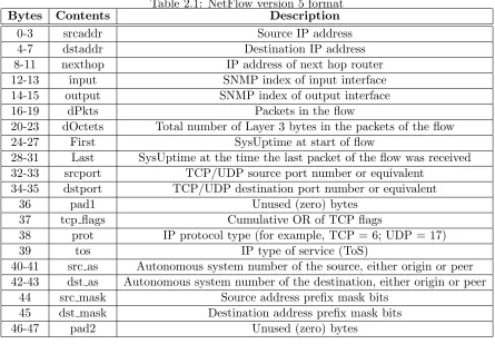
Table 2.1: NetFlow version 5 format
Bytes Contents Description
0-3 srcaddr Source IP address
4-7 dstaddr Destination IP address
8-11 nexthop IP address of next hop router
12-13 input SNMP index of input interface
14-15 output SNMP index of output interface
16-19 dPkts Packets in the flow
20-23 dOctets Total number of Layer 3 bytes in the packets of the flow
24-27 First SysUptime at start of flow
28-31 Last SysUptime at the time the last packet of the flow was received 32-33 srcport TCP/UDP source port number or equivalent
34-35 dstport TCP/UDP destination port number or equivalent
36 pad1 Unused (zero) bytes
37 tcp flags Cumulative OR of TCP flags
38 prot IP protocol type (for example, TCP = 6; UDP = 17)
39 tos IP type of service (ToS)
40-41 src as Autonomous system number of the source, either origin or peer 42-43 dst as Autonomous system number of the destination, either origin or peer
44 src mask Source address prefix mask bits 45 dst mask Destination address prefix mask bits
46-47 pad2 Unused (zero) bytes
• NetFlow Data Ware Housing and Data Mining NetFlow data can be hub for retrieval and analysis in support of applications according to user behavior. In addition, the Market Researchers access gain crucial information of ”who”, ”what”, ”where” and ”how long”
information relevant to the service providers.
Table-2.1 is reproduced from [3] for illustration of NetFlow Version 5 packet format. NetFlow
flows records are forwarded to the collector in form of UDP/IP packets. It can be heavy in computation for high speed network enivornment [3]. NetFlow features provide considerable
revelance for IP traffic under test. From symmetic uncertainity of all features, source and
destination IPs, source and destination ports, and TCP flags show high relevance. The reason is that IP address consist of social behavior of various applications such as HTTP servers, Mail
servers [24]. Hence, in our analysis, we consider high relevance flow attributes - source IP,
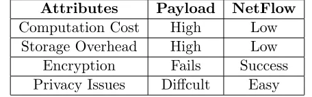
Table 2.2: Comparison between payload and NetFlow Attributes Payload NetFlow Computation Cost High Low
Storage Overhead High Low Encryption Fails Success Privacy Issues Diffcult Easy
Packet vs NetFlow
We provide an evaluation of advantages and disadvantages of payload and NetFlow methods as follows:
Processing at network speed for payload methods is high due to system memory bus
bot-tlenecks. With increase in volume of packets, there is risk to packet loss at high utilizations of a monitored link. In NetFlow, header information of all packets communicated between two
hosts accurately depicts IP traffic characteristics.
Storage requirements increases significantly for payload methods if packet size increases. On the other hand, flow sampling could reduce storage overhead.
Encryption causes signature matching in payload methods to fail. Alternatively, header
information remains unencrypted hence flow statistics can be computed.
Privacy Issues, due to RIAA litigations, has made providers reluctant to allow payload
analysis. Flow methodology provides an better solution to many privacy and legal issues rised
due to deep packet inspection.
2.2
Related Work
A number of techniques are used for accurate network application classification using port infor-mation, transport layer attributes, machine learning alogrithms or statistical models.
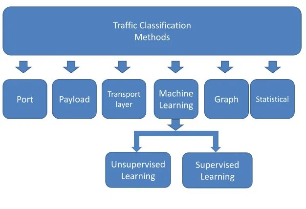
Figure-2.1 has shown the hierarchy of the various classification methods. We will briefly explain each
technique in the following sections.
2.2.1 Port-based Classification
IANA assigns port numbers for Internet applications for performing their operations. Port
based classification inspects the port numbers of the traffic to classify applications. Many applications deviate from standard port numbers to avoid detection and bypass firewall. Due
to rise of peer-to-peer applications, dynamic port allocation does provide accurate classification
Traffic Classification Methods
Port Payload Transport layer Machine
Learning Graph Statistical
Unsupervised Learning
Supervised Learning
Figure 2.1: Various Network Traffic Classification Methods
For byte based accuracy, the accuray was observed to be no better than 70% . For flow
accuracy, the value of accuracy fell to 30-50% . Hence, port numbers has been less reliable due
to deviatation from conventional port numbers [14].
2.2.2 Payload-based Classification
Payload-based classification identifies charateristics bit strings in packet payload that depict
controlling signals for a particular application. This method are applied majorly for peer-to-peer application and intrusion detection traffic due to their variant nature. Signatures are
derived from frequent bit patterns, string position, fixed or variable offset and even behavioral
signatures [15].
For peer-to-peer applications-, the overall accuracy is as high as 97.39%. Moreover,
combi-nation of port and payload based classification increases accuracy to almost 79% [18]. Although
payload classification provide more reliable and accurate results than port based classification, it imposes processing and storage overhead constraints. The generation of application
signa-tures is a tedious process with intense string searching and pattern matching. Signasigna-tures needs
to updated frequently as new trends in the applications are evolved. Hence, payload classifica-tion does provide considerable accuracy but at the cost of processing, storage and computaclassifica-tion
2.2.3 Transport-layer based classification
Port-based had limitations of reliability and low accuracy whereas payload-based had large
processing and storage requirements. To overcome these limitations, transport-layer heuristics
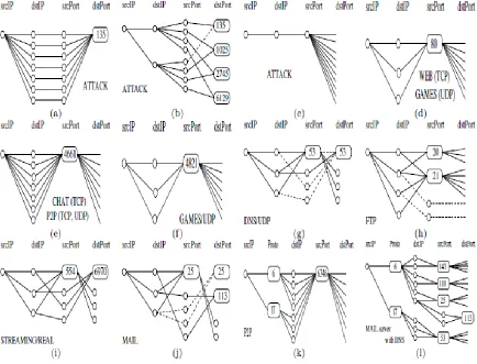
identifies unique behavior patterns of applications during transferring and signalling phase. They utilize only transport layer header information for flow traffic. From Figure-2.2 reproduced
from [12], we can see the interaction between hosts at various social, functional and application
level defines heuristics for classification.
Figure 2.2: Application behavior patterns based on transport layer attributes
From [12], we can observe that there are more that 90% flows with high accuracy values of
95%. Futhermore, both accuracy and completeness exceeds 80%. It overcomes limitations of
not distinct applications such as eMule, BitTorrent. In addition, the behavior of hosts are more
prominent at the edge of the network and hence limiting its use in the backbone networks.
2.2.4 Machine Learning
Machine learning (ML) techniques has two phases- training and testing. In the training phase,
the heuristics is built for the classification model. The training dataset analyzes characterisitics
of flow datasets to build the classification model. The model is then subjected to test dataset for classification of applications.
Figure 2.3: Application behavior patterns based on transport layer attributes
Figure-2.3, reproduced from [16], provides us understanding of network traffic classification by ML-based model. The ML-based classification model working can be illustrated as follows
[16]:
1. Real Time Traffic Capture−Network traffic is mirrored to a particular port and then collected in a memory unit. The collection can take place at backbone of the network
some classification methods. For instance, classification based on transport layer attribute
determinng host behaviors become more effective at the edge of the network.
2. Flow Statistics Processing − The captured packets are converted to flows. Various statistics related to flows such as mean packet inter-arrival time, medialn packet length
or flow duration are calculated. NetFlow becomes a convenient tool for capturing and processing network traffic in such class model.
3. Data Sampling−There are large data sets captured for a particular session of captured traffic trace. Processing and memory power required for these operation is extremely high. Data sampling provides us means to narrow down searches in large datasets without losing
valuable information.
4. Training Process−A fraction of dataset is used for training the classification algorithm. The training datasets helps to understand characteristics of flow traffic and enhances
classification for testing dataset. Training data set continously updates the model in real
time to keep itself updated with changing behavior patterns.
5. Classification Model−Classification model consist of various clustering, data mining, and information heuristics techniques. Classification learning involes machine learning
from training phase to build a set of classification rules to classify unseen traffic. During training, behavior patterns are analyzed in various application classes. During testing,
the traffic flow matching such patterns and charateristics are classified accordingly.
6. Classified Output − Flows are labeled with application class according to the classi-fication model. There can be clustering of flow sets with similar characteristics. Any
association between feature can also be presented with a probabilistic estimatation.
There are two types of ML techniques − Supervised learning and Unsupervised learning. Supervised learning requires learning phase to map the ML classes to application. For this reason, this ML is more popular for application identification for a particular group of class.
Unsupervised learning relies on automatic discovery of classes through clustering of datasets.
The clusters needs to be labeled to a particular application through direct inspection by a human expert [16].
There are number of algorithms such as EM algorithms, Naive Bayes, k-NN used for machine
learning technique of network traffic classification. We observe high accuracy of 81.51 % for unsupervised classifier using Naive Bayes. Moreover, there was higher accuracy of 90.51%
achieved for AutoClass unsupervised learning technique. Due to use of flow statistics, storage
recognized due to unsupervised clustering techniques. But there is need of human intervention
for accurately mapping groups clusters to application class [6].
2.2.5 Graph
In [10], network traffic is analyzed in an innovative by looking at flows in form of Traffic
Disper-sion Graphs (TDG). The graph based peer-to-peer detection (Graphtion) causes partitioning
traffic flows into clusters depending on flow attributes. Figure-2.4, reproduced from [10], shows the graph-based interaction of various hosts for client-server for HTTP application.
Figure 2.4: Graph-based classification for HTTP-TG application
In this method, there is around 90% precision and recall for peer-to-peer detection. For a
of the method is that there is estimation of number of clusters required forK-Mean algorithm.
2.2.6 Statistical Classification
The basis of this method is that applications has unique statistical characteristics such as bytes, duration, packet interarrival times, flow duration. These attributes help distinguish different
applications by finding relationship between traffic class and its observed statistical properties
[16]. As noted in [19], the connection characteristics are analysed for constructing empherical models using bytes, duration, arrival periodicity for a number of TCP connection.
The statistical methods observe accuracy values of 80-90% for internet chat systems [4]. But there are limitation due to its dependency on link utilization and network performance. Critical
attributes as distribution of interarrival times are heavily dependent on link utilization and
Chapter 3
Classification Model
In this chapter, we are going to understand the classification model for achieving accurate flow classification by using clustering and associative rule mining techniques. The main motive is
to combine unsupervised learning techniques with associative rule mining to achieve finer and
more accurate flow classification model.
3.1
Classification Model
The main part of the algorithm consists of unsupervised learning techniques with associative
rule mining, to achieve finer accurate flow classification. The methodology that was followed
is depicted in Fig.3.1 and was determined such that its implementation is similar to the one developed in [16].
3.1.1 Processing and Flow Data Processing
Libtrace is used to process trace file in legacy ATM format to pcap format [5]. In order to
convert the pcap traces to flows, we used conversation option of tshark tool [23]. The output
flows are conversation between two hosts with IP, port, duration and packet size information. The flow output from tshark is parsed and stored in the database. The following parameters
attributes of the flow are stored in the database.
1. Source IP
2. Source Port
3. Destination IP
Processing & Flow Data
Transductive Classification
Clustering Association
Rule Classification
Classified Output Machine Learning
Classification Process
Figure 3.1: Classification Model
Table 3.1: Distribution of application class in traces
Application Class No. of Flows Flow Proportion Port Number
HTTP 24568 9.3% 80, 443
DNS 9284 3.5% 53
SMTP 2197 0.83% 25
MAIL 1464 0.55% 110
IRC 553 0.21% 113
5. Source Byte and Source Packets
6. Destination Byte and Destination Packets
7. Total Byte and Total Packets
8. Protocol
Trace Statistics and Methodology
Port-based classification is used for defining application class of a particular flow. Since the
traces are captured for year 2001, peer-to-peer applications were not prevalent leading to well
behaved network traffic with standard port numbers. We summarize traffic class distribution in our traces as follows.
As the classes are not evenly distributed, the training sets will not present accurate results
data set for the classification model. This allows a fair training for the classification model with
no redundancy and equal application class distribution.
3.1.2 Clustering
We implement unsupervised learning techniques for classification. Due to ever changing
appli-cation patterns, we choice clustering technique to discover natural clusters in the data using
internalized heuristics. They define cluster flows with similar patterns or properties according to evaluation metrics such as Euclidean distance, entropy or Bayesian information number.
There are two clustering methods evaluated in this work - K-Mean and Model-based clustering methods.
K-Mean Clustering
K-Mean Cluster method uses attributes of datasets to cluster objects in to k-partitions. The
sum of squared distances from each data point to cluster center is minimized iteratively. The
squared error function is given as,
E=
k
X
i=1
X
xj∈Si
|xj−µi |2
where there are kclustersSi, i = 1,2,...,k and µi is mean value of all the pointsxj ∈Si.
The algorithm randomly partitions dataset into k-clusters. For each k clusters, the mean
values is calculated. The intra-cluster variance or squared error function is calculated for each data with respect to all mean values. The clusters are recomputed in a way to reduce square
error value iteratively. The algorithm converges when data point no longer switch clusters.
In our work, R function kmean is used for k-means analysis. There are two arguments of the functions - number of clusters (k) and number of iteration (iter.max). After number of
iteration, we were able to empirically conclude the value of iteration to be 10. The value of k
was increased to understand the growth in accuracy, precision and recall of each application class.
K-Mean method is extremely fast and with quick convergence. But there is need to estimate
number of clusters (k). The algorithm is more effective for spherical clusters naturally present in the dataset. Also, due to random selection of clusters, the results will not be same for each
Model-based Clustering
Model-based clustering is used for grouping flow data and based on a strong framework to
derive knowledge from data. This clustering technique is built on an assumption that data were
generated by a particular model and tries to find the original model from data. With number data model recovered, the number of clusters and its characteristics can retrieved. In general
model-based clustering, the model parameter is selected by maximum likelihood criterion that
maximizes the log-likelihood of generating data. Model-based clustering is more flexible. The adaptive nature is advantageous for various distributions of data such as Bernoulli, Gaussian
with non-spherical variance, or member of different family [7].
In MCLUST package, Bayesian Information Criterion (BIC) provide comprehensive strate-gies for parameterization and estimation of number of clusters. Maximum Likelihood is used as
a criterion for estimating the model. The prediction of number of clusters is achieved by using Bayesian Information Criterion.
A normal or Gaussian mixture model is assumed,
n Y i=1 G X k=1
τkφk(xi|µk,Σk)
where,
x = data
G = number of components
φk(x|µk,Σk) = (2π)
−π
2 exp{−1
2(xi−µk)TΣ
−
k1(xi−µk)}
τk = probability that an observation belongs to the kth component(τk≥0;sumGk=1τk= 1) n = number of data points
Σ = covariance matrix
The classification likelihood with parameterized normal distribution assumed for each class:
n
Y
i=1
φli(xi|µli,Σli)
where li= labels indication a unique classification of each observation;li=k ifxi belongs
to thekth component.
Ellipsoidal distribution centered at means µk is observed for both component and cluster models. Geometric features are determined by covariances Σk. Each covariance matrix is
paratermized by eigen value decomposition in the form
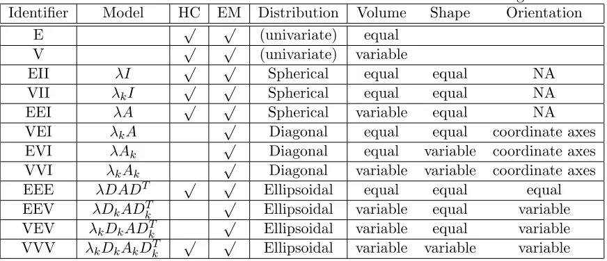
Table 3.2: Parameterization of Covariance Matrix in Mclust Package
Identifier Model HC EM Distribution Volume Shape Orientation
E √ √ (univariate) equal
V √ √ (univariate) variable
EII λI √ √ Spherical equal equal NA
VII λkI
√ √
Spherical equal equal NA
EEI λA √ √ Spherical variable equal NA
VEI λkA
√
Diagonal equal equal coordinate axes
EVI λAk
√
Diagonal equal variable coordinate axes VVI λkAk
√
Diagonal variable variable coordinate axes
EEE λDADT √ √ Ellipsoidal equal equal equal
EEV λDkADTk √ Ellipsoidal variable equal variable
VEV λkDkADTk √ Ellipsoidal variable equal variable
VVV λkDkAkDTk
√ √
Ellipsoidal variable variable variable
where,
Dk = orthogonal matrix of eigenvectors
Ak = diagonal matrix whose elements are proportional to the eigenvalues of Σk λk = scalar
In the model, principal component orientation for Σk depends on Dk. Also, the shape of
the density contours is determined byAk. Volume of the corresponding ellipsoid is specified by λkm which is proportional to λdk |Ak| where d represents data dimension. The characteristics
of the geometric features −orientation, volume and shape are estimated from data. These can vary between clusters, or restricted to the same for all clusters. In one dimension dataset, equal
variance and varying variance is represented by E and V respectively. For multiple dimensions, geometric characteristics of the model such as volume, shape and orientation is taken into
consideration. We can see from Table-3.2 that there are 9 models available in the Mclust.
The volume, shape and orientation represents clustering of flow data. In our case, VEV model represents volumes of all clusters as varying (V), shapes of all clusters as equal (E) and
orientation of all clusters as varying (V). BIC is an approximation to the Bayes factor. It adds
a penalty term on the log-likelihood depending on number of parameters.
BIC(k,Σ)≡2∗p(x|Θ, k,Σ)−v(k,Σ)∗log(n)
where, k is the number of clusters, p is the conditional probability; π stands for different variance-covariance structures andv(k,Σ) is the number of free parameters in a model with k
and model with the highest BIC is the best model for the flow dataset.
3.1.3 Transductive Classification
Due to clustering, we have grouped data sets with similar properties. These clusters need to
map to application class using a function or algorithm. Transductive classifier can be applied
to any clustering technique for classification. Consider train set is represented by Xm. There are l number of classes already labeled for the train set where i = 1,2,3, .. ,l. Now, Xn is test set in the model. We feed complete train and test set Xm+n to clustering method. The clustering methods partitions in to k-subsets. To find the class of a particular cluster, we need to find most common labels in that cluster according to train set labels. After clustering, the
transductive classifier algorithm can be built as follows,
• Label cluster with class iif the most common label in the cluster is i,i∈ 1, 2, .. l.
• Select uniformly at random any value of i for tie between two or more labels in a cluster or when no labels present.
The transductive classifier searches for labels from training datasets in the cluster. It labels application class corresponding to the most common label in the cluster. The remaining data
points have high probability of having similar properties as they are clustered together
depend-ing on algorithm heuristics. Thus, transductive classifier maps application class to clusters depending on train dataset labels.
3.1.4 Association-Rule Classification
Association Rule Classification unit provides a second level of heuristics to achieve finer clas-sification. Association rules find regularities between flow parameters with different measures
of interestingness for applications from transductive classifier output. Apriori Algorithm is
used for association rule learning [1]. The derived rules are traced back in the main trace and identified flows attain high accuracy, as will be shown in the next section. Moreover, the rule
association also helps predict IPs and ports used for servicing an application in the future. The
rules heuristics applied to flow data causes accurate classification and thus making classification method finer due to association rule mining techniques.
The association rule mining technique help we derive valuable relations within the data
points. In our case, such association will help us recognize pattern in a particular application. The goal of the data mining and classification models is to build a heuristic for predictive
recognizing the occurrence of application class from the data points.
an-tecedent. In other words, an event occurring due to antecedent is followed by the consequent
is depicted by the association rules for a particular class. The rules are represented as,
Antecedent => Consequent
Each rule is associated with three parameters, [1].
1. Support is the percentage of transactions that the rule can be applied to (the percentage
of transactions, in which it is correct).
2. Confidence is the number of cases in which the rule is correct relative to the number of cases in which it is applicable (and thus is equivalent to an estimate of the conditional
probability of the consequent of the rule given its antecedent).
3. Lift is the ratio of the probability that antecedent and consequent occur together, to the
multiple of the two individual probabilities for antecedent and consequent. There are
conditions where both support and confidence is high, and still result in to invalid rule. Therefore Lift indicates the strength of a rule over random occurrence of antecedent and
consequent, given their individual support. It provides information about improvement and increase in probability of consequent for a given antecedent. In the other words, Lift
is given as,
Rules with lower lift and confidence values are filtered out. Confidence is measured for
certainty of the rule. It measures event’s item set that matches antecedent of the implication
in the association rule and also matches consequent. The association rule indicates an affinity between antecedent and consequent with evaluation parameters such as Support, Confidence
and Lift.
Apriori Algorithm
Apriori Algorithm are based on the concept ofprefix tree. There are two steps for this algorithm
− frequent item sets and rule generation. In frequent item sets, the set of items maintaining least support are filtered. In the second phase, there will be rule generation from the computed
frequent item set. Apriori gains high efficiency by observing no superset of an infrequent item set.
Algorithm 1 has Apriori property stating that any subset of frequent item set must be
frequent. Join operation has a set of candidate k-item sets by joining Lk+1 with itself to find
Lk. Lastly, frequent item set are sets of item with minimum support. This represented by Li
Algorithm 1 Apriori Algorithm
Ck: Candidate item set of size k Lk: frequent item set of sizek Lk ={frequent item s}
for k= 1; Lk=φ;k++ do
Ck+1 = candidates generated fromLk
fortransaction tin database do
Increment count of all candidates in Ck+1 that are contained in t
Lk+1 = candidates inCk+1 with minimum support
end forreturn ∪k Lk
Chapter 4
Analysis and Results
In this chapter, we evaluate our classification model for two clustering methods -K-Mean and Model-based clustering with second level of classification heuristics using Apriori algorithm.
We perform cluster analysis and application profiling for understanding behavior patterns with
probabilistic prediction for each classified flow.
4.1
Traces
Waikato Internet Traffic Storage (WITS) is an open community for collecting data traces for
traffic measurement and identification research. Auckland VI traces for 2001-06-11 are used for analysis and testing of classification model. TCP, UDP and ICMP traffic and packets are
zeroed for length more 64 bytes. Anonymised IP are having one to one mapping for IP in the
range 10.0.0.0/8. The direction of the traffic coming towards the University Network [2]. Community Resource for Archiving Wireless Data At Dartmouth (CRAWDAD) provide us
with wireless traces for research community. Packet headers from every wireless packet sniffed in four of the campus buildings. The buildings were among the most popular wireless locations
in 2001, and included libraries, dormitories, academic departments and social areas. The MAC
address were sanitized by randomizing bottom six hex digits. IP address are anomalized using prefix-preserving IP sanitizer as described in [25]. In this technique, the two IP addresses
sharing the same k-bit prefix result in to a sanitized address with same k-bit prefix [13].
4.2
Classification Metrics
The classification model is evaluated by the conventional machine learning metrics such as
Precision, Recall and Accuracy [6]. The data set from classification algorithms can be placed
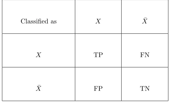
Table 4.1: Evaluation Metrics for Machine Learning Classification Techniques
Classified as X X¯
X TP FN
¯
X FP TN
used as evaluation parameters for machine learning classification algorithms.
Table-4.1 explains relationship of True Positive, False Positive, False Negative and True
Negative. In rows, X is represented as positive presence and ¯X is represented as negative presence. In columns, X is represented as True value and ¯X is represented as False value.
1. True Positive(TP): Total percentage of members (in our case flows) classified as Class A
belong to Class A.
2. False Positive(FP): Total percentage of members of Class A but does not belong to Class A.
3. False Negative(FN): Total percentage of members of Class A incorrectly classified as not belonging to Class A.
4. True Negative(TN): Total percentage of members which do not belong to Class A are
classified not a part of Class A. It can also be given as (100% - FP).
These metrics will help us form the overall accuracy, precision and recall of the classification model. We define these terms as follows:
Precision is given as the ratio of True Positives to True and False Positives. This value helps us understand the classification capability to identify objects correctly.
P recision= T rueP ositive
Recallis given as the ratio of True Positives to True and False Negatives. This value helps us understand the classification capability to determine misclassified members are something else.
Recall= T rueP ositive
T rueP ositive+F alseN egative
Overall Accuracyis given as the ratio of all True Positives to all True and False Positives for all classes.
OverallAccuracy =
Pn
i=1(T rueP ositive)
Pn
i=1(T rueP ositive+F alseP ositive)
4.3
Analysis and Results
We have utilized two clustering algorithms- Kmean and Model-based clustering algorithms. For
Kmean clustering, k indicates the number of clusters and varied from 50 to 500 with a step
of 50. For Model-based classification, there is no need estimation of number of clusters in the dataset. Each algorithm clusters are passed through transductive classifier and finally precision,
recall and accuracy is calculated and plotted. The following section will have analysis of each
algorithm with their respective performance graphs.
4.3.1 K-Mean Clustering Precision Graph
The values of precision increases considerably as number of cluster increases as seen
fromFig-ure 4.1. Value of precision is in the vicinity of 60% for all applications for K<100. We observe that the value of precision reaches a high value but with a tradeoff of large number of clusters. For k = 500, the precision is in the vicinity of 92% but test data set is 1000 flows.
As the number of cluster size increases, the number of flows in each clusters become smaller.
For every iteration, the mean value for each cluster is tightly bound with other flows in the cluster as it eliminates false positive flows in each cluster.
Large cluster number will cause heavy computation stress on the classification as each cluster will assist in deriving application patterns. As precision is a measure of classifier ability to find
correct flows in a class, we would interpret that it performs fairly for increase in k.
Recall Graph
Recall gives us the measure of the rejection of flows from the other class. The flows from other
`
50 60 70 100 150 200 250 300 350 400 450 500
0 10 20 30 40 50 60 70 80 90 100 KMean Transductive Classifier Precision Graph
http mail smtp dns irc
Cluster Size (k) P re ci si on ( % )
Figure 4.1: K-Mean Transductive Classifier Precision Graph for WAND Traces
`
50 60 70 100 150 200 250 300 350 400 450 500
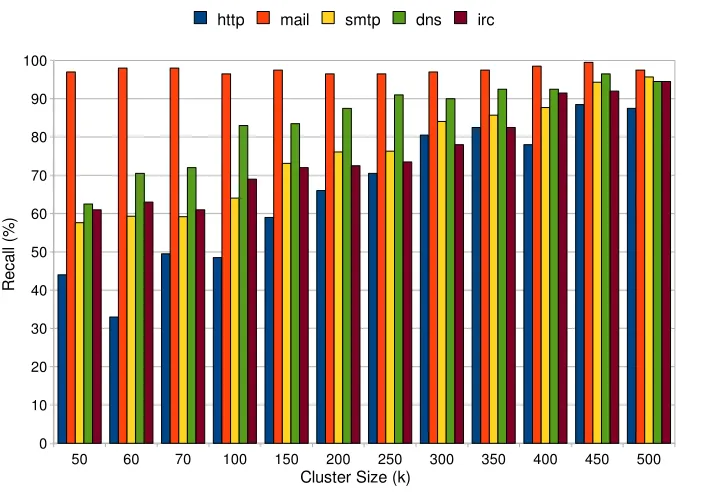
0 10 20 30 40 50 60 70 80 90 100 KMean Transductive Classifier Recall Graph
http mail smtp dns irc
Cluster Size (k) R ec al l ( % )
for high values of k. We have observed recall in the vicinity of 94% for k>400 for all application class.
Accuracy Graph
`
50 60 70 100 150 200 250 300 350 400 450 500
0 10 20 30 40 50 60 70 80 90 100 KMean Transductive Classifier Accuracy Graph Cluster Size (k) A cc ur ac y (% )
Figure 4.3: K-Mean Transductive Classifier Accuracy Graph for WAND Traces
From Figure 4.3, the overall accuracy is given by the aggregate of precision for all the
application class. We observe high accuracy of 92% for k= 500 and low accuracy of 64% for k=50. As the have been growth of precision for all the classes, this has been well reflected with
high overall accuracy.
The growth in the precision and recall of the cluster is due to fine segmentation of the flow clusters due to increase in cluster number. As there is increase in number of clusters, the
K-Mean iteration for each k cluster are more tightly clustered by reducing within-cluster sum of squares. This results in to clusters of particular application class with unwanted flows from other class being eliminated. We can see very evidently with increase in precision for all the
application class.
application class observe different behavior, the value of k cannot simply be equal to number of
application class. Hence it is difficult to estimate k value for each new dataset as well as maintain high accuracy and precision. Moreover, large flow sets will have limitation of processing power
due to high iteration required for accurate results.
4.3.2 Model-based Clustering
Figure 4.4: Bayesian Information Criterion distribution for parameterization
Mclust uses Bayesian Information Criterion to estimate models and number of clusters.
From Fig.4.4, we can see that BIC value for each of the nine models is calculated. The model with the highest value will be chosen as the best estimate of the input data. In our case,
BIC is strongest for number of components equal to 9 corresponding to VEV model. VEV
model represents volumes of all clusters as varying (V), shapes of all clusters as equal (E) and orientation of all clusters as varying (V). BIC is an approximation to the Bayes factor. It adds
a penalty term on the log-likelihood depending on number of parameters. The best model
estimated is VEV model. VEV indicates volume and orientation is variable (V) and shape is equal (E) resulting intoEllipsoidal distribution. The number of clusters is very close to number
Flow sets have source and destination IP and port numbers and hence can be described as
multidimensional dataset. Hence , we can observe that geometric features come in to consid-eration for data model. From the model, we can estimate that flow points will be ellipsoidally
placed in space.
Precision Graph
`
http mail smtp dns irc
0 10 20 30 40 50 60 70 80 90 100 Modelbased Transductive Classifier Precision Graph Application P re ci si on ( % )
Figure 4.5: Model-based Transductive Classifier Precision Graph for WAND Traces
By narrowing down a particular data model for test data, Mclust accurately estimates the
clustering parameters using BIC . VEV indicates volume and orientation is variable(V) and
shape is equal(E) with Ellipsoidal distribution.
Model-based hierarchical clustering is used for this particular ellipsoidal distributed data
model. Each flow behaves as an individual cluster and pairs are merged as it progresses up
the hierarchy. This is bottom-top approach as individual flows are considered as initialization point. Thus, flows with similar properties are clustered together as it moves up the hierarchy.
strong precision for 100% for HTTP, IRC and SMTP flows.
Recall Graph
`
http mail smtp dns irc
0 10 20 30 40 50 60 70 80 90 100
Modelbased Transductive Classifier Recall Graph
Application
R
ec
al
l (
%
)
Figure 4.6: Model-based Transductive Classifier Recall Graph for WAND Traces
False positive rejection has been prominent for SMTP application. SMTP applications are used for mail relaying, user-client application and delivery only protocol. Hence, SMTP flows
are communicating with mail server on set of port numbers resulting into strong clustering.
This can be reinforced due to high precision value for SMTP. The recall is consistent for HTTP, DNS, IRC, Mail The rejection is strong of order of 80% for most the applications.
Overall Accuracy
Cluster Size Overall Accuracy
9.0 81.5
The overall accuracy is higher for this particular clustering classifier. As the number of
Table 4.2: Precision & Recall for TranductiveK-Mean and Model-based classification Application K-Mean Precision Model Precision K-Mean Recall Model Recall
http 79.58 100 65.63 81.5
mail 86.68 73.02 97.5 78.5
smtp 76.1 100 76.1 100
dns 76.12 55.28 84.67 78.5
irc 75.42 100 75.88 69
The package has features of combining model-based hierarchical clustering, expectation
and maximization for Gaussian mixture models with parameter estimation using BIC. The
probability density function is calculated for observation belonging to each class. A covariance matrix (i,j) is derived with probabilistic value of ith flow belonging to the jth class. Hence, due
to the data modeling and parameter estimation, the clustering algorithm converge to a finer
flow classification [7]. Moreover, the number of cluster is predicted by BIC and is also very close to the actual number of application class.
The gain in accuracy is because model-based clustering techniques assumes data belongs to a particular model. There is an accurate estimation of model leading enhanced clustering. As
opposed toK-Mean, there is no need of human intervention for predicting cluster size for each flow data.
4.3.3 Rule based Classification
Fig.4.7 shows accuracy for K-Mean clustering followed by Apriori Algorithm. There are weak association inK-Mean clusters because there is fall in accuracy for all application class.
SMTP observed lower accuracy for all the range of cluster size. SMTP have user-client application and messaging services running for a particular host. The messaging services varies
in destination port numbers. Moreover, relaying of services for mail services results in varied
host IPs. K-Mean clustering does not accurately converge to the mean values for this application class. One of the reason is that mean values are randomly selected for initialization of the
algorithm.
On the other hand, HTTP and DNS have gained high accuracy due to client-server protocol behavior. HTTP servers and DNS servers are set of host application that are constantly being
communicated by user hosts. These IP are clustered together due to few servers to many client communication patterns.
The goal of the second level of association rule classification is to identify flows and segregate
0 250 300 350 400 450 500 10
20 30 40 50 60 70 80 90 100
KMean and Rulebased Classification Accuracy Graph
http mail smtp dns irc
Cluster Size
A
cc
ur
ac
y
(%
)
Figure 4.7: K-Mean and Rule-based Classification Accuracy Graph for WAND Traces
clusters map to flows with other application class indicating poor false positive rejection.
Fig.4.8 refers to model-based clustering with apriori algorithm for association rule
classifi-cation. Due to accurate model estimation capability, the nature of the cluster is predicted with Bayesian Information Criterion. The estimation leads to appropriate choice of distribution,
leading to an enhanced clustering result.
Association rule based on flow attributes identify accurately flows having similar application behavior. Due to strong data evaluation capability of Model-based clustering, the association
rule heuristics have high confidence value for application class.
We tested our classification model with other traces to nullify dependency of particular network or data traces. Crawdad data traces does observe accuracy on similar range as WAND
traces. WAND traces average accuracy comes up to 94% and Crawdad comes around 93%. As
`
http mail snmp dns irc
0 10 20 30 40 50 60 70 80 90 100
Modelbased and Rulebased Classification Accuracy Graph
WAND Crawdad
Application
A
cc
ura
cy
(%
)
Figure 4.8: Model-based clustering and Rule based classification Accuracy for WAND and Crawdad traces
Table 4.3: Accuracy for Association Rule classifier based onK-Mean and Model-based cluster-ing for WAND and CRAWDAD Traces
Application K-Mean Accuracy WAND Trace CRAWDAD Trace
http 61.48 100 100
mail 42.94 94.05 87.82
smtp 11.28 89.34 94.87
dns 61.67 92.11 88.15
Figure 4.9: Distribution of flow attributes in scatter plot matrix
4.4
Cluster Analysis
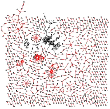
In Fig.4.9, the distribution of IP and ports for source and destination is depicted for
Model-based clustering method. The graph has diagonal blocks mentioned with the parameters in
that row and column. In order to consider source and destination IP distribution, we need to go at plot interesting source IP row/column and destination IP row/column.
• For HTTP (blue) application, large number of source IPs direct traffic too few destination IPs. HTTP behavior is prominent because a number of source hosts are communicating
with small number of destination hosts i.e. HTTP servers.
• In DNS application, source hosts communicate with a set of DNS servers. Each host interacts with different domains such as www, .org and .net for resolving IP addresses.
The DNS behavior is prominent because large group of source hosts communicate with
small repeated set of destination IPs.
• In IRC application, a group of hosts communicates with other group of hosts. There is roughly one-to-one correspondence between source and destination IP. This behavior is
prominent because IRC (cross) traffic has set of source IPs communicate with
• Moreover, source IP and destination port distribution show that destination port numbers are in the range of 30000 for SMTP (green) traffic. DNS destination ports are randomly distributed where as HTTP and MAIL have destination ports number in lower range of
1000.
4.5
Behavior Pattern for Application
The association rule mining technique help we derive valuable relations within the data points.
In our case, such association will help us recognize pattern in a particular application. The goal data mining and classification models is build a heuristics for predictive for recognizing
the occurrence of application class from the data points.
Rules with lower lift and confidence values are filtered out. Confidence is measured for certainty of the rule. It measures event’s item set that matches antecedent of the implication in
the association rule and also matches consequent. Table I clearly mentions flow parameters in
antecedent and consequent format for building association rules. The association rule indicates an affinity between antecedent and consequent with evaluation parameters such as Support,
Confidence and Lift.
For example, for HTTP, destination IP with index 1 and destination port number equal to 1273 will have a flow from source IP of index 233 with confidence (noted as C) of 1 and lift of 81.5. When we trace back this flow, we are accurately able to classify this flow as HTTP.
Moreover, in the future, if we observe any particular flow with this association then we would be certain to classify it as HTTP with confidence value of 1.
We can observe that each application are profiled according to their respective behavior.
Every rule confidence value tells us that flow with this particular association will be belonging to that corresponding application class. Thus, we understand the following for each application
behavior profiling: It is used for resolving host names with IP address. Domain Server services
queries for any particular host. Hence, we observe centralized architecture with client-server communication pattern. In Table-4.4, we can clearly observe that source and destination IPs
are associated with each other. There are host pairs (200,46), (187,32) and (19,69) representing
communication between host and domain server for DNS traffic. Various user messages are ser-viced by using mail application. There is a mail server servicing, routing and relaying messages
between two parties. The communication behavior of relaying and messaging is prominently
observed in Mail and SMTP application. In IRC application, different destination port number with set IPs communicating with each other is very well depicted.
Hence, we are able to gain higher accuracy by using apriori algorithm after transductive classifier. The design helps us find valuable association rules for classified data with estimation
Table 4.4: Association Rules from Apriori Association Algorithm
Traffic Rules Confidence Lift
DNS dip=16 =>dport=56322 1 21.8
dport=4207 => dip=43 1 17.7
dstip=19 =>srcip=69 0.02 35.5
srcip=69 =>dstip=19 0.02 35.5
srcip=200 => dstip=46 0.1 9.7
dstip=46 =>srcip=200 0.1 9.7
srcip=187 => dstip=32 0.2 3.5
dstip=32 =>srcip=187 0.2 3.5
Mail dip=8 =>dport=53 1 6.7
dip=16 =>dport=53 1 6.7
srcip=226 => dstip=49 1 53.75
dstip=49 =>srcip=226 1 53.75
dstip=8 =>dstport=53 1 6.7
srcip=200 => dstip=51 1 4.57
dstip=51 =>srcip=200 1 4.57
srcip=95 =>dstip=30 0.4 8.95
dstip=13 =>dstport=53 0.4 6.71
HTTP dip=1 & dport=1273 =>srcip=233 1 81.5
{} =>dip=1 0.7 1
srcip=139 => dstip=1 1 1.4
srcip=9 =>dstip=1 1 1.4
srcip=41 =>dstip=1 1 1.4
dstport=2006 =>dstip=1 1 1.4
dstip=41 =>srcip=164 40.75
srcip=233 & dstip=1 =>dstport=1273 1 81.5
IRC sip=162 =>dport=37273 1 69
{} =>dip=16 0.7 1
dstip=3 & dstport=39938 =>srcip=18 1 46 srcip=168 & dstport=37321 =>dstip=3 1 4.4 srcip=168 & dstip=3 =>dstport=37321 1 69 dstip=3 & dstport=37321 =>srcip=168 1 69 srcip=162 & dstport=37273 =>dstip=16 1 1.3 srcip=162 & dstip=16 =>dstport=37273 1 69 SMTP sip=262 & dport=4868 => dip=28 1 2.8
dip=28 & dport=4868 =>sip=262 1 15.3
srcip=196 => dstip=3 1 5.7
dstport=4706 =>srcip=261 1 22.2
dstport=4706 =>dstip=28 1 2.8
srcip=277 => dstip=43 1 7.1
srcip=241 => dstip=3 1 5.7
Chapter 5
Conclusion
5.1
Summary of Results
In this work, we have presented a classification model that achieves high flow classification accuracy with application behavior profiling. Association rules derived from transductive
clas-sification are fed back to refine clasclas-sification model. This leads to a finer clasclas-sification model
with much better accuracy. The rule heuristics are produced without any human intervention and become independent of dataset. In addition, our model is able to detect new behavior
patterns for next generation applications. We summarize our results in the following points:
• We built two level classification models with unsupervised learning techniques. Clustering transductive classification was used for first level and association rule mining for second
level of classification. Model-based clustering and Apriori Algorithm form basis of the
classification model.
• We achieve accuracy value of around 94%. The precision value for all application class remains high, and independent of trace sets.
• Each application has behavior profiling due to use of Apriori Algorithm. The behavior patterns tells us various flow attributes so that we can identify and classify flows in the
future.
• Each association rule is providing with confidence value to gain accurate results. More-over, support provides information of the number of flows present in the dataset. In addition, Lift defines strength of the relation between antecedent and consequent.
• Due to utilization of flow parameters, the processing and computational power is less. Large flow data sets can be analyzed with accurate results and application behavior
5.2
Future Work
In the future work, we are planning to capture trace files for reviewing our classification model.
We plan to analyze wide variety of applications with different behavior patterns and connection norms. With accurate classification, we want to build a prediction model for application class.
This will enhance the capability of classifying as well as monitoring of particular traffic in the
REFERENCES
[1] C. Borgelt and R. Kruse. Induction of association rules: Apriori implementation. In Comp-stat: Proceedings in Computational Statistics: 15th Symposium Held in Berlin, Germany, 2002, page 395. Physica Verlag, 2002.
[2] WAND Trace Catalogue. http://www.wand.net.nz/wits/catalogue.php.
[3] IOS Cisco. Netflow white papers, 2006.
[4] C. Dewes, A. Wichmann, and A. Feldmann. An analysis of Internet chat systems. In Proceedings of the 3rd ACM SIGCOMM conference on Internet measurement, pages 51– 64. ACM, 2003.
[5] Libtrace Documentation. http://www.wand.net.nz/trac/libtrace.
[6] J. Erman, A. Mahanti, and M. Arlitt. Internet traffic identification using machine learning. InProceedings of IEEE GlobeCom. Citeseer, 2006.
[7] C. Fraley and A.E. Raftery. MCLUST version 3 for R: Normal mixture modeling and model-based clustering. Technical report, Citeseer, 2006.
[8] P. Haffner, S. Sen, O. Spatscheck, and D. Wang. ACAS: automated construction of ap-plication signatures. In Proceedings of the 2005 ACM SIGCOMM workshop on Mining network data, page 202. ACM, 2005.
[9] IANA. Internet Assigned Numbers Authority (IANA).
http://www.iana.org/assignments/port-numbers.
[10] M. Iliofotou, H. Kim, M. Faloutsos, M. Mitzenmacher, P. Pappu, and G. Varghese. Graph-based P2P traffic classification at the internet backbone. InIEEE Global Internet Sympo-sium. Citeseer, 2009.
[11] T. Karagiannis, A. Broido, and M. Faloutsos. Transport layer identification of P2P traffic.
In Proceedings of the 4th ACM SIGCOMM conference on Internet measurement, pages
121–134. ACM, 2004.
[12] T. Karagiannis, K. Papagiannaki, and M. Faloutsos. BLINC: multilevel traffic classification in the dark. ACM SIGCOMM Computer Communication Review, 35(4):240, 2005.
[13] David Kotz, Tristan Henderson, Ilya Abyzov, and Jihwang Yeo. CRAW-DAD trace dartmouth/campus/tcpdump/fall01 (v. 2004-11-09). Downloaded from http://crawdad.cs.dartmouth.edu/dartmouth/campus/tcpdump/fall01, November 2004.
[15] A.W. Moore and K. Papagiannaki. Toward the accurate identification of network applica-tions. Passive and Active Network Measurement, pages 41–54, 2005.
[16] TTT Nguyen and G. A rmitage. A survey of techniques for internet traffic classification using machine learning. IEEE Communications Surveys & Tutorials, 10(4):56–76, 2008.
[17] I. Papapanagiotou and M. Devetsikiotis. Aggregation Design Methodologies for Triple Play Services. InIEEE CCNC 2010, Las Vegas, USA, pages 1–5, 2010.
[18] B.C. Park, Y.J. Won, M.S. Kim, and J.W. Hong. Towards automated application signa-ture generation for traffic identification. In IEEE Network Operations and Management Symposium, 2008. NOMS 2008, pages 160–167, 2008.
[19] V. Paxson. Empirically derived analytic models of wide-area TCP connections.IEEE/ACM Transactions on Networking (TON), 2(4):336, 1994.
[20] V. Paxson. Bro: A system for detecting network intruders in real-time.Comput. Networks, 31(23):2435–2463, 1999.
[21] M. Roughan, S. Sen, O. Spatscheck, and N. Duffield. Class-of-service mapping for QoS: a statistical signature-based approach to IP traffic classification. In Proceedings of the 4th ACM SIGCOMM conference on Internet measurement, pages 135–148. ACM, 2004.
[22] S. Sen, O. Spatscheck, and D. Wang. Accurate, scalable in-network identification of p2p traffic using application signatures. InProceedings of the 13th international conference on World Wide Web, page 521. ACM, 2004.
[23] tshark Documentation. http://www.wireshark.org/docs/man-pages/tshark.html.
[24] J. Wang, Z. Ge, H. Jiang, S. Jin, and A.W. Moore. Lightweight application classification for network management, July 2008.
Appendix A
Application Behavior Profiling
A.1
DNS behavior Pattern
no rules support confidence lift
1 srcip=180 => dstip=6 0.010 1 71
A.2
Mail behavior Pattern
No rules support confidence lift
A.3
HTTP behavior Pattern
No rules support confidence lift
1 {} =>dstip=1 0.711 0.711 1
2 srcip=139 =>dstip=1 0.012 1 1.40
3 srcip=9 =>dstip=1 0.012 1 1.405
4 srcip=41 =>dstip=1 0.012 1 1.405
5 dstport=2006 => dstip=1 0.012 1 1.405
6 dstip=41 =>srcip=164 0.01 1 40.75
7 dstip=55 =>srcip=164 0.012 1 40.75
8 srcip=11 =>dstip=1 0.012 1 1.405
9 dstip=53 =>srcip=242 0.012 1 81.5
10 srcip=242 =>dstip=53 0.012 1 81.5
11 srcip=6 =>dstip=1 0.012 1 1.405
12 srcip=134 =>dstip=2 0.01 1 54.3
13 srcip=439 =>dstip=1 0.012 1 1.405
14 srcip=407 =>dstip=1 0.0127 1 1.405
15 dstport=1273 =>srcip=233 0.012 1 81.5 16 srcip=233 => dstport=1273 0.012 1 81.5
17 dstport=1273 => dstip=1 0.012 1 1.405
18 srcip=424 =>dstip=1 0.012 1 1.405
19 srcip=233 =>dstip=1 0.012 1 1.405
20 srcip=409 =>dstip=1 0.0122 1 1.405
21 srcip=2 =>dstip=1 0.018 1 1.405
22 srcip=50 =>dstip=1 0.018 1 1.405
23 srcip=190 =>dstip=1 0.018 1 1.405
24 srcip=226 =>dstip=49 0.01 1 13.58
25 srcip=389 =>dstip=1 0.0181 1 1.405
26 srcip=382 =>dstip=1 0.011 1 1.405
27 srcip=408 =>dstip=1 0.024 1 1.405
28 srcip=338 =>dstip=1 0.024 1 1.405
29 srcip=75 =>dstip=45 0.024 1 32.6
30 dstip=45 =>srcip=75 0.024 0.8 32.6
31 srcip=344 =>dstip=1 0.024 1 1.405
32 srcip=444 =>dstip=1 0.030 1 1.405
33 srcip=155 =>dstip=1 0.024 0.8 1.124
A.4
IRC behavior Pattern
No rules support confidence lift
1 {} =>dstip=16 0.71 0.71 1
2 srcip=301 =>dstip=16 0.014 1 1.39
3 srcip=247 =>dstip=16 0.014 1 1.39
4 srcip=49 =>dstip=16 0.014 1 1.39
5 srcip=457 =>dstip=16 0.014 1 1.39
6 dstport=39938 => srcip=18 0.014 1 46
7 dstport=39938 =>dstip=3 0.0144 1 4.41
8 srcip=99 =>dstip=16 0.014 1 1.39
9 srcip=168 =>dstport=37321 0.014 1 69
10 dstport=37321 =>srcip=168 0.014 1 69
11 srcip=168 =>dstip=3 0.014 1 4.45
12 dstport=37321 =>dstip=3 0.014 1 4.45
13 srcip=162 =>dstport=37273 0.014 1 69
14 dstport=37273 =>srcip=162 0.014 1 69
15 srcip=162 =>dstip=16 0.014 1 1.39
16 dstport=37273 => dstip=16 0.01 1 1.39
17 srcip=292 =>dstip=3 0.014 1 4.45
18 srcip=428 =>dstip=16 0.014 1 1.39
19 srcip=316 =>dstip=16 0.014 1 1.39
20 srcip=209 =>dstip=16 0.014] 1 1.39
21 srcip=183 =>dstip=16 0.021 1 1.393
22 srcip=18 =>dstip=3 0.021 1 4.45
23 srcip=322 =>dstip=16 0.028 1 1.39
24 srcip=305 =>dstip=16 0.028 1 1.39