ABSTRACT
CHURCH, DAVID EARL. Long-lived African Easterly Waves. (Under the direction of Dr. Anantha R. Aiyyer.)
The first part of this study uses an observational approach to study long-lived African easterly waves (AEWs). Long-lived AEWs are defined to be waves that exit the coast of Africa and propagate to 60°W before either developing into a tropical cyclone (TC) or dissipating. These waves show resilience in crossing the tropical Atlantic without either developing into a TC or dissipating. The NHC Tropical Cyclone reports were used to identify long-lived, developing AEW cases, while the ERA-Interim reanalysis and TRMM 3B42 data sets were used to confirm and track these cases. In all, 29 long-lived, developing cases were identified within the 2000 to 2010 hurricane seasons, accounting for about 15% of all hurricanes during that period. Two case studies are examined and they reveal an association between convection within the wave and a strengthening wave, while a lack of convection was associated with a weakening wave. Expanding the analysis to all 29 cases also suggested that convection within the wave may be critical to maintaining the wave. Convectively active times in the 29 cases were linked to increasing wave-level potential vorticity (PV), while convectively inactive times were linked to decreasing wave-level PV. While the observational portion of the study suggests that convection is important to maintaining or strengthening the long-lived waves, it does not give information about the physical processes linking individual thunderstorm clusters and the generation of wave scale vorticity in the middle and lower troposphere.
Long-lived African Easterly Waves
by
David Earl Church
A thesis submitted to the Graduate Faculty of North Carolina State University
in partial fulfillment of the requirements for the Degree of
Master of Science
Marine, Earth & Atmospheric Sciences
Raleigh, North Carolina
2012
APPROVED BY:
Dr. Fredrick H.M. Semazzi Dr. Matthew D. Brown Parker
DEDICATION
BIOGRAPHY
I grew up in Virginia Beach, VA, where I spent my childhood fascinated by the weather in the region. I watched eagerly as thunderstorms built on hot summer afternoons, I would wait in suspense for the much anticipated snow storms in the winter (which disappointed more often than not), and I tracked the progress of the hurricanes in Atlantic and experienced the wrath of a few of those storms. I attended the Mathematics and Science Academy at Ocean Lakes High School, where I began building a solid foundation for my understanding and passion for science. With my strong background as a student, my passion for meteorology and encourage-ment from my family I attended North Carolina State University for my undergraduate degree in Meteorology. I graduated summa cum laude and among the top of my meteorology class in May 2009. I decided to continue on with my education in Meteorology by starting my work as a graduate student under the advisement of Dr. Anantha Aiyyer in August 2009.
ACKNOWLEDGEMENTS
TABLE OF CONTENTS
List of Tables . . . vii
List of Figures . . . .viii
Chapter 1 Introduction . . . 1
1.1 Introduction . . . 1
Chapter 2 Observational Study . . . 6
2.1 Data . . . 6
2.1.1 ERA-Interim . . . 6
2.1.2 TRMM 3B-42 . . . 6
2.2 Observational Wave Tracking and Identification . . . 7
2.2.1 African Easterly Wave Tracking Method . . . 7
2.2.2 Identification of Long-lived African Easterly Waves . . . 7
2.3 Climatology . . . 8
2.4 Observational Study . . . 9
2.4.1 PV Basics . . . 9
2.4.2 PV Flux into the Wave . . . 9
2.4.3 PV Generation from Convection: Case Studies . . . 10
2.4.4 PV Generation from Convection: Extension to all Long-lived Developing Cases . . . 12
2.4.5 Case Study: Ernesto 2006 . . . 13
2.4.6 Conclusions from the Observational Study . . . 15
Chapter 3 Modeling Study . . . 26
3.1 Modeling Study . . . 26
3.1.1 High Resolution Model Simulation . . . 26
3.1.2 Model Verification . . . 27
3.2 Modeling Results . . . 30
3.2.1 Wave Evolution and Wave Pouch Analysis . . . 30
3.2.2 Potential Vorticity Budget . . . 33
3.2.3 Potential Vorticity Budget Analysis . . . 36
3.2.4 Vorticity Budget . . . 40
3.2.5 Vorticity Budget Analysis . . . 41
3.3 Effects of Stratiform and Convective Precipitation . . . 45
3.3.1 Vorticity Budget for Convective vs Stratiform Regions . . . 46
3.3.2 Conclusions about Convective vs Stratiform Precipitation on the Wave . . 47
Chapter 4 Conclusions . . . 68
4.1 Conclusions . . . 68
4.1.1 Observational Study . . . 68
4.1.3 Final Thoughts . . . 72
LIST OF TABLES
LIST OF FIGURES
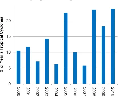
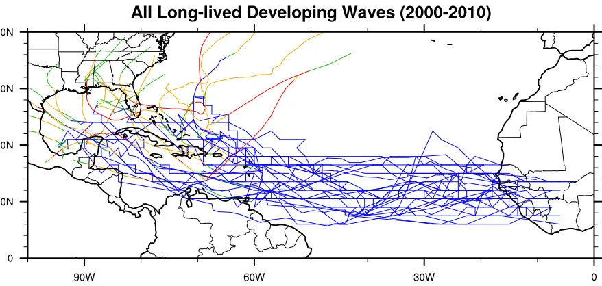
Figure 2.1 A histogram of the percentage of tropical cyclones that formed from long-lived AEWs each year between 2000 and 2010 . . . 17 Figure 2.2 Tracks of all 29 long-lived, developing AEW cases between 2000 and
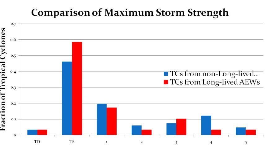
2010. Blue indicates a wave, green indicates a tropical depression, orange indicates a tropical storm and red indicates a hurricane. . . 18 Figure 2.3 Comparison of the maximum storm classifications for tropical cyclones
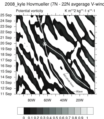
forming from long-lived AEWs (red) and those forming from non-lived disturbances (blue). . . 19 Figure 2.4 A Hovmoller diagram of 600 hPa PV from the pre-Kyle (2008) AEW
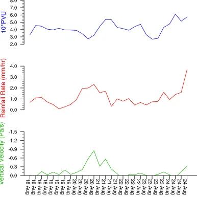
and its merger with a mid-latitude PV source prior to tropical cyclogen-esis. The ”*” symbol illustrates the point of merger and the ”X” symbol illustrates the point of TC genesis as denoted by the NHC. . . 20 Figure 2.5 A time series of the area-average (6°x 6°box) of the 600 hPa PV (top),
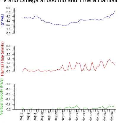
TRMM rainfall rate (middle) and 600 hPa omega (bottom) for the pre-Stan (2005) AEW. . . 21 Figure 2.6 A time series of the area-average (6°x 6°box) of the 600 hPa PV (top),
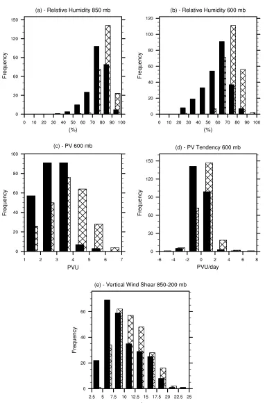
TRMM rainfall rate (middle) and 600 hPa omega (bottom) for the pre-Ernesto (2006) AEW. . . 22 Figure 2.7 Histograms that compare the non-convective (shaded) to the convective
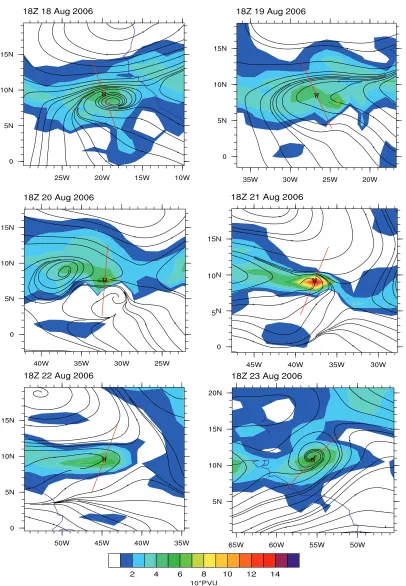
(hatched) reanalysis times for the 29 long-lived, developing AEW cases. . 23 Figure 2.8 600 hPa wave-relative streamlines and PV for the pre-Ernesto AEW
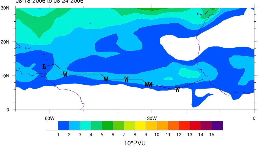
from the ERA-Interim reanalysis. . . 24 Figure 2.9 The wave track for the pre-Ernesto AEW overlaid on the time averaged
PV field from 18 August 2006 to 24 August 2006. . . 25
Figure 3.1 Model domains as initialized on 0000 UTC 18 September 2006. The outer domain is a 12 km fixed domain while the inner domain (d02) is a 4 km moving nest that remains centered on the pre-Ernesto wave. . . 48 Figure 3.2 Comparison between the WRF simulated AEW track (black line with
white dots and labels) and the ERA-Interim track (blue line) and NHC best track data (red line). . . 49 Figure 3.3 Comparison between the WRF simulations, ERA-Interim and NHC
Figure 3.4 Composite precipitation (mm/day) for the pre-Ernesto AEW. The WRF simulation (a) and the TRMM 3B42 (b) averaged between 0000 UTC 19 August 2006 and 0000 UTC 21 August 2006. (c),(d) as in (a),(b) except averaged between 0000 UTC 22 August 2006 and 0000 UTC 24 August 2006. (e),(f) as in (a),(b) except averaged between 0000 UTC 25 August 2006 and 0000 UTC 27 August 2006. . . 51 Figure 3.5 The result of a thought experiment to compare the typical Eulerian
view to the Lagrangian view of an AEW like vortex. Panel (a) shows a Rankine vortex embedded in easterly flow to represent a typical easterly wave. Panel (b) shows the same vortex with the same background flow, but subtracts a typical AEW phase speed from the total flow. The solid vertical lines indicate the wave trough, while the solid horizontal lines indicate the critical latitude for this case. The bold, solid contour in panel (b) indicates the boundary of the wave pouch, where the air inside this streamfunction line is recirculated and protected from outside intrusion. 52 Figure 3.6 Hovmoller plot of the 850 hPa v-wind averaged between 7°N and 17°N
for the pre-Ernesto AEW (2006) from the WRF simulation. The solid line denotes the trough axis. The three estimated phase speeds of the wave can be seen by the change in slope of the solid line with time. . . 53 Figure 3.7 PV and wave-relative streamlines in a 720 km x 720 km box, center on
the wave pouch. Plot levels increasing with height from bottom to top and time increasing from left to right. This figure illustrates the evolution of the wave pouch with height throughout the course of the simulation. . 54 Figure 3.8 Simulated radar reflectivity (DBZ) overlaid on 600 hPa wave-relative
streamlines in a 720 km x 720 km box, center on the wave pouch. . . 55 Figure 3.9 Relative humidity (%) and wave-relative streamlines at 700 hPa in a
1200 km x 1200 km box, centered on the wave pouch. . . 56 Figure 3.10 Relative humidity (%) and wave-relative streamlines at 350 hPa in a
1200 km x 1200 km box, centered on the wave pouch. . . 57 Figure 3.11 Height-time cross sections averaged over a 440 km x 440 km box,
cen-tered on the wave pouch for the 9-day simulation. Potential vorticity in 10*PVU (a), absolute vorticity in 10-5s-1(b), relative humidity in percent
(c), divergence in 10-5 s-1 (d) and diabatic heating in K s-1. . . 58
Figure 3.14 Height-time cross section of the vorticity budget averaged over a 440 km x 440 km box. (a) absolute vorticity (contoured from 0 to 15 10-5s-1
by 1.5) and absolute vorticity tendency (10-9 s-2, shaded), (b) Horizontal Advection and Stretching (10-9 s-2), (c) Tilting and Vertical Advection (10-9 s-2), (d) Residual (10-9 s-2). The y-axis is the height in pressure
coordinates (hPa) and the x-axis is hours since 00Z 18 August 2006. . . . 61 Figure 3.15 Time-average vorticity budget terms. Units are 10-9 s-2. . . 62
Figure 3.16 (a) Rain rate, (b) convective precipitation rain rate and (c) stratiform precipitation rain rate at hour 207. Units are mm/hr . . . 63 Figure 3.17 Height time plots of (a)convective regions heating profile in K s-1, (b)
stratiform regions heating profile in K s-1, (c) convective regions
diver-gence profile in 10-5s-1, and (d) stratiform regions divergnece profile in 10-5s-1. . . 64 Figure 3.18 Vorticity budget tendency terms for the convective regions only. Units
are 10-9 s-2. . . 65 Figure 3.19 Vorticity budget tendency terms for the stratiform regions only. Units
are 10-9 s-2. . . 66
Chapter 1
Introduction
1.1
Introduction
African Easterly Waves (AEWs) are the primary precursory disturbances for tropical cyclones (TCs) in the Atlantic and East Pacific basins (Pasch et al. 1998). Of interest in this study are long-lived AEWs, which can traverse the Atlantic basin before developing into a tropical cyclone in the Caribbean Sea or Gulf of Mexico. This study considers a long-lived AEW as an AEW that leaves the west coast of Africa and propagates past 60°W before either developing into a tropical cyclone, dissipating or becoming absorbed. Long-lived AEWs show resilience in crossing the Atlantic basin without dissipating, being absorbed by mid-latitude or other trop-ical disturbances or developing into troptrop-ical cyclones. The track across the troptrop-ical Atlantic typically takes the waves about a week, but they can persist up to two weeks by the time they reach the western Gulf of Mexico. The nature of long-lived AEWs suggests a balance between processes that strengthen the wave and processes that weaken the wave. In order to understand these processes and how they interact, we must first understand more about how an AEW is sustained over the open Atlantic.
et al. (2006) show AEWs to have a tilted structure over the continent with the lower level vorticity centered north of the AEJ and the mid-level vorticity centered south of the AEJ. The vertically titled structure allows for the wave to grow due to baroclinic energy conversions, using the background temperature gradient. The waves have also been shown to grow through barotropic energy conversions, related to the horizontal wind shear in the region. Hsieh and Cook (2007) conclude that both the barotropic and baroclinic energy conversion are important to the development of AEWs and that the two processes may have a positive feedback resulting in non-linear wave growth.
Once the AEW moves out into the Atlantic basin, it moves away from the AEJ and the potential vorticity (PV) gradient is no longer reversed, as the temperature gradient over the tropical Atlantic is very weak. The AEW is also observed to shift from a vertically titled struc-ture to a vertically stacked strucstruc-ture over the Atlantic (e.g., Pytharoulis and Thorncroft 1999, Thorncroft and Hodges 2001, Vizy and Cook 2009). The transition yields a wave that is no longer extracting energy from the background state and the transition to a vertically stacked system is likely a symptom that the wave is no longer baroclinic. Molinari et al. (1997) suggests an AEW will be dispersive since it is characterized as a Rossby wave. This dispersive nature will cause an AEW to slowly weaken as it crosses the Atlantic basin and ultimately dissipate, unless the wave can extract energy from another source. Molinari et al. (1997) suggest a possible sign reversal in PV over the Caribbean as one potential source of instability that could strengthen the waves and also mention convective coupling as another potential source for maintaining an AEW. This study will focus on the presence of convection as a potential mechanism for maintaining the wave.
Part 2 of the paper (Tory et al. 2006b) expands upon the bottom-up development process by explaining that the PV generated by individual clusters of thunderstorms merges with existing PV clusters. The merging creates an upscale aggregation of PV that results in a centralized, upright PV tower. They also find that the convective heating profile and secondary circulation (convergence in the lower to mid-troposphere and divergence aloft) play an important role in supporting the PV aggregation process. The third part of the paper (Tory et al. 2007) examines some of the non-developing cases (failed tropical cyclogenesis) and finds that the main processes inhibiting genesis are vertical wind shear and an insufficient large scale cyclonic environment. The wind shear disrupts the PV towers and may tear them apart, thus inhibiting upscale ag-gregation. The lack of a sufficient cyclonic environment may not confine the convective heating environment enough to create a focal point for TC genesis.
Dunkerton et al. (2009) introduce the concept of viewing a tropical wave in the Lagrangian framework, by subtracting the motion of the wave from the mean flow. The wave relative flow is more important for understanding the dynamics of the wave and the pathway to tropical cyclogenesis than the standard Eulerian view. Dunkerton et al. (2009) introduce the concept of the cat’s eye, or wave pouch, which forms at the intersection of the wave’s trough axis and the critical latitude. The critical latitude can be understood as the latitude at which the back-ground flow matches the phase speed of the wave. Therefore, when subtracting the phase speed of the wave from the total flow, the wave pouch will appear as closed streamlines centered about the intersection of the trough axis with the critical latitude. Figure 3.5 illustrates the results of a thought experiment, where panel (a) illustrates the typical Eulerian view of an AEW while panel (b) illustrates the Lagrangian view of an AEW, where the wave speed has been subtracted from the total flow. Here it is easy to see that prior to a closed circulation appearing in the typical Eurlerian view, a closed circulation may already exist within the wave.
three hypothesis:
the development of the pouch is key to tropical cyclogenesis, providing a mechanism for bottom-up development
the pouch provides a favored region for convection by allowing the air within to be re-peatedly moistened and by providing protection from dry air intrusions
the parent wave may be maintained and even enhanced by the eddies within the wave While they discuss the first two items in depth, the third hypothesis is left open ended and is the primary point of concern for this study. The third hypothesis provides a pathway for the random convection within the wave to generate vorticity at the mesoscale level and cascade the energy to the wave scale, thus maintaining the parent wave.
Montgomery et al. (2010) further analyze the Marsupial Paradigm theory using idealized modeling and find evidence of upscale aggregation of vorticity. The high-resolution simulation of a TC genesis case shows that vortical hot towers (VHTs) play a critical role in the aggre-gation of vorticity and also cause strong boundary layer convergence. It is suggested that the boundary layer convergence is key to spinning up low-level, storm-scale vorticity. Wang et al. (2010a) examine the genesis of Hurricane Felix (2007) using a high resolution WRF simulation. The findings support the Marsupial Paradigm, where a wave pouch is present to help organize and aggregate vorticity maxima. The study also uses a vorticity budget to show that the low-level vorticity is generated by convergence and stretching, which favors the bottom-up school of thought over the top-down theory.
Chapter 2
Observational Study
2.1
Data
2.1.1 ERA-Interim
The observational portion of this study uses the European Center for Medium-Range Weather Forecasts (ECMWF) Reanalysis - Interim (ERA-Interim) data set, which is available on a 6-hourly, 1.5° latitude-longitude grid with 37 pressure levels (Dee et al. 2011). Several other studies have successfully used ECMWF data for studying AEWs (eg, Reed et al. 1988, Lieb-mann and Hendon 1990, and Boer 1995), citing the model’s skill in predicting AEWs over Africa, the tropical Atlantic and Caribbean, its ability to accurately represent the structure of the waves and its ability to sustain the wave in data sparse regions, due to the model’s 4D data assimilation. However, Molinari et al. (1997) cautions that while the model does well with synoptic features in the tropics, any detailed calculations should be avoided as the structural details are sensitive to the presence of data. This reemphasizes the need for the high-resolution WRF simulation in the second part of this study.
2.1.2 TRMM 3B-42
2.2
Observational Wave Tracking and Identification
2.2.1 African Easterly Wave Tracking Method
The method used to track AEWs in this study used an algorithm (Tyner and Aiyyer (2011)) that identifies coherent structures using potential vorticity on the 315 K isentropic surface. This algorithm does not automatically yield nice AEW track information due to occasional failures to identify an AEW at every time. Therefore, the track information from the algorithm was used as the basis for the AEW tracks and the waves were tracked by manually piecing together the automatically identified wave centers. For analysis times where the tracking algorithm missed the wave center, the track points were linearly interpolated between the last identified track point and the next identified track point.
2.2.2 Identification of Long-lived African Easterly Waves
Long-lived AEWs were broken down into two classifications depending on whether they even-tually developed into tropical cyclones. The AEWs that eveneven-tually developed into tropical cyclones were identified through the National Hurricane Center’s Tropical Cyclone Reports for the 2000 to 2010 hurricane seasons. If the report indicated that the storm originated as an AEW, and the longitude of tropical cyclone formation was west of 60°W then the wave was considered a long-lived case. This process was completed for both the Atlantic and east Pacific basins, generating a database of all long-lived, developing tropical cyclones during those 11 season. The tracks for the these waves were then identified using the method described above and were cross referenced with GOES satellite and TRMM data to ensure their accuracy. Any tropical cyclones that the NHC claimed formed from an AEW but the track of that wave could not be verified through the ERA-Interim reanalysis or through satellite analysis was removed from the long-lived, developing AEW case list.
For this study, only the long-lived, Atlantic basin, developing AEWs are considered in the observational study. Tropical cyclones that developed in the east Pacific that were attributed to long-lived AEWs were generally much harder to track and verify using the ERA-Interim dataset. The overall difficulty in accurately tracking AEWs that lead to east Pacific TCs would undermine the confidence in the observational portion of the study. Also the dissipating waves were not considered in the observational study due to the tedious nature of the semi-objective tracking technique. Since this study assumes that any long-lived AEW is characterized by processes that maintain the wave and processes that are detrimental to the wave, the ultimate fate of the wave is irrelevant in understanding processes that make the wave long-lived.
2.3
Climatology
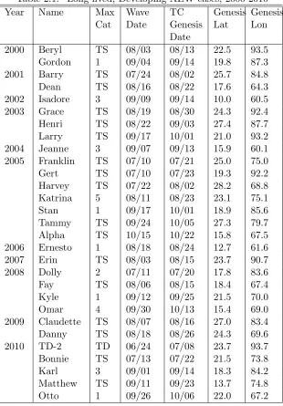
Between 2000 and 2010, the Atlantic Basin had 194 tropical cyclones, of which 29 formed from long-lived AEWs. Table 2.1 lists all 29 long-lived developing cases. Figure 2.1 shows the yearly percentage of tropical cyclones forming from long-lived waves. The 2005, 2008 and 2010 hurri-cane seasons experienced an above average number of tropical cyclones forming from long-lived AEW, at about 23%, while the 2002, 2004, 2006 and 2007 seasons each only had 1 tropical cyclone that formed from a long-lived AEW.
When examining the tracks of TCs that formed from long-lived waves (Figure 2.2), it is apparent that these storms are more likely to pose a threat to land. These storms are form-ing at a closer proximity to land makform-ing it more difficult to re-curve without makform-ing landfall. The statistics for the 11 hurricane seasons from 2000 to 2010 show 53% of all Atlantic trop-ical cyclones made landfall and by removing the long-lived AEW cases this number drops to 41%; however, of the 29 tropical cyclones that formed from long-lived waves, 79% made landfall.
Despite many of these TCs forming within close proximity to land, figure 2.3 shows there is no preference for TCs forming from long-lived AEWs to be stronger or weaker than TCs that do not form from long-lived AEWs. A t-test showed no statistical difference between the distribution of intensities for storms forming from long-lived AEWs and those that did not.
cre-ates a problem from a forecasting perspective as well as an emergency manager and public awareness perspective.
2.4
Observational Study
The observational study suggests there are likely two main mechanisms for maintaining AEWs. The first is through a PV flux into the wave from either mid-latitude sources or from other tropical disturbances and second is through convective generation of PV middle troposphere, due to the convective heating profile within the wave. However, the merger of a long-lived AEW with a mid-latitude or tropical PV source was rare, accounting for only 3 of the 29 cases. Instead, convection within the wave is linked to maintaining or intensifying a wave, while a lack of convection is linked to a decaying wave.
2.4.1 PV Basics
PV is used to track and describe the evolution of the waves in the study because it is a conserved quantity for insentropic, adiabatic processes. PV describes the combination of vorticity and stability as is given by the following equation:
P V = 1
ρζ
a· ∇θ (2.1)
where ρ is the density of the fluid, ζ a is the absolute vorticity, and ∇ θ is the gradient of potential temperature (Haynes and McIntyre 1987)
2.4.2 PV Flux into the Wave
the mid-latitude PV source catching up to, and merging with the AEW. Although part of the mid-latitude source continues to propagate past the AEW, the merger contributes to increasing PV within the wave. Four days after the merger the TC develops, denoted by the ”X” on the Hovmoller.
The interaction between the mid-latitude PV source and the wave is favorable, and leads to a rejuvenation of the wave and to a tropical cyclone several days later. However, in all three cases the merger with the mid-latitude PV source did not occur until 90°W, 60°W, and 50°W, respectively. Both pre-Erin and pre-Kyle had already met the criteria for a long-lived AEW, while pre-Omar was just 10° short of making it to the 60°W cutoff. These cases were already long-lived (or just about in the case of pre-Omar) even prior to the PV merger. While the mergers were important in reinvigorating the wave and likely helped lead to tropical cycloge-nesis, the mergers were not the main reason for supporting the wave as it crossed the tropical Atlantic. This suggests that the PV flux into the wave may not be the most common mecha-nism for maintaining long-lived AEWs.
It is also important to note difficulty in performing any PV budget calculation on the ERA-Interim data set, especially for a moving box surrounding the wave. The track of the waves in the reanalysis can be inconsistent in time and have sudden shifts in structure from one time to the next. Thus, quantifying the net flux of PV into or out of the wave-following box may not achieve the desired result, and may describe the variability in the reanalysis itself. Therefore, this study does not attempt to determine the contribution of the PV flux for each wave case, although in most cases it is assumed to be small. Visual inspection of the 29 cases only found 3 cases where the PV flux into the wave was an important part of the wave’s lifespan.
2.4.3 PV Generation from Convection: Case Studies
The convective generation of PV in the middle troposphere due to the convective heating profile within the wave is found to be the most important contributor to maintaining the long-lived AEWs. Examination of two long-lived AEW case studies shows an association between con-vective activity within the wave and an increasing or steady PV anomaly associated with the wave. Furthermore, weak or non-existent convective activity within the wave corresponds with a weakening PV anomaly associated with the wave.
the pre-Stan (2005) AEW is steady for the first 2 days at about 0.4 PVU before decreasing to 0.2 PVU by 23 September 2005. During this time of steady to decreasing PV anomaly, both the TRMM rainfall rate and the reanalysis vertical velocity are very small, indicating weak to no convection within the wave during this time. However, from 23 September until TC genesis on the 1 September, the PV anomaly associated with the AEW increases from about 0.2 PVU to about 0.55 PVU. During this time, the TRMM rainfall rate indicates bursts of convection within the wave. The ERA-Interim’s vertical velocity field represents this increase in convection as well.
Also in examining figure 2.6 for the pre-Ernesto (2006) AEW, a similar pattern is observed. Initially the PV associated with the wave is steady to decreasing from 18 August to 21 Au-gust. During this time, the TRMM rainfall rates and reanalysis omega field indicate weak and decreasing precipitation associated with the wave. However, on 20 August, both the TRMM rainfall rates and the reanalysis omega field indicate an increase in precipitation associated with the wave. The increase in precipitation rate precedes the increasing PV on 21 August.
Both of these examples show a relationship between convection associated with the wave and PV associated with the wave. The pre-Ernesto case points to the increasing convection occurring prior to the increase in PV since there is a delay from when the convection begins to when the PV begins to increase. The Stan case (figure 2.5) also shows the convection returning to the wave on on 23 September when the PV field is at a local minimum. It is only after the convection returns to the wave that the PV begins to recover. This observation is consistent with the second hypothesis, in that convective coupling with the wave may play a significant role in maintaining or strengthening the PV anomaly within the wave.
2.4.4 PV Generation from Convection: Extension to all Long-lived Devel-oping Cases
To study the differences between convectively active time periods and convectively inactive time periods for all waves, the TRMM precipitation rate was averaged in a 6°x 6°box around the wave center at every 6 hour reanalysis time for every wave. This procedure yields a time series of the precipitation rate for each wave. However, if all the times from all the waves are combined, then a distribution of the precipitation rates for all the cases is generated. From this distribution, threshold values for when convection is active versus when convection is inactive can be determined. Convectively inactive times were considered to be in the lower quartile of the distribution, and have precipitation rates of less than 0.14 mm day-1, while convectively
active times were considered to be in the upper quartile, and have precipitation rates greater than 0.73 mm day-1. The cut off values were visually checked with plan view plots of the TRMM precipitation and it was determined that the values meet the expectation for low convective activity and high convective activity, respectively. Once every convectively active and convec-tively inactive time was determine for all 29 cases, other variables were also area-averaged over the 6°x 6°box surrounding every wave at every time. Using the precipitation rate information, the convectively active and inactive times were used to separate the other variables to determine if there is a difference in the variables between the convectively active times and inactive times
A summary of the results can be seen in table 2.2. A t-test of each variable showed a statistically significant difference between the convectively active and inactive times. First, the relative humidity is, on average, higher at both 850 hPa and 600 hPa for the convectively active cases. Figure 2.7 (a) and (b) show the distributions for the relative humidity at 850 hPa and 600 hPa, respectively. The convectively active time periods (hatched) have a RH distribution that is bunched to the right of the graph, while the convectively inactive time periods (solid) have a distribution that has a longer tail toward lower RH values. This result shows that the ERA-Interim matches well with the TRMM precipitation field since the reanalysis should show higher RH at both levels when convection is observed to be active. This gives confidence in using the TRMM rainfall rate information to categorize convectively inactive and active times and separate the remaining variables.
convectively inactive wave is -0.107 PVU day-1, while the average tendency for a convectively active wave is 0.529 PVU day-1. Figure 2.7(d) shows the distribution of PV tendencies for the convectively active times is shifted to the positive PV tendencies while the distribution for the convectively inactive times is shifted to the negative PV tendencies. This statistic shows that over all 29 long-lived AEWs, the convectively active times are associated with increasing mid-level PV while the convectively inactive times are associated with decreasing PV.
The wind shear is counter-intuitive, with the convectively active time periods experienc-ing, on average, stronger wind shear than the convectively inactive time periods. It is hard to understand this result without further analysis, but the increased shear could be a result of the convection itself. The results suggest that for convection within waves, a small amount of wind shear may not be detrimental, even though it may not help with the organization of the wave. Dunkerton et al. (2009) even suggest that in the early stages of convective organization within the wave, the shear may play an important role in organizing the convection and making it longer lived. It is only when strong shear interacts with a mature vortex that it can be detrimental to the overall structure of the storm.
2.4.5 Case Study: Ernesto 2006
The purpose for examining the pre-Ernesto (2006) long-lived AEW is two fold. First, the case is studied extensively in the modeling study portion of the paper and so it is important to understand the evolution of the wave. Second, for the observational section of the paper, we examine the presence of a wave pouch as a possible mechanism for organizing convection within the wave and providing a pathway for convection to lead to wave maintenance.
Background
Atlantic Hurricane Ernesto (2006) formed from a long-lived AEW that emerged from the west coast of Africa on August 18th. The wave propagated across the Atlantic ocean for 7 days and spanned about 5000 km before becoming classified by the NHC as a tropical depression at 18Z on August 24th. Convection remained active within the wave for much of the time it crossed the Atlantic with only a few periods of weakened convection.
wave to the wave behind it that developed in TC Debby upon entering the Atlantic. Their study found that the Debby case exhibited stronger surface convergence, stronger upper-level divergence and higher relative humidity values than the pre-Ernesto case. All three of these parameters are very important in the bottom-up theory of tropical cyclogenesis and explain why the pre-Ernesto wave was not able to develop immediately upon entering the Atlantic. The increased wind shear associated with the SAL also kept the pre-Ernesto wave from becoming a stacked system for about 3-4 days after it moved off the African coast, while the pre-Debby wave was stacked almost immediately upon exiting the coast (Vizy and Cook 2009 and Zawislak and Zipser 2010). While the environmental conditions were not favorable for TC genesis for several days as the pre-Ernesto wave moved into the tropical Atlantic, the wave and its associated convection survived until the environmental conditions were favorable for TC genesis at 18Z August 24.
Wave Pouch Analysis
Examining the 600hPa relative flow along with the PV field in figure 2.8 suggests that the wave pouch may be a transient feature that is present only some of the time during the waves life span. The 18Z 18 August, 18Z 20 August and 18Z 24 August show a wave pouch while the remaining times show open flow through the wave. However, in examining each reanalysis time (not shown) the pouch appears and disappears at irregular intervals. The wave pouch should evolved smoothly as it depends on the wave speed and background flow speed which also evolve smoothly with time. The erratic nature of the pouch evolution with time in the ERA-Interim suggests that the reanalysis is not consistent in time with the low-amplitude, pre-Ernesto wave.
One key to understanding why the pouch does not vary smoothly in time comes in examin-ing the track of the wave (figure 2.9). The ERA-Interim had a hard time with the wave track as seen by the bunching of the track points for August 21 and August 22, indicating the wave was nearly stationary for a 24 hour period. Problems with the track speed in the reanalysis have a direct impact of the wave relative flow analysis as the wave pouch is sensitive to both the background wind speed and the translation speed of the wave. Since the track of the pre-Ernesto wave is not smoothly varying in time, it is no surprise that the wave pouch appears to come and go with time.
wave pouch suggests a mechanism for organizing convection within the wave and a pathway for upscale aggregation of vorticity. The difficulty in resolving the wave pouch for the pre-Ernesto case stresses the need for the high-resolution modeling study, which will more accurately de-scribe this sub-synoptic scale structure.
2.4.6 Conclusions from the Observational Study
The observational data available between the TRMM and ERA-Interim reanalysis suggest that the coupling of the AEW to convection may be key in maintaining or strengthening the wave. The population of long-lived AEW cases suggest that waves with strong convection are strength-ened while waves with weak to no convection are weakstrength-ened. However, the limitations of the ERA-Interim data set, in horizontal resolution, temporal resolution, and temporal consistency in wave structure prevent detailed calculations to better describe the important dynamical and thermodynamical processes.
The analysis of the pre-Ernesto wave shows a pouch structure may be present long before TC genesis. The favorable environment within the wave pouch, as described by Dunkerton et al. (2009), may be key to providing an area where convection is favored and can help sustain the parent wave. However, it is hard to have confidence in the exact structure of the pouch as described by the ERA-Interim reanalysis since this feature can be on a smaller scale than the wave itself. Also, variability in the ERA-Interim representation of the wave between reanalysis times gives little confidence in the temporal variability of the structure.
Table 2.1: Long-lived, Developing AEW cases, 2000-2010 Year Name Max
Cat Wave Date TC Genesis Date Genesis Lat Genesis Lon
2000 Beryl TS 08/03 08/13 22.5 93.5 Gordon 1 09/04 09/14 19.8 87.3 2001 Barry TS 07/24 08/02 25.7 84.8 Dean TS 08/16 08/22 17.6 64.3 2002 Isadore 3 09/09 09/14 10.0 60.5 2003 Grace TS 08/19 08/30 24.3 92.4 Henri TS 08/22 09/03 27.4 87.7 Larry TS 09/17 10/01 21.0 93.2 2004 Jeanne 3 09/07 09/13 15.9 60.1 2005 Franklin TS 07/10 07/21 25.0 75.0 Gert TS 07/10 07/23 19.3 92.2 Harvey TS 07/22 08/02 28.2 68.8 Katrina 5 08/11 08/23 23.1 75.1 Stan 1 09/17 10/01 18.9 85.6 Tammy TS 09/24 10/05 27.3 79.7 Alpha TS 10/15 10/22 15.8 67.5 2006 Ernesto 1 08/18 08/24 12.7 61.6 2007 Erin TS 08/03 08/15 23.7 90.7 2008 Dolly 2 07/11 07/20 17.8 83.6 Fay TS 08/06 08/15 18.4 67.4 Kyle 1 09/12 09/25 21.5 70.0 Omar 4 09/30 10/13 15.4 69.0 2009 Claudette TS 08/07 08/16 27.0 83.4 Danny TS 08/18 08/26 24.3 69.6 2010 TD-2 TD 06/24 07/08 23.7 93.7 Bonnie TS 07/13 07/22 21.5 73.8 Karl 3 09/01 09/14 18.3 84.2 Matthew TS 09/11 09/23 13.7 74.8 Otto 1 09/26 10/06 22.0 67.2
Table 2.2: Convectively Active vs Convectively Inactive Variable Convectively Inactive Convectively Active T-Test
RH 850 hPa 75.52 % 82.92 % 0 - Significant RH 600 hPa 58.59 % 73.92 % 0 - Significant PV 600 hPa 0.271 PVU 0.361 PVU 0 - Significant PV Tendency -0.107 PVU day-1 0.529 PVU day-1 0 - Significant
Wave M
id-La titu
de S our
ce
*
X
Chapter 3
Modeling Study
3.1
Modeling Study
3.1.1 High Resolution Model Simulation
To obtain a high resolution data set that is consistent with time, a WRF-ARW model simu-lation was run for the pre-Ernesto case (2006). The model has 28, terrain-following, vertical levels with the model top set at 50 hPa. Figure 3.1 shows the 2-domain configuration. A 12 km horizontal resolution outer domain encompasses the tropical Atlantic and spans the longitudes transversed by the long-lived pre-Ernesto AEW; and a 4 km moving nest that is initialized within domain 1, centered near 15°W, 10°N. The inner domain is defined to be about 20° lat-itude by 20°longitude to fully encompass the AEW and was prescribed preset moves to keep the domain centered on the pre-Ernesto AEW. The preset moves for the inner domain were originally defined by the anticipated translation speed of the wave from the ERA-Interim re-analysis. A test run was conducted to determine the approximate track of the wave in the 4km simulation and the preset moves were adjusted to keep the wave centered within the 4km domain.
The model was initialized from the ERA-Interim reanalysis on 0000 UTC 18 August 2010. The reanalysis data set was also used to update the boundary conditions on the 12 km grid every 6 hours. Sea surface temperature data was retrieved from the NCEP/MMAB real-time, global, sea surface temperature analysis (RTG SST). The RTG SST is a daily, half degree resolution data set that is derived from buoy, ship and satellite measurements. The daily sea surface temperatures were linearly interpolated to every 6 hours and were updated within the WRF model at that frequency.
closely reproduce the observed behavior of the pre-Ernesto wave. The observed case remained convectively active while it traversed the tropical Atlantic, before developing into a tropical depression by 1800 UTC 24 August 2006, as it entered the Caribbean Sea. The physics op-tions combination that most closely replicated the observed behavior was: the WRF Single-Moment 6-class microphysics scheme, the Rapid Radiation Transfer Model longwave radiation scheme, the Dudhia shortwave radiation scheme, the MM5 Similarity surface layer scheme, the NCEP/NCAR/AFWA Noah land surface model, the Yonsei University PBL scheme, and the Kain-Fritsch cumulus scheme on the 12 km domain with no cumulus parametrization on the 4 km domain. Also, the Garratt formulation for hurricane-specific surface fluxes (isftcflx 2) was used.
The goal of this study is not to determine the sensitivity of tropical cyclogenesis to micro-physics schemes, simply to generate a WRF simulation that closely reflects the observed case. This high resolution simulation will serve as a high quality data source to better understand the important processes in a long-lived AEW. However, it is intriguing that the microphysics scheme used in a simulation has such a profound impact on whether or not a wave develops into a tropical cyclone and how quickly it develops.
3.1.2 Model Verification
The simulation with the parametrizations described above performed remarkably well consid-ering the length of the simulation. The simulation was started at 0000 UTC on 18 August 2006 and was concluded at 0000 UTC on August 27 2006. The simulation is essentially a 9 day forecast, except the boundary conditions on the outer domain were updated by the ERA-Interm reanalysis, which provided information about the correct, large scale features to the outer model domain, and the SST was updated with the observed values.
Track Verification
distances traveled between 19 August and 20 August and 23 August and 24 August; however, the distances traveled each day in the WRF simulation are very consistent and any changes in speed are slow and continuous.
Intensity Verification
Also, by analyzing the mean sea level pressure with time (figure 3.3), the chosen simulation (line d) closely matches the overall intensity of the wave and the transition to a tropical cyclone. Two of the other WRF simulations developed sooner than observed (lines b and c), while the other simulation did not result in tropical cyclogenesis and the wave begins to dissipate by the end of the simulation (line a). From the 18th to the 22nd, the chosen WRF simulation closely matches the ERA-Interim (line e) semi-diurnal pressure fluctuations. On 22 August, a weak low level circulation develops in the WRF simulation and can be seen as a lowering of the pressure by about 5 hPa from the ERA-Interim reanalysis. The development of the low-level circulation, which is not captured by the ERA-Interim, indicates a regime change from a true AEW, which has a circulation concentrated in the mid-levels, to a pre-Wind Induced Surface Heat Exchange (WISHE, Emanuel 1986) disturbance. From 25 August 2006 to 27 August 2006 a continual drop in sea level pressure is observed in the WRF simulation, which is associated with tropical cyclogenesis, and closely reflects the observed drop in sea level pressure measured by the NHC (line f). Not surprisingly, the ERA-Interim reanalysis fails to capture the dropping central pressure between 25 August and 27 August and is likely because of the course 1.5° resolution failing to represent the newly forming tropical cyclone.
Precipitation Verification
Figure 3.4 shows a comparison between the precipitation fields as simulated by WRF (a) and as observed in the TRMM 3B42 data set (b), averaged over a two-day period from 0000 UTC 19 August 2006 to 0000 UTC 21 August 2006. The TRMM-observed precipitation field in figure 3.4(b) shows an observed precipitation band west of 20°W centered between 5°N and 10°N. The WRF simulation accurately places the observed precipitation band, but it is slightly stronger in intensity than observed, as indicated by the presence of more shading over 64 mm/day. West of 35°W the WRF simulated precipitation associated with the ITCZ is dis-placed north of the TRMM-observed precipitation.
Dur-ing the averagDur-ing time, the wave travels between about 37°W and 55°W and shows an overall northward shift in precipitation from the previous averaging time. The observed precipitation is centered near 10°N during the averaging period and transitions from weaker rain rates in the east, about 4 to 8 mm/day, to stronger rain rates in the west, greater than 32 mm/day in some locations. The weaker rain rates observed near 37°W indicates decreased convection with the wave around 0000 UTC 22 August 2006, before the convective activity increases in the following two days. The WRF simulation reflects the observed structure with the weakest precipitation intensity near 37°W, increasing toward the west. The main difference from the observed precipitation is the lack of precipitation over South America near 55°W in the WRF simulation. In the WRF simulation, the precipitation over the continent is displaced west of 60°W (not shown) with similar intensity to what is observed by the TRMM. This is of little concern for our study as the precipitation pattern directly related to the pre-Ernesto AEW appears consistent with observation.
Figure 3.4 (e) and (f) shows the WRF simulation and TRMM-observed precipitation rate (mm/day) averaged between 0000 UTC 25 August 2006 and 0000 UTC 27 August 2006, days 8 and 9 of the simulation. Remarkably, the WRF simulated precipitation pattern (figure 3.4(e)) closely matches the observed precipitation pattern (figure 3.4(f)). The primary area of interest is the precipitation over the Caribbean, which is associated with the developing tropical cyclone in both the observed and simulated cases. The WRF simulation tracks the wave slightly faster than observed, spanning from about 62°W to 75°W, while the observed precipitation is shifted eastward, spanning from about 60°W to 73°W. This agrees with the track information from figure 3.2, which shows the WRF simulation placing Ernesto about a degree farther west than the NHC best track data. The WRF simulation is slightly wetter than observed but captures the structure well, even capturing the northward track of the storm on day 9 of the simulation.
Verification Conclusions
3.2
Modeling Results
3.2.1 Wave Evolution and Wave Pouch Analysis Wave Pouch Evolution
Following Dunkerton et al. (2009), the wave is analyzed from a Lagrangian frame of reference, with the wave motion subtracted from the total flow. The wave speed is estimated from the Hovmoller diagram in figure 3.6, where the 850 hPa v-wind is averaged between 7°N and 17°N. The analysis shows an initial wave speed of about 8.6 ms-1until 20 August, when it speeds up to
about 11 ms-1before slowing to about 7.11 ms-1on 24 August. These wave speed estimates are then subtracted from the total u-wind component, resulting in a wave relative frame of reference.
Figure 3.7 shows the evolution of the wave pouch at several levels throughout the simula-tion. The wave pouch is well defined above 700 hPa by 00Z August 20 (48 hours), but shows a northward tilt at 850 hPa and no closed pouch at 925 hPa. This structure mates well with the observation in previous studies (Vizy and Cook 2009 and Zawislak and Zipser 2010), where the equatorward tilt with height persisted for a few days over the Atlantic due to the vertical shear associated with the SAL. By 00Z August 22 (96 hours) the wave pouch is well defined at all levels, which corresponds well to the time when the surface circulation develops. Shortly after this time, the wave encountered vertical wind shear, subsidence and drying in the upper levels. The effects of the synoptic scale influence can be seen at the 350 hPa level, where the pouch has given way to streamlines that flow directly through the wave. However, the pouch remains stacked and disturbed below 500 hPa. By 00Z August 26 the vorticity in lower troposphere has become concentrated in the center of the wave pouch, showing a contraction in scale from earlier time frames. The contraction in scale shows a merger of smaller scale vorticity maxima with time as the system moves toward TC genesis, consistent with the upscale aggregation of PV shown in the bottom-up pathway for TC genesis.
Wave Pouch and Relative Humidity
Figure 3.9 shows the evolution of the wave pouch and relative humidity field at 700 hPa. For the first 72 hours the wave pouch is surrounded by fairly moist air (generally great than 60% humidity). However, by 00Z 23 August (figure 3.9(e)) very dry air, near 30% RH, is in place on the north side of the wave. However, by examining the wave-relative streamlines, we can see that wave pouch protects the air inside from the dry air. The air near the center of the wave pouch is repeatedly recirculated and not exposed to the outside dry air, allowing it to remain more moist than the environmental air. By 00Z 24 August (figure 3.9) some of the dry air from the northern side of the wave has been advected around the south side of the wave, but the air within the center of the wave pouch remains moist.
The evolution of the RH field at the 350 hPa level (figure 3.10) is different from the 700 hPa evolution. A pouch structure develops at 350 hPa by 00Z August (48 hours), indicating that the wave has developed some vertical extent into the upper troposphere and that the mean wind speed at that level closely matches the translation speed of the wave. The pouch structure at this level helps to protect the center of the wave from dry air intrusions, since the very dry air (less than 10% RH) to the north and west is directed around the center of the wave. However, by 00Z 23 August (120 hours) the pouch breaks down as the upper level background wind speed increases and shears the wave. This allows the very dry air from the west to intrude the wave. The dry air intrusion in the upper levels can also be seen in the height-time plot (figure 3.11(c)). The dry air is associated with synoptic subsidence that inhibits the convection on the western half of the wave (as can be see in figure 3.8(e)).
Height-time Analysis of the Wave Pouch
minor disruption in the strong convective divergence profile, with a weakening of the surface convergence and a weakening of the strong divergence aloft. This disruption occurs concur-rently with a stabilization (neither increasing or decreasing) in the mid-level vorticity and PV maxima. Between 72 hours and 96 hours, the deep convective divergence profile returns, along with the deep convective diabatic heating profile. With a return of the deep convective heating profile, the PV and vorticity fields begin to strengthen and descend from the mid-levels again, showing that the convection is key to supporting the parent wave.
Between 96 hours and 126 hours, the strongest vorticity and PV signature is located near the top of the boundary layer, and much lower than what is expected for a pure AEW. The development of vorticity near the surface is consistent with a low-level circulation that devel-ops about 96 hours into the simulation, indicating that the wave has begun to transition to a pre-WISHE disturbance. Not long after the surface circulation develops, about 102 hours into the simulation, the mid-level vorticity begins to weaken. The weakening of the mid-level vorticity coincides with very dry air intruding on the wave pouch between 400 hPa and 250 hPa (3.11(c)). Also during this time, the divergence profile (3.11(d)) is no longer representative of deep convection as the level of maximum divergence is located in the mid-troposphere. The disruption in the convective heating profile can also be seen in the diabatic heating (3.11(e)) as the level of maximum heating is confined below 500 hPa. This shows that the large scale subsidence suppresses the convection within the wave, which leads to a weakening of the parent wave, which is seen in the weakening vorticity and PV fields.
After 126 hours, the divergence and diabatic heating transition back to a deep convective profile. The low level vorticity and PV stop decreasing and stabilize through about 180 hours. The relative humidity begins to slowly increase above 500 hPa after the deep convective profile returns to the wave pouch, thus implying the return of deep convection within the wave helps to moisten the upper levels of the troposphere. The convective heating profile appears to be es-sential in maintaining or strengthening the wave; however, the PV and vorticity budgets in the following sections help reveal the pathway through which this mechanism works to strengthen the wave.
suggests a vertical development of the vortex into the upper troposphere. This sequence seems to fit the bottom-up theory for tropical cyclogenesis, where the low level vorticity is stretched and advected upward, creating a deep, coherent vortex that becomes the tropical cyclone.
Wave Pouch Analysis Conclusions
The height-time cross sections show an association between convection within the wave and a maintaining or strengthening wave. When the convection becomes suppressed within the wave, the wave scale vorticity and PV decreases. The convection within the wave pouch promotes diabatic heating in the middle troposphere, convergence in the lower to mid-troposphere and divergence in the upper troposphere. This supports the findings of Dunkerton et al. (2009), where the wave pouch is characterized by a convective heating profile, enhanced RH and en-hanced vorticity.
The wave pouch analysis also shows the presence of a pouch between 500 hPa and 700 hPa from 24 hours to 216 hours (the end of the simulation). A deep pouch (500 hPa to 925 hPa) develops by 96 hours or about 4 days prior to TC genesis. The presence of this pouch in the lower troposphere likely helps to ensure the integrity of the wave when it experiences the detrimental effects of synoptic scale subsidence. After the interaction with the upper level dry air and subsidence, the wave pouch in the lower troposphere still provides a favored region for convection and aggregation of vorticity. This time series also suggests that convective coupling may be key to maintaining or strengthening the mid-level and low-level vorticity; however the direction of causality is hard to infer from these plots and will be examined more closely in the PV and vorticity budget sections that follow.
Dunkerton et al. (2009) only discuss the importance of the pouch within a few days prior to TC genesis, while this case study shows this structure may exist long before TC genesis begins. The wave pouch persists for 7 days prior to tropical cyclogenesis and may be an important mechanism for protecting the convection within the wave. The pouch may also help cascade energy from the mesoscale storm features to the synoptic scale wave due to the enhanced cy-clonic vorticity and weak deferomation.
3.2.2 Potential Vorticity Budget
and adapted to a storm-following form by Kieu and Zhang (2009). Kieu and Zhang (2009) formulate the PV budget equation from Haynes and McIntyre (1987) into a volume averaged form, which allows for a time series analysis of the budget in a storm following format; and is written as:
d dt
Z
V(t) qdV
! =
Z
V(t)
(q∇ ·u)dV + Z
V(t)
ω· ∇H
ρ dV (3.1)
+ Z
V(t)
∇ ·(F× ∇θ)
ρ dV +
Z
S(t)
q(U−u)·ndS
where q is the potential vorticity, u is the full 3D wind field, ω is the 3D absolute vorticity, H is the diabatic heating rate, F is the 3D frictional force, U is the speed of the boundaries and ∇is the 3D gradient operator. This formulation of the PV budget states that the volume
averaged time rate of change of PV is described by the terms on the right hand side. Those terms are, from left to right, the 3D divergence of PV or stretching term, the diabatic PV production term, the frictional generation/destruction term and the across boundary PV flux. To make the computation easier, it should be noted that the across boundary PV flux term can be rewritten using Gauss theorem, which states that a surface flux can be written in terms of the volume integral of the divergence within the enclosed region. Rewriting the last term yields:
d dt
Z
V(t)
qdV
! =
Z
V(t)
(q∇ ·u)dV + Z
V(t)
ω· ∇H
ρ dV (3.2)
+ Z
V(t)
∇ ·(F× ∇θ)
ρ dV +
Z
V(t)
∇ ·(qU)− ∇ ·(qu)dV
d dt
Z
S(t) qdS
! =
Z
S(t)
(q∇ ·u)dS+
Z
S(t)
ω· ∇H
ρ dS (3.3)
+ Z
S(t)
∇ ·(F× ∇θ)
ρ dS
+ Z
S(t)
(∇ ·(qU)−q∇ ·u−uh· ∇hq)dS
+ Z
S(t)
−
dwq dz
dS
where uh is the horizontal components of the wind, ∇h is the 2D gradient operator and w is
the z-direction wind speed. This formulation of the PV budget shows that the time rate of change of area average PV on a height surface can be explained by the terms on the right hand side. The first three terms on the right hand side of the equation are the same as in equation (1) except that instead of volume averaging the terms are averaged at each height surface, thus retaining the budget information in the vertical. For clarity, the boundary term is broken into two terms, the first describes the net flux of PV across the lateral boundaries of the height surface, while the second term is the area average vertical flux of PV. It is im-portant to separate the vertical flux from the boundary term in the area average context so that it is possible to distinguish between PV being fluxed into or out of the area of interest and PV that is within the area of interest but is moving between height levels due to vertical motion.
The PV budget is calculated using the output from the 4-km model domain at 12 minute intervals. Before plotting the height-time cross sections of the PV budget a 1-hour running average is applied to the fields to help eliminate some of the high-frequency noise in the compu-tation. The friction term is ignored in this study since the focus is on levels above the boundary layer, specifically in the middle troposphere. The center of the wave pouch is recorded every 6 hours and is interpolated to a 12-minute position for centering the PV budget box for area or volume averaging. The speed of the lateral boundaries (U) is calculated from the centered difference of the 12 minute positions.
the total derivative of theta (Dθ
Dt) at each time and subtracting the 3D theta advection (−u·∇θ).
In doing so, it is assumed that any changes in theta not accounted for by advection are diabatic heating tendencies. In theory, this method should be more accurate as it automatically includes numerical diffusion, mixing and frictional effects, which cannot be read from the WRF output. To check that this method accurately describes the diabatic heating tendency, it was compared to the diabatic heating tendency read directly from the WRF file. The comparison showed the two methods to be almost identical, except near the melting level where some minor differences appeared. Calculating the PV budget with the calculated diabatic heating term eliminated the residual problems centered on the melting level, and improved the overall accuracy of the PV budget calculation.
3.2.3 Potential Vorticity Budget Analysis
Figure 3.12 shows the results from the PV budget in height-time format for easy comparison with figure 3.11. All terms are area averaged at each height level over a 440 km x 440 km box centered on the wave pouch. To better understand how the mid-troposphere potential vorticity anomaly is maintained, evolves and descends to the surface, each term of the potential vorticity budget must be carefully considered at all phases in the evolution of the wave. First a general overview of the budget will be discussed with the aid of the height-time plots, followed by a more careful analysis of each phase in the evolution using time-averaged profiles of the budget and linking that information back to the meteorological conditions during each phase.
Divergence Term Overview
Diabatic + Vertical Flux Term Overview
The diabatic tendency term and vertical flux term have been added together for presentation in the height-time format (figure 3.12(c)) but will be displayed independently in the next section of time-average vertical profiles. It is easier to understand the the net effect of the diabatic term and vertical flux term when they are are combined since the terms are generally equal and opposite in sign. The diabatic tendency is typically positive in the lower troposphere and negative in the upper troposphere due to the deep convective diabatic heating profile. Since the maximum level of heating is in the mid-troposphere, this acts to add static stability to the lower portion of the atmosphere and decrease the static stability of the upper portion of the atmosphere. By definition, PV can be increased by increasing the static stability, thus the PV tendency due to the diabatic heating profile should be positive below the level of maximum heating.
Conversely, the vertical flux term is largely negative in the lower troposphere and positive in the upper troposphere, opposite to the diabatic term. This pattern is explained by the ver-tical flux divergence of PV in the low-levels, where it is being diabaver-tically gnerated, and flux convergence in the upper levels. Therefore, the vertical flux of PV and the diabatic generation of PV are nearly in a steady state. Thus, since the patterns largely cancel, more information can be gathered from the net effect of the two, offsetting processes. With these two processes combined, we find that the net effect of the vertical flux and diabatic heating is generally a nega-tive PV tendency in the mid-troposphere, generally acting in opposition to the divergence term.
Boundary Term Overview
The boundary term (figure 3.12(d)) is generally much smaller than the preceding terms. This should be the case since the averaging box is designed to contain the bulk of the PV anomaly associated with the wave, and thus only very small fluxes should occur through the edges of the box. However, if the fluxes through the side of the box are larger than their typical near-zero val-ues it can be interpreted as a flux into or out of the wave itself due to the careful placement and size of the averaging box. Throughout the simulation, the boundary term is largely near-zero except for a few time frames where some stronger negative tendencies are seen in the mid-levels.
Residual Term Overview
at-tributed to frictional affects. The negative tendency due to friction is especially more noticeable once the low-level circulation forms just after 96 hours. Also, once the convection becomes in-creasingly active in the wave, after 120 hours, there is a net positive tendency that appears in the residual term in the mid-troposphere, but this is still smaller than the leading terms of divergence, diabatic heating and vertical flux. Overall, the residual term does not discredit the usefulness of the PV budget terms in finding some understanding about dynamics and thermo-dynamics of the AEW and its transition to a tropical cyclone.
PV Budget Evolution
Between hours 24 and 96 the mid-level PV associated with the wave increases from about 0.5 PVU to 0.9 PVU. The PV is also descending with time and the low-level PV continues to increase.
The divergence term (figure 3.12(b)) is mainly positive throughout this period of PV maintenance and strengthening. The divergence term is positive throughout much of the troposphere suggesting that diabatic heating is working to decrease the mass within the volume and contributing to the overall concentration of PV, leading to a positive PV tendency.
The diabatic / vertical flux term (figure 3.12)(c) is primarily negative throughout the depth of the troposphere, but especially in the low to mid levels.
The boundary term (figure 3.12(e)) is mainly small and noisy compared to the preceding terms, with the exception of shortly after 72 hours in the mid and upper troposphere. Shortly after 72 hours, only the boundary term can account for the negative PV tendency in the mid to upper levels, which suggests a flux of higher PV air out of the wave and lower PV air into the wave.
The time-averaged PV budget profile (figure 3.13(a)) for hours 24 to 96 confirms the find-ings of the height-time plot analysis. The main contributor to the positive PV tendency in the middle and lower troposphere is the divergence term. Here we can see the opposing effects of the diabatic and vertical flux terms, and when compared to the height-time plot it is easy to see how the terms add up to be overall negative throughout much of the troposphere. Also from this time-average perspective, the boundary term is indeed much smaller than the leading terms.
the mid level PV decreasing from about 0.9 PVU to about 0.6 PVU.
The strong mid-level diabatic heating tendency (figure 3.11(e)) is weakened and becomes concentrated in the lower-levels. The divergence profile (figure 3.11(d)) shows the disrup-tion of the deep convective heating profile by the loss of strong divergence in the upper troposphere, and the change from weak convergence to weak divergence in the mid levels.
In the mid-levels, the positive tendency of the divergence term becomes very weak com-pared to the negative tendency of the diabatic / vertical flux term and the boundary term, and so an overall decrease in the PV is observed.
The boundary term is very important in decreasing the mid and upper level PV as low PV air enters the wave while interacting with the large scale subsidence.
Since the divergence term is still largest in the boundary layer and the diabatic / vertical flux term becomes positive in the boundary layer, the low-level PV is maintained.
The time-averaged PV budget profile (figure 3.13(b)), for hours 96 to 126, reflects the analysis of the height-time plot.
The divergence term is very weak but still positive and the diabatic / vertical flux term is weak but still negative. The boundary term describes the decrease in mid-level PV well as the wave interacts with large scale subsidence during this time period.
The suppression of the deep convective heating profile inhibits concentration of PV, thus limiting the only term that can provide a significant PV source for the wave.
Hours 126 to 192 of the simulation illustrate a rejuvenation of the deep convective heating profile (figure 3.11(e)) along with a strengthening and maintenance of the PV associated with the pre-depression.
The divergence term is the dominate positive tendency term throughout the depth of the troposphere, while the diabatic / vertical flux term is the dominate negative tendency term.
Figure 3.13(c) shows that even the boundary term contributes negatively to the mid-level PV during this period.
The only term responsible for the strengthening and maintenance of the wave is the divergence term, which relies on the deep convective heating profile.
and the boundary term becomes less negative. Figure 3.13(d) shows that the divergence term is the leading positive contributor to the total PV especially near the surface, and best explains the increase of PV throughout the depth of the troposphere. Since the divergence term did not strengthen from prior times, tropical cyclogenesis may have been the result of the boundary term and the diabatic / vertical flux becoming less negative.
This confirms that long-lived waves may be a result of processes that both support the wave and inhibit the wave. Here, the wave is maintained through convection within the wave pouch, but upper-level shear and subsidence are enough to prevent tropical cyclogenesis. The balance between these competing processes allows the wave to be maintained without developing.
3.2.4 Vorticity Budget
To further support the PV budget analysis and to provide more insight into the dynamics of the AEW, a vorticity budget is calculated following Haynes and McIntyre (1987), Kieu and Zhang (2009), and Wang et al. (2010a). The flux form of the vorticity equation in isobaric coordinates is written as:
∂η
∂t =−∇ · u
′η
− ∇ ·
−ωk×du
′
dp
+Solenoid+F riction (3.4)
where η is the 2D absolute vorticity calculated using the wave relative winds, u’, andω is the pressure coordinate vertical velocity. Consistent with the previous studies, the solenoid and friction terms are assumed to be small when compared to the leading terms and are thus not included in the calculation. The solenoid term will only be active where there are large density and temperature differences which are not typically found in the tropics and the friction term will be small except in the boundary layer, which is of little concern to understanding vorticity tendencies in the middle troposphere. The first term on the right hand side is the flux diver-gence of vorticity, which combines the horizontal advection into or out of the area averaging box and stretching in the vertical. The second term is a combination of tilting horizontal vorticity into the vertical and the vertical advection of vorticity. The tilting portion of second term is considered to be small due to generally weak wind shear in the tropics and thus the vertical advection will dominate this second term.