University of Windsor University of Windsor
Scholarship at UWindsor
Scholarship at UWindsor
Electronic Theses and Dissertations Theses, Dissertations, and Major Papers
1-1-2007
On the implementation and refinement of outerplanar graph
On the implementation and refinement of outerplanar graph
algorithms.
algorithms.
Tao DengUniversity of Windsor
Follow this and additional works at: https://scholar.uwindsor.ca/etd
Recommended Citation Recommended Citation
Deng, Tao, "On the implementation and refinement of outerplanar graph algorithms." (2007). Electronic Theses and Dissertations. 6972.
https://scholar.uwindsor.ca/etd/6972
On th e Im plem entation and R efinem ent o f
O uterplanar Graph A lgorithm s
by
Tao Deng
A Thesis
Submitted to the Faculty of Graduate Studies through Computer Science
in Partial Fulfillment of the Requirements for the Degree of Master of Science at the
University of Windsor
Windsor, Ontario, Canada 2007
Library and Archives Canada
Bibliotheque et Archives Canada
Published Heritage Branch
395 W ellington Street Ottawa ON K1A 0N4 Canada
Your file Votre reference ISBN: 978-0-494-34997-7 Our file Notre reference ISBN: 978-0-494-34997-7 Direction du
Patrimoine de I'edition
395, rue W ellington Ottawa ON K1A 0N4 Canada
NOTICE:
The author has granted a non exclusive license allowing Library and Archives Canada to reproduce, publish, archive, preserve, conserve, communicate to the public by
telecommunication or on the Internet, loan, distribute and sell theses
worldwide, for commercial or non commercial purposes, in microform, paper, electronic and/or any other formats.
AVIS:
L'auteur a accorde une licence non exclusive permettant a la Bibliotheque et Archives Canada de reproduire, publier, archiver,
sauvegarder, conserver, transmettre au public par telecommunication ou par I'lnternet, preter, distribuer et vendre des theses partout dans le monde, a des fins commerciales ou autres, sur support microforme, papier, electronique et/ou autres formats.
The author retains copyright ownership and moral rights in this thesis. Neither the thesis nor substantial extracts from it may be printed or otherwise reproduced without the author's permission.
L'auteur conserve la propriete du droit d'auteur et des droits moraux qui protege cette these. Ni la these ni des extraits substantiels de celle-ci ne doivent etre imprimes ou autrement reproduits sans son autorisation.
In compliance with the Canadian Privacy Act some supporting forms may have been removed from this thesis.
While these forms may be included in the document page count,
their removal does not represent any loss of content from the thesis.
Conformement a la loi canadienne sur la protection de la vie privee, quelques formulaires secondaires ont ete enleves de cette these.
A bstract
An outerplanar graph is a graph that can be embedded on the plane such that all the vertices lie on the exterior face and no two edges intersect except possibly at a common end-vertex. Five sequential algorithms had been proposed for rec ognizing outerplanar graph in the literature and all run in linear time and space. Although among them, the algorithms of Mitchell, Wiegers, and Tsin and Lin are obviously superior, no efforts had been made in comparing their performances during run-time.
In this thesis, the aforementioned three algorithms are implemented and their performances are compared using a large number of randomly generated graphs. Furthermore, the algorithms of Mitchell and Wiegers are modified so that an out- erpalnar embedding is generated if the input graph is outerplanar. Correctness proofs of the modification are presented. It is also shown that the complexity of the modified algorithms remain linear in both time and space.
A cknow ledgm ents
I would like to express my sincere gratitude to my supervisor Dr. Tsin whose guidance and encouragement helped me during the research. His attitude of pro viding only high quality work, has made a deep impression on me. Besides of being an extrordinary supervisor, Dr. Tsin is a dear friend to me. I feel so lucky to get to know Dr. Tsin in my life.
I wish to express my thanks to my thesis committee members, Dr, Wu, Dr. Kao and Dr. Ahmad who used their precious time and provided invaluable suggestions to my thesis.
C ontents
A bstract iii
Acknowledgm ents iv
List o f Figures vii
List o f Tables x
1 Introduction 1
1.1 M otivation... 1
1.2 Thesis S ta te m e n t... 4
1.3 Organizations of T hesis... 4
2 Background 6 2.1 Basic D efinition... 6
2.1.1 Related C o n ce p ts... 6
2.2 Representation of G r a p h ... 10
2.2.1 Adjacency M a trix ... 10
2.2.2 Adjacency List ... 10
2.3 Graph Traversing Techniques ... 11
2.3.1 Depth First S e a r c h ... 11
2.4 Planar Graphs and Outerplanar Graphs ... 14
2.4.1 Planar G r a p h ... 14
2.4.2 Outerplanar G r a p h ... 15
2.5 Bucket S o r t ... 16
3 A Study of M itchell’s Algorithm 17 3.1 Maximal Outerplanar Algorithm... 17
3.2 Outerplanar a lg o rith m ... 18
3.3 An Example of Mitchell’s Outerplanar A lg o rith m ... 19
3.3.1 Removal of 2-v ertices... 20
3.3.2 Bucket S o r t ... 22
CONTENTS CONTENTS
3.4 Im plem entation... 24
3.4.1 Our strategies in the im plem entation... 24
3.4.2 Main Steps of our Implementation... 25
3.4.3 A Detailed Implementation ... 26
3.4.4 An Illustration of Mitchell’s Outerplanar Algorithm . . . . 30
4 A Study of W iegers’ Algorithm 33 4.1 Outerplanar a lg o rith m ... 33
4.1.1 The 2-Reducible Graph Algorithm ... 33
4.1.2 The Edge Coloring T e ch n iq u e... 36
4.2 Im plem entation... 40
4.2.1 An E xam ple... 43
5 A Study o f Tsin and Lin’s Algorithm 47 5.1 Outerplanar a lg o rith m ... 47
5.2 An Example of Tsin and Lin’s Outerplanar Algorithm... 50
5.3 Im plem entation... 52
6 Experim ents 55 6.1 Experimental D a t a ... 55
6.1.1 The Input Graphs ... 55
6.1.2 Experimental R esu lts... 56
6.2 D iscussion... 57
7 Em bedding of Outerplanar Graphs 60 7.1 A Modified Mitchell’s Algorithm for Outerplanar Embedding . . . 60
7.2 Proof of Correctness ... 65
7.3 An E x am p le... 66
7.4 A Modified Wiegers’s Algorithm for Outerplanar Embedding . . . 69
8 Conclusions 70
Bibliography 71
List of Figures
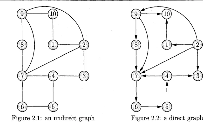
2.1 an undirect g r a p h ... 7
2.2 a direct g r a p h ... 7
2.3 A spanning tree of the graph in Figure 2 .1 ... 8
2.4 # 5 ... 9
2.5 # 4 ... 9
2.6 # 3,3 ... 9
2.7 # 2,3 ... 9
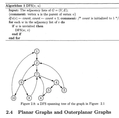
2.8 a DFS spanning tree of the graph in Figure 2 . 1 ... 14
3.1 An Illustration of Mitchell’s A lg o rith m ... 20
3.2 An Illustration of Mitchell’s Algorithm: after removal of node 5 . 20 3.3 An Illustration of Mitchell’s Algorithm: after removal of node 4 . 21 3.4 An Illustration of Mitchell’s Algorithm: after removal of node 3 . 21 3.5 An Illustration of Mitchell’s Algorithm: after removal of node 6 . 22 3.6 An Illustration of Mitchell’s Algorithm: P A IR S and E D G E S after all the 2—vertices are rem oved... 22
3.7 An Illustration of Mitchell’s Algorithm: P A IR S and E D G E S be fore Bucket S o r t... 23
3.8 An Illustration of Mitchell’s Algorithm: P A IR S and E D G E S after one-pass Bucket S o r t ... 23
3.9 An Illustration of Mitchell’s Algorithm: P A IR S and E D G E S after a two-pass Bucket S o r t ... 24
3.10 An Illustration of Mitchell’s Outerplaner Algorithm; | V\ = 6. . . . 30
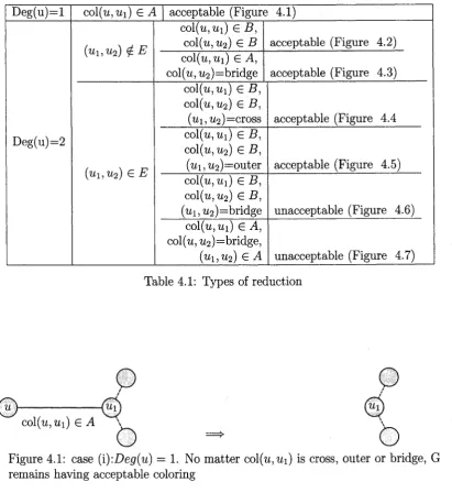
3.11 An Illustration of Mitchell’s Algorithm: After removal of vertex 5 31 3.12 An Illustration of Mitchell’s Algorithm: After removal of vertex 4 31 3.13 An Illustration of Mitchell’s Algorithm: After removal of vertex 3 32 3.14 An Illustration of Mitchell’s Algorithm: After removal of vertex 6 32 4.1 case (i):Deg{u) — 1. No matter col(u,Ui) is cross, outer or bridge, G remains having acceptable coloring... 37
4.2 case (ii):Deg(u) = 2, U\ and u2 are not joined with an edge. . . . 38
4.3 case (iii)\Deg(u) = 2, U\ and u2 are not joined with an edge. . . 38
4.4 case (iv):Deg(u) = 2, ui and u2 are joined with an edge... 39
4.5 case (iv)\Deg(u) = 2, u\ and u2 are joined with an edge... 39
4.6 case (v):Deg(u) = 2, u\ and u2 are joined with an edge... 40
LIST OF FIGURES LIST OF FIGURES
4.8 Example of Implementation of Wiegers’ Algorithm: a graph with
6 vertices ... 44
4.9 Example of Implementation of Wiegers’ Algorithm: u — 4 ... 44
4.10 Example of Implementation of Wiegers’ Algorithm: u = 5 ... 45
4.11 Example of Implementation of Wiegers’ Algorithm: u = 3 ... 45
4.12 Example of Implementation of Wiegers’ Algorithm: u = 3 ... 46
4.13 Example of Implementation of Wiegers’ Algorithm: u = 3 ... 46
4.14 Example of Implementation of Wiegers’ Algorithm: u = 3 ... 46
5.1 a DFS spanning tree of the graph in Figure 2 . 1 ... 50
5.2 non-trivial path P \ ... 51
5.3 trivial path P2 ... 51
5.4 non-trivial path P s... 51
5.5 non-trivial path P i... 51
5.6 non-trivial path P5 ... 51
6.1 The performances of the three algorithms on all graphs, as a func tion of the graph s i z e ... 57
6.2 The performances of the three algorithms on Outerplanar Graphs, as a function of the graph s i z e ... 58
6.3 The performances of the three algorithms on non-Outerplanar Graphs, as a function of the graph s i z e ... 59
7.1 Example of OuterPlanar Embedding (Mitchell’s Algorithm) . . . 66
7.2 Example of OuterPlanar Embedding (Mitchell’s Algorithm): after removal of vertex 5 ... 67
7.3 Example of OuterPlanar Embedding (Mitchell’s Algorithm): after removal of vertex 4 ... 67
7.4 Example of OuterPlanar Embedding (Mitchell’s Algorithm): after removal of vertex 1 ... 68
List of Tables
2.1 Adjacency matrix of the graph in Figure 2 .1 ... 10
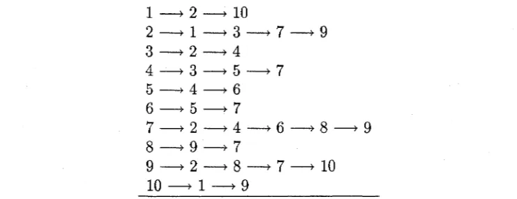
2.2 Adjacency lists of the graph in Figure 2 . 1 ... 11
List of Algorithms
1 DFS(w, u ) ... 14
2 Bucket Sort {Array, n) ... 16
3 An Implementation of Mitchell’s Outerplanar A lg o r ith m 27 4 Check the adjacency list of vertex a for vertex b ... 28
5 Add White N o d e ... 28
6 Add Red Node ... 29
7 Remove Red Node ... 29
8 Check if PAIRS C E D G E S ... 30
9 2-Reducible Graph A lg o rith m ... 35
10 Implementation of Wiegers’ Outerplanar Graph Algorithm . . . . 41
11 M oveEdge... 42
12 Tsin and Lin’s Outerplanar Algorithm [50]... 50
13 Random biconnected G rap h s... 56
14 Modified Mitchell’s Outerplanar A lgorithm ... 63
15 Check the adjacency list of vertex a for vertex b ... 64
16 Add White v e rte x ... 64
C hapter 1
In trod u ction
A general definition of graph is any mathematical object involving nodes and connections between them. Graph-theoretic problems occur naturally in a great diversity of applications, such as electrical circuits, organic molecules, ecosystems, sociological relationships, databases, and in the flow of control in a computer pro gram.
1.1
M otivation
An outerplanar graph is a graph that can be embedded in the plane so that all the vertices lie on the boundary of the exterior face and no two edges cross each other. Outerplanar graphs appear naturally in a wide variety of applications. For instance, in RNA structure, every secondary structure which consists of a list of base pairs has the structure of an outerplanar graph [52]. In computer networks, message routing is generally an expensive task in terms of time and space complex ity. However, for outerplanar network, compact routing schemes [21] and compact fault-tolerant message routing method [21] had been developed. Although in real- life situation, computer networks are usually planar, Frederickson showed that the problem of designing efficient compact routing scheme for planar networks can be reduced to that for a class of outerplaner networks satisfying certain prop erties [20]. Furthermore, Gongalves recently showed that every planar graph can be decomposed into two outerplanar subgraphs [25]. The study of outerplanar network thus plays an important role in message routing.
1.1 Motivation
and NP-hard, respectively, in general, there exist polynomial-time algorithms for the two problems if the given graph is outerplanar. Mitchell et al. [41] showed that the isomorphism problem for maximal outerplanar graphs can be solved in polynomial-time and presented two liner-time algorithms. Bachl et al. [5] showed that the isomorphic subgraphs problem is NP-Complete for outerplanar graphs and is solvable in linear time when restricted to trees. Proskurowski and Sysol [43]
presented an efficient algorithm for finding minimum adominating cycle for the biconnected outerplanar graphs. For the problem of list coloring and precoloring extension on the edges of planar graphs, Marx [39] showed that both problems are NP-Complete for bipartite outerplanar graphs.
It is of both theoretical and practical interest to determine if a graph is out erplanar and produce an outerplanar embedding of it if it is. Efficient algorithms had been proposed for this problem on various computer models.
For the parallel model, Diks, Hagerup and Rytter [16] presented an algo rithm that runs in O (lognloglogn) time using n/(lognlog logn) processors on the CREW (concurrent-read-exclusive-write) PRAM (Parallel RAM), where n is the number of vertices in the given graph. If the graph is outerplanar and bicon nected, then a Hamiltonian cycle will also be produced.
For the distributed model, Kazmierczak and Radhakrishnan [33] presented an asynchronous distributed algorithm that uses 0 (n) time and transmits 0 (m) mes
sages to determine if a biconnected network with n-node and ra-link is outerplanar.
For the external memory model, Maheshwari and Zeh [37] presented an algo rithm that performs sort(n) I/O operations to determine if a biconnected graph is outerplanar, where sort(n) is the number of I/O operations performed to sort a list of n elements.
1.1 Motivation
the given graph. In the second algorithm, a depth-first search is first performed over the given graph to convert the graph into a palm tree [48]. An acceptable adjacency list structure for the palm tree is then generated. A second depth-first search is then performed over the palm tree to produce an ear-decomposition of the graph. Those ears that have more than one edges are then used to form a Hamiltonian cycle of the given graph. Based on the Hamiltonian cycle, the orig
inal adjacency structure is modified and a third depth-first search is performed, generating another palm tree and another acceptable adjacency structure. A di rected Hamiltonian cycle of the given graph with diagonals is then generated. The given graph is outerplanar if and only if no two diagonals cross each other.
Syslo and Iri [47] presented another depth-first search based algorithm for rec ognizing outerplanar graphs. Their algorithm uses the fact that a biconnected graph is outerplanar if and only if it is a cycle or it can be reduced to a cycle by repeatedly replacing maximal paths whose internal vertices are of degree two with a single edge. Although this algorithm is simpler than that of Brehaut, it is still quite complicated as it makes multiple passes over the given graph and uses sorting.
Mitchell [41] presented another algorithm which does not use depth-first search. Instead it is based on maximal outerplanar graph - an outerplanar graph such that adding any edge between any two non-adjacent vertices results in a non- outerplanar graph. The idea underlying their algorithm is to transform a given biconnected graph into a maximal outerplanar graph by repeatedly adding edges between non-adjacent vertices. It had been shown that a biconnected graph is outerplanar if and only if it can be transformed into a maximal outerplanar graph.
Wiegers [53] presented yet another algorithm that does not use depth-first search. The algorithm uses an edge coloring technique and repeatedly deletes ver tices of degree two or less. It can work directly on graphs that are not biconnected.
Recently, Tsin and Lin [50] presented yet another depth-first search based al gorithm for testing and embedding outerplanar graphs. Their algorithm is based on a new characterization theorem of outerplanar graph whose conditions can be efficiently tested during the depth-first search.
afore-1.2 Thesis Statement
mentioned sequential algorithms. Therefore, in this thesis, we shall implement the algorithms and compare their performance based on randomly generated graphs. However, after a preliminary study of the six algorithms, we noticed that the al gorithms of Brehaut and that of Syslo et al. are clearly inferior to the rest. We shall thus implement and compare the last three algorithms only.
We had also noticed that the algorithms of Mitchell and Wiegers only test for outerplanarity of the given graph. They do not produce an embedding if the graph is indeed outerplanar. We shall thus refine the two algorithms to include such functionality.
1.2
T hesis S tatem en t
In this thesis, a detailed comparison of the algorithms of Mitchell, Wiegers and Tsin’s outerplanar graph algorithms will be presented. Firstly, crucial details that were omitted in the original presentation of Mitchell’s and Wiegers’ algorithm will be filled in. The three algorithms are then implemented and their performances are compared based on a large number of experimental graphs. The graphs are generated randomly and are of different types with different sizes.
While Tsin’s algorithm also generates an embedding of the graph if it is in deed outerplanar, Mitchell’s and Wiegers’ do not. In this thesis, the algorithm of Mitchell and Wiegers, respectively, are modified so that an outerplanar em bedding is generated if the input graph is outerplanar. Correctness proofs of the modification are presented. It is also shown that the complexity of the modified algorithms remain linear in both time and space.
1.3
O rganizations o f T hesis
This thesis is organized into eight chapters. Chapter 1 gives the motivation of the thesis. Chapter 2 introduces the background knowledge of graph theory, graph algorithm, depth-first search and bucket sort. Chapters 3,4 and 5 explain Mitchell’s, Wiegers’, Tsin and Lin’s outerplanar outerplanar graph algorithm, respectively, and present efficient implementation for each of them. Chapter 6
1.3 Organizations of Thesis
C hapter 2
Background
2.1
B asic D efinition
A graph G = (V, E) consists of two sets V and E.
• The elements of V are called vertices (or nodes).
• The elements of E are called edges
• Each edge is associated with two vertices (possibly identical) called its end points.
The sets V and E are usually finite. \V\ is the o rd er (the number of vertices) and IE11 is the size (number of edges) of the graph. In an u n directed graph,
each edge is associated with an unordered pair (see Figure 2.1) whereas in a
directed graph, each edge is an ordered pair (see Figure 2.2). In this thesis,
(u,v) represents an unordered pair, whereas < u ,v > represents an ordered pair. If an edge e is associated with an unordered (ordered, respectively) pair (u,v)
(< u ,v >, respectively), we shall write e = (u,v) (e = < u ,v >, respectively). A direct edge e = < x ,y > is considered to be directed from x to y; x is called the
ta il and y is called the head of the edge.
2.1.1
R ela ted C o n cep ts
In this thesis, we shall focus on undirected graph. The following definitions are thus given to undirected graph although they can be easily extended to directed graph.
D efinition 1. A vertex u is a djacen t to a vertex v if they is an edge e = (u, v).
2.1 Basic Definition
Figure 2.1: an undirect graph Figure 2.2: a direct graph
Definition 2. I f vertex v is an endpoint of edge e, then v is said to be in cid en t
on e, and e is in cid en t on v.
Definition 3. Two adjacent vertices are called neighbors.
Definition 4. A self-loop is an edge whose two end-points are identical.
Definition 5. A m ulti-edge is a collection of two or more edges having identical
end-points.
Definition 6. A p ro p er edge is an edge that joins two distinct vertices.
Definition 7. A sim p le graph is a graph that has no self-loops or multi-edges.
Definition 8. The degree of a vertex v (denoted by D eg(v)) in a graph G, is the number of proper edges incident on v plus twice the number of self-loops.
D efinition 9. A path in a graph is a sequence of vertices such that from each
vertex there is an edge to the next vertex in the sequence. The first vertex is called
the s ta r t v e rte x and the last vertex is called the end vertex. Both of them are
called end o r te rm in a l vertic es of the path. The other vertices in the path are
in tern a l vertices.
Definition 10. A cycle is a path such that the start vertex and end vertex are
the same.
Definition 11. A graph is connected if between every pair of vertices there is a
path.
Definition 12. A subgraph of a graph G is a graph whose vertex and edge sets
2.1 Basic Definition
Definition 13. A connected com ponent of a graph G is a connected subgraph
H such that no subgraph of G that properly contains H is connected.
Definition 14. A simple graph G = (V,E) is isom orph ic to a simple graph
H —( V 7, E') if there exists a bijection f : V —»■V ' such that (u, v) G E if and
only if (f(u ), f(v )) G Ef
Definition 15. A c u t-v ertex is a vertex whose removal increases the number of
connected components.
D efinition 16. A biconnected graph is a graph without cut-vertex.
Definition 17. A cut-edge (also known as bridge) is an edge whose removal
increases the number of connected components.
Definition 18. A tree is a connected graph with no cycles.
Definition 19. A spanning tree of a graph G is a spanning subgraph of G that
is a tree (see Figure 2.3).
Figure 2.3: A spanning tree of the graph in Figure 2.1
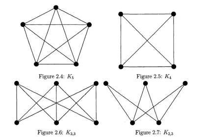
D efinition 20. A simple graph is a com plete graph if every pair of vertices
is joined by an edge. The complete graph with n vertices is denoted by K n (see Figure 2-4, 2-4) ■
Definition 21 . A 2 -v e rte x is a vertex of degree 2 and whose neighbors are ad
jacent.
Definition 22. A simple graph is bipartite if its vertices can be partitioned into
2.1 Basic Definition
Figure 2.4: K5 Figure 2.5: K±
Figure 2.6: 3 Figure 2.7: K 2,z
D efinition 23. A com plete b ipartite graph is a simple bipartite graph in which each vertex in one partite set is adjacent to all the vertices in the other partite set. I f the two partite sets have cardinalities r and s, then this graph is denoted by K rtS (see Figure 2.6, 2.7).
D efinition 24. A graph is H a m ilto n ia n if it has a spanning cycle.
D efinition 25. Two graphs G and H are hom eom orphic if both of them can be obtained from the same graph by replacing edges with paths.
D efinition 26. A p la n a r embedding of a graph is a graphical representation of the graph on the plane ( with dots representing vertices and line segment joining two dots representing edges joining the two corresponding vertices ) such that no two edges intersect except at an end-point. The edges partition the plane into regions, called faces. The edges surrounding a region is called the boundary of that region. There is exactly one face with unbound area called the e x te rio r face.
D efinition 27. A graph is p la n a r if it has a planar embedding in the plane.
D efinition 28. A graph is called o u terp la n a r if it has an embedding in the plane such that all the vertices lie on the boundary of the exterior face.
2.2 Representation of Graph
D efinition 30. An o u te r edge is an edge which lies on the boundary of the exterior face.
D efinition 31. The in n e r edge is an edge which does not lie on the boundary of the exterior face.
2.2
R ep resen tation o f Graph
2.2.1 A d ja cen cy M a trix
An a d ja cency m a tr ix of a graph G = (V, E) is an |Fj x |f/| matrix M , such that
M [i,j] = 1 if and only if vertex v-i and vertex Vj are adjacent. Adjacency matrix is the simplest way to represent graphs. However, the time and space complexity are fl(|F |2) as it requires 0 (|V |2) memory locations to store the matrix M and
0 ( |F |2) time to initiate the matrix. Figure 2.1 is an adjacency matrix for the graph in Figure 2.1.
V l V2 v3 v4 v5 Ve v7 Vs Vg Vi o V i 0 1 0 0 0 0 0 0 0 1 V2 1 0 1 0 0 0 1 0 1 0
v3 0 1 0 1 0 0 0 0 0 0
v4 0 0 1 0 1 0 1 0 0 0
V5 0 0 0 1 0 1 0 0 0 0
V& 0 0 0 0 1 0 1 0 0 0
v7 0 1 0 1 0 1 0 1 1 0
Vs 0 0 0 0 0 0 1 0 1 0 V9 0 1 0 0 0 0 1 1 0 1 VlO 1 0 0 0 0 0 0 0 1 0
Table 2.1: Adjacency matrix of the graph in Figure 2.1
2.2.2
A d ja cen cy List
An a d ja cen cy lis t of a graph G = (V,E) consists of an |Vj— element array of pointers, where the ith element points to a linked list of the vertices adjacent to the vertex without loss of generality, we shall use v, and i interchangeably.
2.3 Graph Traversing Techniques
1 — > 2 — >10
2 — > 1 — ► 3 — > 7 — > 9 3 — >2 — >4
4 — > 3 — >5 — > 7 5 — > 4 — > 6 6 — > 5 — > 7
7 — >2 — >4 — > 6 —> 8 — ► 9
8 — > 9 — > 7
9 — >2 — > 8 — >7 — >10
10 — > 1— > 9_________________________________________
Table 2.2: Adjacency lists of the graph in Figure 2.1
D efinition 32. C ro ss-p o in ter linked lists are the adjacency lists of the graph G = (V,E) such that for each vertex v in A L ist(u ),u E V , there is cross-pointer
between the vertex v in A L ist(u) and the vertex u in AList(v).
2.3
Graph Traversing Techniques
A search algorithm takes a problem as input, evaluates a number of possible so lutions, and returns a solution to the problem. The set of all possible solutions to a problem is called the search space.
Among all the search algorithms, tree search algorithm is the heart of all search techniques, and is one of the central algorithms of many game playing programs. A tree traversal is a process of visiting each vertex in a tree data structure. Such traversal can be classified by the order in which the nodes are visited. For instance, level by level (Breadth-first search), reaching a leaf vertex first before backtracking (Depth-first search), alternative-deepening search, depth-limited search, bidirec tional search and uniform-cost search.
2.3.1 D e p th F irst Search
Depth First Search (abbreviated as DFS), as its name implies, is a graph-search method that searches “deeper” when possible. Specifically, a DFS extends the current path as far as possible before backtracking to the last reached vertex and trying the next alternative path.
compo-2.3 Graph Traversing Techniques
nent and strongly connected component [48]. Later, Tarjan and Hopcroft used it to develop a linear-time algorithm for recognizing planar graph [30]. Since then, depth-first search has been used in developing optimal algorithm for a vast variety of graph-theoretic problems.
Owing to the success in using depth-first search to develop efficient graph al gorithms on the sequential computers, researchers in parallel computation had attempted to adapt the technique to parallel computers. Unfortunately, very few progresses were reported. Finally, Reif proved that depth-first search is an inher ently sequential technique [44].
It turned out that depth-first search is much more adaptable to the distributed processing setting. Chueng [9] presented the first depth-first search algorithm that runs on an asynchronous computer network. The algorithm takes 2m time and transmits 2m messages each with 0 (1) length, where m is the number of links in
the network. Awerbuch [4] improved the time bound to 4n, where n is the number of nodes in the network (note that m = 0 ( n 2)). Lakshmanan et al. [35] tightened the time bound to 2n — 2. Cidon [11] showed that the message bound can be reduced to 3m; however, Tsin [49] later showed that Cidon’s algorithm does not always perform a depth-first search over the network correctly. Tsin then corrected the flaws in Cidon’s algorithm and showed that the time and message complexity of the corrected algorithm are actually same as those of Lakshmanan et al Tsin further showed that by extending the message length from 0(1) to O(logn), the time complexity of the corrected Cidon’s algorithm can be improved to n (l + r), where 0 < r < 1. Sharma et al. [34,45] showed that one can trade message size for time and message by using messages of length 0 (n) to reduce the time and
message to 2n — 2. Makki et al. [38] improved the bounds to n (l + r), where 0 < r < 1 by using the dynamic backtracking technique. Recently, Turau [51] showed that depth-first search is also adaptable to wireless sensor network.
On the external-memory model (a model in which the input size is larger than the internal memory size), Chiang et al. [10] proposed a depth-first search algo rithm that requires 0(\n /M ]sca n (m ) + n) I/O operations, where M is the size of the internal memory, n and m are the number of vertices and the number of edges,
reposi-2.3 Graph Traversing Techniques
tory tree and used it to develop another depth-first search algorithm that requires
0 ((n + rn/B) log2(n/B ) + sort(m)) I/O operations, where B is the number of items an I/O operation can transfer from/to an external disk and sort(m) is an other primitive which is the number of I/O operations needed to sort m items striped across the external disks. The algorithm outperforms that of Chiang et al. when M = o{{n/B )/\og2(n/B )). For planar graph, Arge et al. [2] presented
a depth-first search algorithm that requires 0(sort(n) \og(n/m)) I/O operations.
The following is a brief description of depth-first search:
Initially, all the edges in the graph G — (V, E) are unexplored and all vertices are unvisited. An arbitrary vertex r is chosen as the starting point of the depth- first search. Vertex r thus becomes the current vertex of the search. In general, let v be the current vertex of the search. An unexplored edge incident on v is chosen. If the edge does not lead to an unvisited vertex, it is discarded and an other unexplored edge is chosen. This step is repeated until either an unexplored edge whose other end-point w is unvisited is encountered or vertex v runs out of unexplored edge. In the former case, the search advances to vertex w making it the current vertex. In the latter case, the search backtracks to the vertex u from which v was discovered as an unvisited vertex earlier.
A depth-first search creates a spanning tree, called dep th -first search span
ning tree (abbreviated as DFS-tree), of the given graph. The spanning tree
consists of all those edges the search uses to advance from a current vertex to an unvisited vertex. An edge in the graph is called a tree edge if it belongs to the DFS-tree and is called a back edge, otherwise. Let e = (u,v) be a tree edge. Vertex u is the p a ren t of vertex v if vertex u is visited before vertex v during the search. Vertex v is called a child of vertex u.
The depth-first search also labels each vertex v with an integer, called the
d ep th -first search num ber of v, which shall be denoted by df s(v). The inte
ger is the rank of vertex v in the ordering the vertices are visited by the depth-first search. Specifically, dfs{v) = k if vertex v is the kth unvisited vertex being turned into a current vertex by the search.
2.4 Planar Graphs and Outerplanar Graphs
A lg o rith m 1 DFS(v, u)
In p u t: The adjacency lists of G = (V, E):
{com m ent: vertex u is the parent of vertex v}
dfs(v) <— count; count <— count +1; com m ent: /* count is initialized to 1 */ for each w in the adjacency list of v do
if w is unvisited th e n D F S K v)
en d if end for
Figure 2.8: a DFS spanning tree of the graph in Figure 2.1
2.4
Planar Graphs and O uterplanar Graphs
2.4.1 P lan ar G raph
Planar graph arises naturally in real-life situation. For instance, railway maps, electric circuits are planar graphs.
Kuratowski gave the first characterization theorem for planar graphs, now known as the Kuratowski’s theorem.
T h e o rem 1. An undirected graph is planar if and only if it does not contain a subgraph that is homeomorphic to K$ or K ^ .
2.4 Planar Graphs and Outerplanar Graphs
is the number of vertices in the graph. Later, Goldstein [23] spotted an error in Auslander and Parter’s algorithm and corrected it.
The first linear-time planar graph algorithm was proposed by Hopcroft and Tarjan [31]. The algorithm is based on Auslander, Parter and Goldstein’s algo rithm. It starts from a cycle and adding to it one path at a time. Each such
new path connects two existing vertices with new edges and vertices. The process continues until either a non-planar subgraph is constructed or the entire graph is constructed. In the former case, the given graph is non-planar; in the latter case, the given graph is planar.
Lempel, Even and Cederbaum [36] used a different approach for planarity testing. Instead of starting with a cycle and adding one path at a time, they start with a single vertex and add one vertex at a time. Each time after a new vertex is added, all the previously added edges that are incident on the new vertex are connected to the vertex; new edges incident on the new vertex are then added with their other endpoints left unconnected. The process continues until a either nonplanar is constructed or the entire graph is completed. Several linear
time algorithms based on Lempel, Even and Cederbaum’s algorithm had been proposed [6,17,46].
2.4.2
O u terp lan ar G raph
An o u te rp la n a r graph is an undirected graph which can be embedded into the plane so that every vertex lies on the boundary of the exterior face. Obviously, every outerplanar graph is planar, but the converse is not true. A4 and A2)3
(Figures 2.5, 2.7) are the two smallest non-outerplanar graphs. They play a
fundamental role in characterizing outerplanar graphs.
T h e o re m 2. A graph is outerplanar if and only if it has no subgraph
homeomor-phic to K4 or A^2,3 ■
Proof. See [8].
□
T h e o rem 3. A graph is outerplanar if and only if each of its biconnected compo nents is outerplanar.
Proof. See [28].
2.5 Bucket Sort
Owing to Theorem 3, many outerpalnar graph algorithms assume that the input graph is biconnected. Brehaut [7], Mitchell [41] and Syslo et al. [47] are such examples. However, if the input graph is not biconnected, a biconnected component algorithm must be used to decompose the input graph into a collection
of biconnected components first. This could lengthen the run time of the algorithm significantly. By contrast, both Wiegers [53] and Tsin and Lin [50] do not make such assumption on the input graph.
2.5
B ucket Sort
Bucket sort is a distribution sorting method that is most suitable for sorting
d-digit integers or d-tuples of integers in which the integers are bounded by integer
k. It runs in linear time providing that k and d are small, fixed constants.
The algorithm works as follows: Let Array[0..n — 1] be an array of n d-tuples of integers in which the integers are in the range {1, 2, . . . , A;}. Then k initially empty buckets are used each of which corresponds to a distinct integer in the given range. The algorithm runs through d iterations. During the j th, 1 < j < k
iteration, a tuple Array[i] = (a^, ai2, . . . , aik) is put into bucket aik_j+1. the tuples are then combined into one list with those tuples from bucket i precede those from bucket i + 1, where 1 < i < k. The list is then used in the following iteration. A brief description of the algorithm is given below.
Algorithm 2 Bucket Sort {Array, n)
for j = 1 to k do
Bucket[i\ := 0; comment: /* initialize the Buckets */
end for
for j = 1 to ddo for i = 0 to n — 1 do
Bucket[aik_j+1] <— Bucket[aik_j+1] ® Array[i\]
{comment: Append Array[i] to Bucket aik_j+1] © is the concatenation operator}
end for
Combine the tuples in the buckets into one list such that those tuples from bucket i precede those from bucket i + 1, where 1 < i < k;
Copy the list back into A rra y[0..n — 1];
C hapter 3
A Stu d y o f M itch ell’s A lgorithm
3.1
M axim al O uterplanar A lgorithm
Mitchell’s algorithm [40] runs in linear time and space. However, it assumes that the given graph is biconnected. If the graph is not biconnected, then a biconnected component algorithm must be used to decompose the graph into a collection of biconnected subgraphs. Michell’s algorithm can then be used on each of the subgraphs to find out if any of them is not outerplanar. The given graph is outerplanar if and only if each of its biconnected components is outerplanar. Furthermore, Mitchell’s algorithm does not produce an embedding for the given graph if the graph is outerplanar.
Mitchell first presented a linear time and space algorithm for recognizing max imal outerplanar graphs. The algorithm is based on the following lemma.
T h e o rem 4. A graph G = (V, E) is maximal outerplanar if and only if either G is a triangle or
i G contains exactly 2\V\ — 3 edges, and
ii G has at least two 2-vertices, and
iii no edge of G lies on more than two triangles, and
iv for any 2-vertex u, G — u is maximal outerplanar.
Proof. See [40]. □
3.2 Outerplanar algorithm
Given a biconnected undirected graph G = (V, E). LIST is a stack used to store the 2-vertices. EDGES is the set of all the edges in the graph.
1. If |Ej ^ 2|U| — 3 then stop and report that G is not maximal outerplanar. (Based on Theorem 4(i))
2. Push all the vertices of degree 2 onto L IS T . If the size of L I S T is less than 2, then stop and report that G is not maximal outerplanar. (Based on Theorem 4(ii))
3. Repeat the following steps until a triangle is left (Based on Theorem 4(iv)):
3.1 Pop a 2-vertex N O D E from L IST ;
3.1 Find the vertices N E A R and N E X T which are adjacent to N O D E ;
3.2 Remove N O D E from the graph G;
3.3 Add (N E X T , N E A R) to P A IR S;
3 .4 If D eg(N EXT) = 2, push N E X T onto L IS T ;
If Deg(NEAR) = 2, push N E A R onto L IST ;
4. Use two-pass bucket sort to sort P A IR S and E D G E S in lexicographical order. (So that Step 5 can be done in 0 (|V |) time)
5. Compare the lists P A IR S and E D G E S. If there is an occurrence of an element in P A I R S that is not in E D G E S, then stop and report that G is not maximal outerplanar. Otherwise, report that the graph G is maximal outerplanar. (Based on Theorem 4(iii), there should be one and only one edge between the vertices adjacent to 2-vertices.)
Each time a 2—vertex is removed from L IS T S , an edge (N E X T , N E A R ) is added to P A IR S indicating that that edge must be an edge in G and hence in set E D G E S, if G is maximal outerplanar.
3.2
O uterplanar algorithm
3.3 An Example of Mitchell’s Outerplanar Algorithm
Owing to Lemma 1, Mitchell’s maximal outerplanar algorithm presented in last section can be easily modified to do outerplanar recognition. The complexity
of the resulting algorithm is still linear in the number of vertices. The modifica tion involves Steps 1 and 3 only:
Theorem 5. Let G—(V,E) be an outerplanar graph. Then \E\ < 2\V\ —3.
Proof. See [28].
□
Owing to Theorem 5, the condition “\E\ ^ 2\V\ — 3” in Step 1 is replaced by “|£ | ^ 2|Vj — 3”. Step 3 is modified as follows:
3.1 Pop a 2-vertex N O D E from LIST-,
3.2 Find the vertices N E A R and N E X T which are adjacent to N O D E;
3.3 Remove N O D E from the graph G\
3.4 Add { N E X T , N E A R) to P A IR S ;
3.5 If edge { N E X T , N E A R) does not exist in G, add it to E D G E S and add
N E A R and N E X T to each other’s adjacency list;
3.6 If Deg{NEXT) = 2, push N E X T onto LIST]
If Deg{NEAR) = 2, push N E A R onto L I S T;
Step 3.1, 3.2???, 3.4, 3 .6 require constant time. Step 3.3???, 3.5 take 0 (|R |) time.
3.3
A n E xam ple o f M itch ell’s O uterplanar A l
gorithm
3.3 An Example o f Mitchell’s Outerplanar Algorithm
EDGES
(1,2) (1,6)
(2.3) (3.4) (4.5) (5.6)
(2.6)
LIST 5 4 3 1 PAIRS
Figure 3.1: An Illustration of Mitchell’s Algorithm
3.3.1
R em oval o f 2-vertices
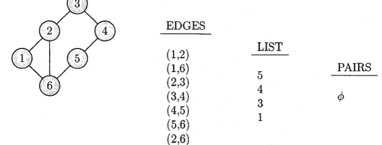
The algorithm first checks if the condition \E\ < 2\V\ — 3 holds. Since the con dition holds, all the vertices of degree 2 are pushed onto the stack L I S T (see Figure 3.1). As the size of L I S T is greater than 2, the algorithm begins to pop the stack L I S T S .
The first vertex popped out is the vertex 5 (see Figure 3.2). Since vertices 4 and 6 are adjacent to 5, the edge (4,6) is added to P A IR S . Since the edge (4,6) does not exist in the graph, it is added to ED G E S.
Deg{4) and Deg(6) remain unchanged.
LIST 4 3 1 PAIRS (4,6) EDGES (4.6)
(1,2)
( 1.6) (2.3) (3.4) (4.5) (5.6) (2 .6)
Figure 3.2: An Illustration of Mitchell’s Algorithm: after removal of node 5
The removal of node 4 is similar with node 5. The updated graph, L I S T , E D G E S and P A I R S are shown in Figure 3.3.
pre-3.3 An Example of Mitchell’s Outerplanar Algorithm
EDGES
(6.3) (4.6)
(1,2)
(1.6)
(2.3) (3.4) (4.5) (5.6)
(2.6)
Figure 3.3: An Illustration of Mitchell’s Algorithm: after removal of node 4 LIST
3 1
PAIRS
(6,3) (4,6)
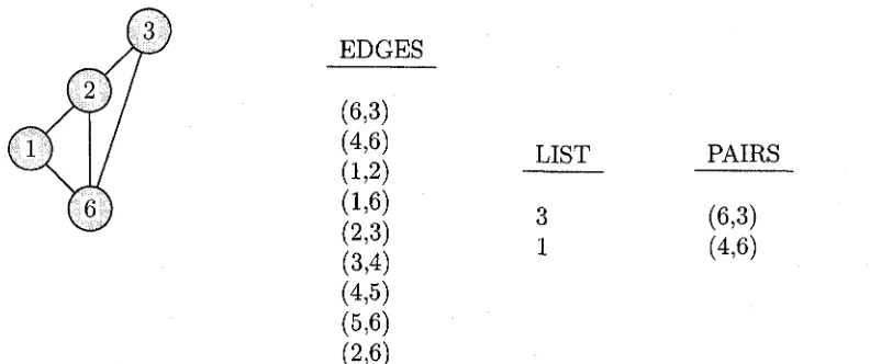
vious step is that (2,6) already exists in the graph, so there is no need to add it into E D G E S . Since Deg(2) and Deg{6) have changed to 2, there are thus pushed onto the L IS T .
EDGES
(6.3)
(4.6) LIST PAIRS
(1,2)
(1.6) 6 (2,6)
(2.3) 2 (6,3)
(3.4) 1 (4,6)
(4.5) (5.6)
(2 .6 )
Figure 3.4: An Illustration of Mitchell’s Algorithm: after removal of node 3
Figure 3.5 shows the graph after the last removal of vertex from L I S T is per formed. If the given graph is outerplanar, it would always appear like this: a single edge connect two vertices which are stored at the bottom of L IS T .
3.3 An Example of Mitchell’s Outerplanar Algorithm
EDGES
(6.3) (4.6)
(1,2)
( 1.6)
(2.3) (3.4) (4.5) (5.6)
( 2 .6 )
LIST
PAIRS
2
1
(1,2) (2,6)
(6,3) (4,6)
Figure 3.5: An Illustration of Mitchell’s Algorithm: after removal of node 6
Figure 3.6: An Illustration of Mitchell’s Algorithm: P A I R S and E D G E S after all the 2—vertices are removed
3.3.2
B u ck et Sort
Both the lists E D G E S and P A I R S can be sorted by a two-pass Bucket Sort. Each pair in E D G E S and P A I R S consists of two integers from 1 to 6. Before sorting, every pair is adjusted so that the first integer is no greater than the second integer.
The arrays in Figure 3.7 are then sorted using 2-pass Bucket sort. The buckets are labeled from 1 to 6. In the first pass, each pair in P A I R S (ED G E S, respec tively) is put into a bucket whose label is identical to the second integer of the ordered pair. A partially sorted P A I R S (ED G E S, respectively) (sorted by their second integer) is obtained. In the second pass, each pair in P A I R S (ED GES,
respectively) is put into a bucket whose label is identical to the first integer of the ordered pair. A sorted P A I R S (EDG ES, respectively) is then obtained.
Fig-EDGES
(2,1)
(6.3) (4.6)
(1,2)
(1.6)
(2.3) (3.4) (4.5) (5.6)
(2 .6 )
PAIRS
(1,2) (2,6)
3.3 An Example of Mitchell’s Outerplanar Algorithm
EDGES
PAIRS
(3,6)
---(1,2) (1,2)
(3,6)
(1 2) (1'2)
6 ( 2 '6 >
2 3 W
( M ) (4 ’6)
(4.5) (5.6)
(2.6)
Figure 3.7: An Illustration of Mitchell’s Algorithm: P A I R S and E D G E S before Bucket Sort
ures 3.8 and 3.9 show the results of Bucket sort.
EDGES
(1.2)
(34) f1'2)
4 5 <2'6>
<*•>
(4.6) l4,bj
(1.6)
(5.6)
(2 .6 )
Figure 3.8: An Illustration of Mitchell’s Algorithm: P A I R S and E D G E S after one-pass Bucket Sort
3.3.3
C heck P A IR S and E D G E S
3.4 Implementation
EDGES
(1,2)
(1,2) (1,2)
(1,6)
(2.3)
(2,6)
(3.4) (3,6) (4.5) (4.6) (5.6)
PAIRS
(1,2) (2,6)
(3.6) (4.6)
Figure 3.9: An Illustration of Mitchell’s Algorithm: P A I R S and E D G E S after a two-pass Bucket Sort
3.4
Im p lem en tation
Unfortunately, the presentation of Mitchell’s outerplanar algorithm in Mitchell’s original paper [41] is very brief. It is not at all clear that the algorithm can be implemented in linear time and space. For instance, in Step 3.5, the algorithm has to check whether the edge (N E A R , N E X T ) already exists in the graph G before it is added to E D G E S. This could be accomplished by scanning the adjacency list of N E X T for the vertex N E A R . The vertex N E A R appears in the adjacency list if and only if the edge (N E A R , N E X T ) exists in G. Since it takes 0(\V\)
time to search an adjacency list in the worst case, if there are 0 (|I/|) N E X T s ,
the algorithm would take 0 (|U |2) time rather than linear time.
3.4.1
Our stra teg ie s in th e im p lem en ta tio n
We adopt the following strategies in implementing Mitchell’s algorithm:
• The adjacency list data structure is used to represent the input graph G =
• Delay checking if the edge (N E X T , N E A R ) exists in the given graph until either N E X T or N E A R is popped out of L I S T (i.e. D e g (N E X T ) = 2 or
D eg(NE AR ) = 2).
• In order to save the time on scanning the adjacency list, we shorten the adjacency list by deleting all the nodes of degree 0 . As we often deal with
3.4 Implementation
node with degree 2, it takes only 0 (1) to scan this adjacency list.
3.4.2
M ain S te p s o f our Im p lem en ta tio n
We briefly describe the main steps of our implementation first.
1. Check whether |E\ < 2\V\ — 3 . If not, then Stop.
2. Push all the vertices with degree 2 onto L I S T . If size(L IST ) < 2, then Stop.
3. Pop N O D E from L I S T; Find the vertices N E A R and N E X T which are adjacent to NODE; Add ( N E X T , N E A R ) to P A IR S; Remove N O D E
from the graph.
4. Add N E A R and N E X T , each with a mark, to each other’s adjacency list.
5. If Deg(NEXT) = 2, check if any node with a mark in the adjacency list is a duplicate entry, if it is, then delete the node with a mark; otherwise add the node to adjacency list of N E X T and update D eg (N E X T ) accordingly. Do the same for vertex N E A R if Deg(NEAR) = 2.
6. If Deg(NEXT) = 2 or Deg(NEAR) = 2, push it onto L IS T .
7. Use a two-pass Bucket Sort on PAIRS and EDGES.
8. If there is an occurrence of an element in P A I R S that is not in E D G E S,
then Stop, else report that the given graph G is outerplanar.
The changes take place in Step 4 and 5. To save the efficiency, our algorithm does not check whether the edge (NEAR,NEXT) exists in adjacency list until
Deg(NEXT) or Deg(NEAR) = 2. In this way, it takes only 0(2) times in stead of 0(|Wj) in Mitchell’s algorithm.
3.4 Implementation
3.4 .3
A D eta ile d Im p lem en ta tio n
3.4 Implementation
Algorithm 3 An Implementation of Mitchell’s Outerplanar Algorithm
1. if ( |£ | < 2\V\ - 3) th e n
2. Output ” No” 3. en d if;
4. L I S T <- {v\Deg[v) = 2}; P A I R S <- 0; 5. if (\LIST\ < 2) th e n
6. Output ”No” 7. en d if;
8. for L = 1 to |Vj — 2 do
9. N O D E <- p o p (LIST)]
N E A R , N E X T <— the two vertices adjacent to N O D E;
10. Add (N E A R , N E X T) to list P A I R S;
11. Remove N O D E from the graph;
12. Decrement Deg(NEAR) and D eg(NEXT)]
13. if (D eg (N E A R) < 2) th e n 14. ChkAdj (N E A R , NEXT)-,
15. en d if
16. if (D eg (N E X T ) < 2) th e n 17. ChkAdj ( N E X T , N E A R); 18. e n d if;
19. if (Deg(NEAR) > 2) A (D eg(N E X T ) > 2) th e n
20. AddRed(NEXT, NEAR)]
21. e n d if
22. if (Deg(NEAR) < 2) th e n Add N E A R to LIST]
23. if (D eg (N E X T ) < 2) th e n Add N E X T to LIST]
24. if (\LIST\ - L < 2) th e n 25. Output ”No”
26. en d if 27. en d for;
28. Add the edge (N E A R , N E X T ) to EDGES]
29. Lexicographically sort EDGES]
30. Lexicographically sort P A IRS]
31. if there is an edge in P A I R S and not in E D G E S th e n 32. Output ”No”
33. else
3.4 Implementation
Algorithm 4 Check the adjacency list of vertex a for vertex b
Procedure ChkAdj(a,b)
if (there is no b colored white in the adjacency list of a) then
AddWhite(a,6);
end if ;
for (each vertex v in the adjacency list of a) do if (Deg[v] = 0) then Remove v from the list;
else if (v is red) then
if (^ another v colored white in the list) then
RemoveRed((a, v))-, AddWhite(a, v);
else RemoveRed(a,v);
A lgorithm 5 Add White Node
Procedure AddWhite(a,b)
Add the edge (a,6) to list E D G E S
Add a and b with color white to the end of each other’s adjacency list Increment(Deg(a)); Increment(Deg(b))
In Step 1, if \E\ > 2\V\ — 3, then by Theorem 5, the input graph cannot be outerplanar. The algorithm thus terminates its execution and outputs a ”No” .
In Step 4, the set of vertices of degree 2 are pushed onto the stack L IS T . The list of edges P A I R S is initialized to the empty set.
In Step 9, a vertex N O D E is popped out of the stack L IS T . Since N O D E
is of degree 2, it can have only two adjacent vertices, N E A R and N E X T .
In Step 10, the edge ( N E X T , N E A R ) is added to P A IR S .
In Step 11, vertex N O D E is removed from the graph by setting Deg(NODE)
to 0.
In Step 12, the degrees of D eg (N E X T ) and Deg(NEAR) are incremented according.
In Steps 1 3 -1 5 , if the D eg(NEAR) < 2, then its adjacency list is scanned for
N E X T . The existence of a N E X T vertex colored white indicates that the edge
3.4 Implementation
A lg o rith m 6 Add Red Node__________________________ P ro c e d u re AddRed(a,b)
Add b with color red to the beginning of g’s adjacency list
A lg o rith m 7 Remove Red Node P ro c e d u re RemoveRed(a,b)
Remove b (colored red) from the adjacency list of a
of N E A R (N E X t, respectively). This effectively adds the edge (N E A R , N E X T )
to G. Therefore, the edge (N E A R , N E X T ) is also added to E D G E S and the de grees of a and b are incremented accordingly. Next, the adjacency list of N E A R
is scanned. For each vertex v in the list, if Deg(v) = 0, vertex v is removed rom the list. If v is colored red and there is a vertex v colored white in the list, then the red v is removed; otherwise, the red v is removed, and a white v is added to the adjacency of N E A R while a white N E A R is added to the adjacency list of v. Moreover, the edge (N E A R ,v ) is added to E D G E S and Deg(v) and
Deg (N E A R ) are incremented accordingly.
Steps 16-18 are similar to Steps 13-15.
Steps 19 — 21, if neither D eg(NEAR) < 2 nor D eg (N E X T ) < 2, then a vertex N E X T (N E A R , respectively) colored red is added to the adjacency list
of N E A R ( N E X T , respectively). When D eg(NEAR) (D eg(N E X T ), respec tively) finally becomes two or less, the red N E X T (N E A R , respectively) will be processed in Steps 13-15 (16-19, respectively).
In Steps 22 and 23, vertex N E A R ( N E X T , respectively) is pushed onto the stack L I S T if D eg(NEAR) < 2, (D eg(N E X T ) < 2, respectively)
In Steps 24 — 26, If there are less then two vertices on the stack L I S T and fewer than | V| — 2 vertices had been popped out of L I T S , then execution of the algorithm terminates and the graph G is reported as non-outerplanar.
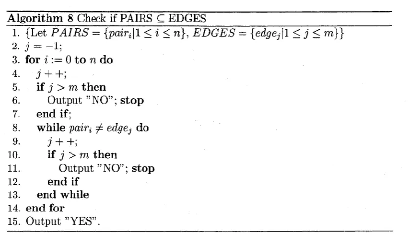
In Steps 29-35, both E D G E S and P A I R S are sorted lexicographically using bucket sort. This is to ensured that checking if P A I R S C E D G E S can be carried
3.4 Implementation
A lg o rith m 8 Check if PAIRS C EDGES________________________
1. {Let P A I R S = {pairi\l < i < n } , E D G E S = {edgej\l < j < m}}
2- j = - 1;
3. for % := 0 to n do 4- j + +;
5. if j > m th e n
6. Output ”NO” ; sto p 7. en d if;
8. w hile pairi ^ edgej do 9. j + +;
10. if j > m th e n
11. Output ”NO” ; sto p
12. en d if 13. en d w hile 14. en d for
15. Output ”YES” .
3.4 .4
A n Illu stra tio n o f M itc h e ll’s O u terplanar A lg o rith m
We use the example in Figure 3.10 to illustrate Mitchell’s algorithm for outerpla- narity testing. After reading the input graph file, the Adjacency Lists and the elements in E D G E S would be as shown in Figure 3.10. The algorithm starts with verifying |£j < 2\V\ — 3. Since \V\ = 6 and \E\ = 7, the condition is satisfied. The next step is to push all vertices that are of degree 2 onto L I S T and initialize
P A I R S to 0.
EDGES
(1,2)
(1,6)
(2.3) (3.4) (4.5) (5.6)
(2.6)
Adjacency List
1 : 2 6 2 : 1 6 3 3 : 2 4 4 : 3 5 5 : 4 6 6 : 1 2 5
LIST 5 4 3 1 PAIRS
Figure 3.10: An Illustration of Mitchell’s Outerplaner Algorithm; |Vj = 6.
Node 5 is the first vertex popped out of L I S T and removed from G. Since the two vertices adjacent to vertex 5 are vertices 4 and 6. the edge (4,6) is added to
3.4 Implementation
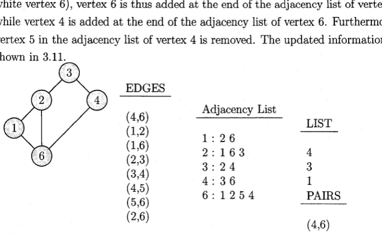
white vertex 6), vertex 6 is thus added at the end of the adjacency list of vertex 4
while vertex 4 is added at the end of the adjacency list of vertex 6. Furthermore, vertex 5 in the adjacency list of vertex 4 is removed. The updated information is shown in 3.11.
EDGES
(4.6)
(1,2)
(1.6)
(2.3) (3.4) (4.5) (5.6)
(2 .6)
Adjacency List
1 : 2 6 2 : 1 6 3 3 : 2 4 4 : 3 6
6 : 1 2 5 4
LIST 4 3 1 PAIRS (4,6)
Figure 3.11: An Illustration of Mitchell’s Algorithm: After removal of vertex 5
The removal of vertex 4 is similar to vertex 5 (see Figure 3.12).
EDGES
(3.6) (4.6)
(1,2)
(1.6)
(2.3) (3.4) (4.5) (5.6)
( 2 .6 )
Adjacency List
LIST
1 : 2 6
2 : 1 6 3 3
3 : 2 6 1
6 : 1 2 5 4 3 PAIRS
(3.6) (4.6)
Figure 3.12: An Illustration of Mitchell’s Algorithm: After removal of vertex 4
3.4 Implementation
EDGES
(3,6)
(4,6) Adjacency List LIST (1,2)
(1,6) 1 : 2 6 6
(2,3) 2 : 1 6 2
(3,4) 6 : 1 2 1
(4,5) PAIRS
(5,6)
(2,6) (2,6)
(3.6) (4.6)
Figure 3.13: An Illustration of Mitchell’s Algorithm: After removal of vertex 3
The next vertex popped out of L I S T is 6. The edge (1,2) is then added to
P A I R S . Since Deg( 1) < 2, the adjacency list of vertex 1 is scanned and vertex
6 is removed from the list. Furthermore, as there is an unmarked vertex 2 in the
list, no edge (1,2) is added to ED G ES. Similarly, as Deg(2) < 2, the adjacency list of vertex 2 is scanned and vertex 6 is removed from the list. Finally an edge
(1,2) is added to ED G E S.
Finally, as P A I R S C E D G E S , the algorithm thus terminates execution with
a ” Yes” .
EDGES
(1,2)
(3.6)
(4.6) Adjacency List LIST
(1,2)
(1.6) 1 : 2 2
(2.3) 2 : 1 1
(3.4) PAIRS
(4.5)
(5.6) (1,2)
(2.6) (2,6)
(3.6) (4.6)
C hapter 4
A S tu d y o f W ieg ers’ A lgorithm
4.1
O uterplanar algorithm
In contrast with Mitchell’s algorithm, Wiegers’ Outerplanar algorithm [53] ac cepts non-biconnected graphs as the input graph and performs no sorting. This algorithm uses a 2—reducible graph testing and an edge-coloring technique. Sim ilar to Mitchell’s algorithm, Wiegers’ algorithm repeatedly removes vertices of degree two or less from the graph; whenever a vertex of degree two is removed, a new edge joining its two neighbors is added to the graph if the edge does not exist. If the algorithm runs out of vertices of degree two or less before reducing the input graph into an edgeless graph, the algorithm terminates its execution and reports that the graph is non-outerplanar. This is because the graph must contain a subgraph that is homeomorphic to K4. The edge-coloring technique is used to keep track of the number of triangles each edge belongs to. If any edge belongs to more than two triangles, the algorithm would report that the graph is non-outerplanar indicating that the graph contains a subgraph that is homeo morphic to A2)3.
4.1.1
T h e 2-R ed u cib le G raph A lgorith m
D efinition 33. [53] A graph G=(V,E) is 2—reducible if and only if
E = 0, or
3u € V such that Deg(u) < 1, Gu = G — {«} is 2-reducible, or