ABSTRACT
WANG, ZHAO. Efficient Linear Matrix Solver and Its Hardware Implementations Dedicated to Faster-Than-Real-Time Dynamic Simulation of Large Scale of Power System. (Under the direction of Dr. Paul Franzon).
Dynamic simulation is a crucial aspect in power system modeling. The transient instability phenomena can develop quickly and lead to the collapse of a power system. However, the tran-sient stability forecast is challenging both mathematically and physically - it involves repetitive solutions to a high-dimension linear system equation in short simulation time intervals, which can be difficult to reach faster-than-real-time anticipation. Thus, it is essential to establish a high-speed simulator for online assessment of the actual power systems.
In this dissertation, I begin with the review of the power system mathematical model and the dynamic simulation flow, and then I focus on how to solve the system equations and differential equations efficiently. I thoroughly reviewed the state-of-the-art dynamic simulation method-ologies. To perform dynamic simulation, researchers have explored feasibilities on varieties of methodologies.
By reviewing state-of-the-art power system dynamic simulation, we can see the insufficient capabilities of the existing simulators. Given the large system size and the stringent real-time requirement, solving the linear equation will be time-consuming. Thus, novel breakthroughs in the algorithm and computational devices are needed to accelerate the simulation.
To solve the problem, I used prior research in the field as a foundation. Hence, I analyzed the scalability of the mixed-signal approach developed by the researches in Ecole polytechnique federale de Lausanne (EPFL). While I discovered that this approach is successful when sim-ulating 100-bus systems, it was challenging to implement on systems with 10,000-bus scales. Given the scalability of analog devices and signal propagation delay, we decided to focus on numerical solutions.
I noticed the change to the admittance matrix is mathematically low-rank upon the fault. Therefore, we can take advantage of the low-rank properties when handling the network equa-tion. A preconditioned Richardson iterative method is hence proposed. After that, the spar-sification strategy to the preconditioning matrix is proposed to trade-off the convergence and the computational complexity. In this case, most of the arithmetics are converted into the sparse matrix-vector multiplications (SpMVs) and implemented on the Graphics Processing Unit (GPU). It can successfully simulate IEEE benchmarks, with the largest scale of 9,241 buses. However, the simulation was not efficient while simulating over 20,000-bus Western Elec-tricity Coordinating Council(WECC) benchmarks.
and the Sherman-Morrison-Woodbury formula. Low-rank property is still taken advantage of. Meanwhile, the matrix dimension is lowered, as we only need to track the state variables of the generators. For better parallel ability, the common L-U methodology is replaced with the matrix-vector multiplication (MVM) to solve the linear system Ax = b. A detailed generator model is also implemented together with the classical generator model. Two NVIDIA GPUs are used for implementation: GeForce GTX 960 (GTX960) and Tesla K40c (K40c), and approximately 4∼5 faster than real-time performance is achieved upon 2,000 generator-buses system, which can contain 20,000 to 50,000 buses. Scalability is also explored on larger systems. Meanwhile, I further explored the performance enhancement with more advanced GPUs or multi-GPU architecture. In addition to the one-line cut-off scenario, multi-line change scenarios are also evaluated. Some preliminary experimental results indicated that the manipulation on higher rank matrix change remains efficient.
©Copyright 2018 by Zhao Wang
Efficient Linear Matrix Solver and Its Hardware Implementations Dedicated to Faster-Than-Real-Time Dynamic Simulation of Large Scale of Power System
by Zhao Wang
A dissertation submitted to the Graduate Faculty of North Carolina State University
in partial fulfillment of the requirements for the Degree of
Doctor of Philosophy
Computer Engineering
Raleigh, North Carolina
2018
APPROVED BY:
Dr. William Davis Dr. Carl Kelley
Dr. James Tuck Dr. Paul Franzon
DEDICATION
BIOGRAPHY
ACKNOWLEDGEMENTS
Foremost, I would like to thank my advisor, Dr. Paul D Franzon, for his help, encouragement, and patience throughout my graduate study. I’m lucky to be part of his research group, which covers a wide variety of research areas and a vast of interesting cutting-edge researches. He is always helpful, supportive and encouraging during my research, and I never felt alone in my research journey. His optimism and his energetic attitudes towards his life and his students will always be with me even I leave NCSU.
I’m very grateful to Professor Rhett Davis, who has been instructor of my teaching-assistant courses for many semesters, for his support, encouragements and considerations in many oc-casions. His positive attitudes and kindness personalities will always influence me. I’m also grateful to Professors James Tuck, Huiyang Zhou and Tim Kelley for their valuable and even vital advising and feedback on my work. I would also like to show my thanks to Dr. Steve Lipa for his knowledgeable and patient discussion and feedback. My sincere thanks also go to Pro-fessors Aranya Chakrabortty, Ning Lu, as well as students Yao Meng and Nan Xue for advising me on the power system fields that I’m not familiar with. I would also like to express my thank to Dr. Chao Li, NCSU alumni graduated in 2016, for all his technical advising and discussion on GPU architecture and CUDA programming at the beginning of my research.
The research project is funded by ABB. I would gratefully acknowledge Dr. Alexandre Oudalov and other related representatives in ABB, as well as the University of EPFL researchers for sharing their research results. Throughout the discussions and feedback from Dr. Xiaoming Feng in ABB, I learned quite a lot, and enjoyed all the happiness and struggles in the past three and half years. Thank you for your time and patience on my work.
I had the pleasure with all my brilliant fellow group members with the friendship and inter-esting discussions on various topics. I was fortune to intern at IBM and Synopsys, throughout the experiences my professional skills get improved a lot. I would also thank to all my team-mates in our Chinese students soccer team with the pleasant leisure time and unforgettable moments we shared during my Ph.D. life.
TABLE OF CONTENTS
LIST OF TABLES . . . vii
LIST OF FIGURES . . . .viii
Chapter 1 Introduction . . . 1
Chapter 2 Background and Related Works. . . 6
2.1 Introduction . . . 6
2.2 Background . . . 7
2.2.1 Dynamic Simulation Mathematics . . . 7
2.2.2 Simulation Process . . . 16
2.3 Real Time Challenges . . . 18
2.4 Prior Work . . . 18
2.4.1 Analog Approaches . . . 19
2.4.2 Digital Approaches . . . 19
2.5 GPU Architectures and CUDA Programming . . . 20
Chapter 3 A Feasibility Evaluation on Analog Approach . . . 30
3.1 Introduction . . . 30
3.2 Numerical Assumptions on Transmission Lines . . . 32
3.3 Chip Scales of FPPNS . . . 33
3.3.1 ADCs and DACs . . . 33
3.3.2 Reconfigurable Resistor Network . . . 33
3.3.3 Calibration . . . 37
3.3.4 Packaging . . . 38
3.4 Conclusions . . . 39
Chapter 4 A Preliminary Numerical Approach Based on the Preconditioned Richardson Iterative Method . . . 40
4.1 Introduction . . . 40
4.2 Convergence Analysis of Stationary Iterative Methods . . . 41
4.3 Preconditioned Richardson Iterative Approach on Handling One-line Fault . . . . 42
4.3.1 Preconditioner Design: Approximation of the Inverse . . . 43
4.3.2 Sparsification of the Preconditioner . . . 51
4.4 SpMV on GPU . . . 56
4.5 Hardware Implementations and Its Optimizations . . . 60
4.5.1 Hardware Implementations . . . 60
4.5.2 Optimizations . . . 61
4.6 Experimental Results . . . 66
4.6.1 Preconditioner Verification . . . 66
4.6.2 Hardware Implementation Results . . . 68
4.6.3 Optimization Efforts . . . 70
Chapter 5 Efficient Faster-than-real-time Dynamic Simulator Based on Block
Gauss Elimination and Sherman-Morrison-Woodbury Formula . . . 75
5.1 Introduction . . . 75
5.2 Mathematics related to Block Gauss Elimination and Sherman-Morrison-Woodbury Formula . . . 76
5.3 Hardware and Software Implementations . . . 80
5.3.1 Fault Handling Process . . . 80
5.3.2 MVM on GPU in Modified Euler’s Method . . . 84
5.3.3 Generator Differential Equations in Modified Euler’s Method . . . 89
5.4 Experimental Results . . . 93
5.4.1 Performance Demonstration . . . 93
5.4.2 Waveform Verification . . . 95
5.4.3 Performance Analysis . . . 101
5.4.4 Real-time Consistency . . . 104
5.4.5 Forecasting . . . 108
5.5 Future Work . . . 110
5.5.1 Performance Improvements on One-line Fault Scenario . . . 110
5.5.2 Better Simulation Accuracy . . . 114
5.5.3 Performance Analysis of rank-k Correction Scenario . . . 116
5.6 Conclusions . . . 118
Chapter 6 Conclusion . . . .121
References. . . .123
Appendices . . . .130
Appendix A Proof of Reduced Matrix Rank-1 Correction . . . 131
A.1 Problem Statement . . . 131
A.2 Proposition . . . 132
A.3 Proof . . . 132
Appendix B Proof of Reduced Matrix Rank-p Correction . . . 136
B.1 Proposition . . . 136
LIST OF TABLES
Table 3.1 Percentage of Nets That Do Not Meet the Assumption That Permits
Separa-tion of Real and Imaginary Networks . . . 32
Table 4.1 Corresponding M for different iterative methods . . . 42
Table 4.2 Convergence by Different Iterative Method for case1354pegase . . . 42
Table 4.3 Average Nonzeros per Row of ˆP0 . . . 66
Table 4.4 Statistics of Fault Convergences upon case1354pegase, withρ(M0) = 0.243 . . 67
Table 4.5 Statistics of Spectral Clustering . . . 71
Table 5.1 Comparison of Major Specs of Different GPUs . . . 94
Table 5.2 Time Distributions for 21,671-bus WECC system (i)classical model (ii)detailed model . . . 94
Table 5.3 Proportion of Time Distributions for 21,671-bus WECC system (i)classical model (ii)detailed model . . . 94
Table 5.4 Time Distributions for 54,815-bus WECC system (i)classical model (ii)detailed model . . . 95
Table 5.5 Proportion of Time Distributions for 54,815-bus WECC system (i)classical model (ii)detailed model . . . 95
Table 5.6 Timing Ratios of K40c to GTX960 on two WECC test systems (i)classical model of 21,671-bus WECC system (ii)classical model of 54,815-bus WECC system (iii)detailed model of 21,671-54,815-bus WECC system (iv)detailed model of 54,815-bus WECC system . . . 103
Table 5.7 Timing Statistics of GTX960 on 21,671-bus WECC System with Detailed Generator Model(s) . . . 105
Table 5.8 Timing Statistics of K40c on 21,671-bus WECC System with Detailed Gen-erator Model(s) . . . 105
Table 5.9 Timing Statistics of 10,000 Times of 4,000 consecutive MVMs on K40c . . . . 108
Table 5.10 Major Specifications of NVIDIA Tesla K20c GPU(K20c), in Comparison with K40c . . . 111
LIST OF FIGURES
Figure 1.1 Schematical Illustration of Continental European Transmission Network . . . 5
Figure 2.1 Flow Chart of a Generator and Its Controller Module, Together with the Admittance Network for Dynamic Simulation . . . 8
Figure 2.2 Machine Model GENSAL . . . 10
Figure 2.3 Exciter ESST1A and ESST1A GE . . . 11
Figure 2.4 Governor WSIEG1 . . . 12
Figure 2.5 Stabilizer PSS2A . . . 13
Figure 2.6 Distribution of Node’s Degrees in case9241pegase . . . 15
Figure 2.7 Cummulative Distribution Function of the Magnitude of Transmission Lines’ Impedances(Zoomed In) . . . 16
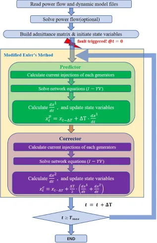
Figure 2.8 Simulation Flow Chart . . . 17
Figure 2.9 Architecture of NVIDIA K40 GPU . . . 21
Figure 2.10 Zoom-In of Each SMX in K40 . . . 22
Figure 2.11 Quad Warp Scheduler in K40 . . . 23
Figure 2.12 Comparison of GPU and CPU Architectures [54] . . . 24
Figure 2.13 The Compilation Process for NVCC . . . 26
Figure 2.14 Processing Flow on CUDA [8] . . . 27
Figure 2.15 Illustration of Grid, Thread Block and Threads . . . 28
Figure 3.1 Architecture of the EPFL Mixed-signal Emulator System [21] . . . 31
Figure 3.2 EPFL Mixed-Signal Emulator Network Details [21] . . . 34
Figure 3.3 On-chip Programmable Resistor . . . 35
Figure 3.4 MOSFET Resistors . . . 37
Figure 3.5 Overall Concept for Resistor Array . . . 39
Figure 4.1 Classification of Solvers for Linear Systems . . . 41
Figure 4.2 Example of Mini-Social-Network Matrix Reordering . . . 44
Figure 4.3 Distribution ofρdin case1354pegase Test Case . . . 55
Figure 4.4 Pros and Cons Among Different Sparse Matrix Formats [57] . . . 57
Figure 4.5 The workflow of auto-tuning framework . . . 59
Figure 4.6 SMAT Architecture . . . 59
Figure 4.7 Comparison Between Naive C Implementation and Parallel Implementation via OpenMP . . . 60
Figure 4.8 Comparison of the Sparsified Preconditioner Outlook Before and After Being Clustered . . . 63
Figure 4.9 SpMV Data Traffic Before Matrix Being Clustered . . . 63
Figure 4.10 SpMV Data Traffic After Matrix Being Clustered . . . 64
Figure 4.11 Performance Comparison Among Different Architectures and Different Im-plementations . . . 69
Figure 4.12 Matrix to Reflect Numbers of Nonzeros in ˆP0 Among Clusters . . . 72
Figure 5.1 Instantly Obtained Items due to Symmetricity . . . 81
Figure 5.2 Fault Handling Process in Details . . . 82
Figure 5.3 Directory Hierarchy ofYmm−10 . . . 84
Figure 5.4 3×3 Matrix Example of L-U Method . . . 85
Figure 5.5 Schematic of Two Phases of MVM . . . 87
Figure 5.6 Schematic ofAx=y MVM Example on GPU withm×pExample [7] . . . . 88
Figure 5.7 Computation Time Demonstration Between L-U Method and Matrix-Vector Multiplication on GTX960 . . . 88
Figure 5.8 Current Flow of the Generator-Bus with Multiple Generators . . . 90
Figure 5.9 Generators with Different Models on the Same Bus . . . 90
Figure 5.10 Data and Index Interactions Among Network, Generator and Generator Model Type Kernels . . . 92
Figure 5.11 Bus-30 Waveform Comparison Among our implementation, the GridPACKT M, and the Matlab Theoretical Result on 39-bus IEEE System, Classical Gen-erator Model Used . . . 96
Figure 5.12 Configurations of the GridPACKT M 3.1 Simulation on IEEE-145 Detailed Model . . . 97
Figure 5.13 Simulation Failure Using the GridPACKT M 3.1 on IEEE-145 Detailed Model 98 Figure 5.14 Simulation Intermediate Data Dumped Out Using the GridPACKT M 3.1 on IEEE-145 Detailed Model . . . 99
Figure 5.15 Dump-outs of Generator Dynamic State Variables for IEEE-145 Detailed Model Simulated on K40c . . . 100
Figure 5.16 2.5s Post-fault IEEE-145 Detailed Model Simulation Performance on K40 . . 100
Figure 5.17 10s Post-fault IEEE-145 Detailed Model Simulation Performance on K40 . . 101
Figure 5.18 Histogram by Performing 10,000 Times Dynamic Simulation with Random Fault of WECC 21,671-bus System with Detailed Generator Model on GTX960106 Figure 5.19 Histogram by Performing 10,000 Times Dynamic Simulation with Random Fault of WECC 21,671-bus System with Detailed Generator Model on K40c . 107 Figure 5.20 Histogram by Performing 10,000 Times of 4,000 consecutive MVMs on K40c 108 Figure 5.21 Matrix-Vector Multiplication Computation Time on NVIDIA GeForce GTX960 GPU . . . 109
Figure 5.22 Faster Than Real Time Prediction in Natural Logarithm on NVIDIA Tesla GTX960 GPU . . . 110
Figure 5.23 Single-Precision General Matrix-Vector Multiplication(SGEMV) Computa-tion Time on NVIDIA Titan X Pascal GPU(TitanX) [48] . . . 111
Figure 5.24 Single-Precision Complex General Matrix-Vector Multiplication(CGEMV) Computation Time on Multiple NVIDIA K20c GPUs(K20c) [1] . . . 112
Figure 5.25 Comparison on Single-Precision General MVM(SGEMV) and Symmetrical General MVM(SSYMV) Computation Times on Single K20c [1] . . . 114
Figure 5.26 Comparison on Single-Precision Complex General MVM(CGEMV) and Her-mitian MVM(CHEMV) Computation Times on Single K20c [1] . . . 115
Chapter 1
Introduction
New requirements for power systems are needed and the development of power grids leading to a smart grid is in progress. Today, because the power consumption is steadily increasing, power grids are running closer and closer to their operating limits. On the other hand, large power system frequency/voltage fluctuations due to severe faults in trunk transmission lines or major generating units may trip-off other facilities and result in large-scale power system blackouts. To prevent such blackouts, development of an accurate and fast power system dynamic simulation tool is required [32]. There is a fundamental need to establish a very high-speed power system simulator for online security assessment, to foresee what is happening during a time after a fault occurs in the system. Such a simulator could be combined with economic and ecologic aspects to guarantee ideal and instantaneous decision making [23].
power system real time simulation.
Since the 1960s, extensive and ever continuing research has been conducted to overcome the speed bottleneck of numerical simulators using parallel computing hardware [45]. Currently, modern massive parallel hardware architectures such as multi-core/many-core processors, com-putation platforms on GPUs or Field Programmable Gate Arrays (FPGA) are used to overcome the computational difficulties. However, the excessively high volume of arithmetic complexity, as well as the lack of parallelization makes it difficult to achieve any breakthroughs.
In contrast to the numerical simulators, researchers in this field have also tried analog approaches to meet real-time demands. The rationale behind the analog simulators is to avoid the heavy matrix arithmetics of the grid. The analog Kirchhoff grid is used to connect the generator model equation solvers, and load model solvers through the grid. However, there are several severe significant limitations. First, when the scale of grid is large, the chip will require a massive number of passive devices, which makes the whole simulator bulk in size. Moreover, when the scale increases, the number of nodes will also increase. Since we need to measure the nodal voltages, we need to get the superimposition of all the current source signals to the nodes to be measured. As a result, it is likely that some signal source will propagate through a long path to its far-end node, making the propagation delay longer than expected, referred as the Elmore delay model [14]. To make it worse, due to the large simulator size, the interconnections between the circuit boards will also increase the timing budget. In [23], researchers in EPFL have expended great efforts on mixed-signal emulators with necessary numerical approximations to speed up the emulation, which can support the emulation of 100-node power system. Nonetheless, scaling issues make it hazardous for both accuracy and the fulfilment of the faster-than-real-time requirement.
processors or computing cluster platforms, due to its data independence. There is an abundance of open-source GPU kernels targeting on the matrix vector multiplication, which can achieve very remarkable performance [44, 47, 50].
In this paper, we start our exploration on a feasibility analysis of analog approach, or more specifically, the scalability assessment of the EPFL mixed-signal approach [21,23,40,41]. A 100-bus power system faster-than-real-time dynamic emulator is implemented in [21, 41], despite that the scale is still a bit far from our anticipated 10,000-bus scale. Due to the scale up of the chip size, signal propagation delay, linearity, calibration time, accuracy issue, etc, it can be challenging to implement emulators for the on-line dynamic assessment of 10,000-bus systems, with the methodology presented in their work. We will take a thorough feasibility analysis on their methodology.
Having realized the harsh challenges of the analog scalability issues, we move on to numerical approaches. In fact, the fault only adds to slight topology change in the whole large system. Mathematically only a low-rank correction is appended to the pre-fault admittance matrix. Consequently, instead of reforming and re-factorizing the post-fault admittance matrix, it is definitely more efficient to pre-processing the pre-fault matrix, and then taking advantage of the existing pre-processed data for post-fault simulation.
Therefore, two methodologies related to the low-rank correction are proposed in this paper. We first propose a Preconditioned Richardson Iterative Method to design a preconditioning ma-trix for the iterative method. As there is only a low-rank correction to the admittance mama-trix, it is very likely that we can make a slight correction to the inverse of the pre-fault matrix, which will precondition the post-fault matrix. Numerically, the dot product of this preconditioning matrix and the post-fault matrix should be quite close to the identity matrix, denoted as 11, which is a very good candidate to serve as the preconditioner. We will explain how we make that correction to form the post-fault preconditioning matrix, and expand mathematical derivations on its convergence analysis, and finally we heuristically ”sparsify” this preconditioner to reduce the computational complexity. The sparse matrix-vector multiplication(SpMV) techniques are utilized on the platform of GPU to handle this iterative method given the fact that the precon-ditioner is sparsified, and that the admittance itself is intrinsically sparse. We will present the experimental results to demonstrate its performance, which shows very good faster-than-real-time performance.
overcome the drawbacks in this method, we proposed another method with the same thought also based on the low-rank correction. As is suggested in the reference [17, 33, 34], only a small set of the bus status in the whole large system needs to be monitored. As we are to simulate the state variables of the generators, only buses connected with generators, or generator-buses are necessary to be focused on. Hence, the Block Gauss Elimination method is used to make a transformation to the original admittance matrix. As a result, the dimension of the matrix is lowered to the number of generator-buses, which is practically 5% to 20% the number of total buses in the system. The computational complexity is hence significantly reduced. Based on this fact, we apply the Sherman-Morrison-Woodbury formula to the reduced matrix to take advantage of the low-rank correction. We mathematically prove that the low-rank correction to the original matrix can bring about the same rank correction to its Block Gauss Eliminated matrix. By using the Sherman-Morrison-Woodbury formula, we can successfully transform the post-fault matrix inverse with a small number of dense matrix-vector multiplications(MVMs), followed by repeatedly calculate the multiplication of post-fault matrix and the Norton equiv-alenced current vector to simulate its post-fault dynamics. As a result, the whole simulation process is converted into a series of MVMs and the independent generator differential inte-grations, which is very suitable for computation with multi-core or many-core computational devices.
Given the mathematical fundamentals, an open-source code programmed with C++/CUDA is implemented for our dynamic simulation. Technical details regarding the code design will also be presented. We will then demonstrate its simulation performance on WECC systems to show its greater capability for faster-than-real-time dynamic simulation. In addition, as the perfor-mance of most computations based on such methodology are quite stable in terms of the matrix size and total generator number, it becomes very predictable with given number of generator-buses and total generators, regardless of the system topology, or its numerical characteristics. This provides a beneficial advantage, as it can moderately forecast the performance on simu-lating larger systems, even we do not have the benchmark of larger test cases.
Chapter 2
Background and Related Works
2.1
Introduction
The real-time digital simulator, also known as RTDS, is a critical branch in power system study, which provides power system simulation technology for fast, reliable, accurate and cost-effective study. Power system dynamic simulation is an essential aspect of RTDS. It is responsible for evaluating trajectories will occur when a fault occurs in the system. It is highly desirable to have an faster-than-real-time simulation of the power grid currently on hand to implement optimal control strategies for electrical grids. However, it is a challenging issue, both mathematically and physically [39], especially considering that the today’s power grids are growing ever larger. Also, as the transient stability phenomena can develop within a few seconds, for the sake of real-time simulation, the simulation timing is very stringent.
2.2
Background
In this section, the mathematics of dynamic simulation will be presented, along with a brief review of the state-of-the-art in power system dynamic simulation.
2.2.1 Dynamic Simulation Mathematics
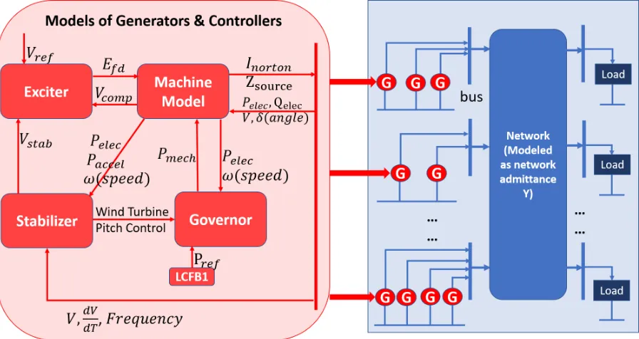
To assess the power system transient stability, dynamic simulation is performed to obtain time-domain trajectories after a fault in the system. We can analyze the trajectories with the state variables of the generators to determine the stability of the system. To perform the dynamic simulation, the behavior of the power system is analyzed thoroughly, and mathematical mod-els are developed to describe the dynamic behavior of various components in the system. The structure of the power system, as well as its data flow, is shown in Figure 2.1 [53]. Generally, this structure is used to conduct dynamic simulations. To understand this structure, we can see, at the system level, that there is an admittance network consists of generators, loads and the transmission lines. Mathematically, it can be interpreted as a linear or non-linear algebraic equation representing the network electrical measurements. When we look inside the generators, we can see that each generator is controlled by the exciter, stabilizer, and governor. The mod-eling of the generator is also a research topic in power system study, but will not be a focus in this dissertation. However, to better evaluate the dynamic simulation computing performance, the generator model with industry-level complexity will be implemented. Generally speaking, the generator model is described as a series of first-order differential equations.
Given the network and the generator model together shown in Figure 2.1, we can mathe-matically describe the system dynamics as Eq. 2.1, wherexrepresents a vector of dynamic state variables such as generator rotor angles, speeds or flux, as well as the dynamic state variables in exciters, governors and power system stabilizers, andurepresents a vector of network variables such as the magnitudes and phase angles of the bus voltages. We will introduce each one of the equation in Eq. 2.1 in the next, concerning generator models and the network electrics.
˙
x=f(x, u), 0 =g(x, u)
Figure 2.1: Flow Chart of a Generator and Its Controller Module, Together with the Admit-tance Network for Dynamic Simulation
Generator Models
As is mentioned earlier, in the industry, generators are typically modeled with its controllers, which can be a series of differential equations. In our studies, we will choose one such example to evaluate our computation performance. To make comparisons, we will also implement the classical model for the generator, which is more widely used for simplicity. The classical model is as simple as a second-order differential equation. See Eq. 2.2.
˙
δ(i)=ωB(ω(i)−ω0), ˙
ω(i)= ω0
2H(i)[Pm(i)−Pe(i)−D(i)(ω(i)−ω0)]
(2.2)
x in Eq. 2.1 only include rotor speed and angle, i.e.,
x= [δ(1), ω(1), ..., δ(i), ω(i), ..., δ(N), ω(N)] (2.3)
As is shown in Figure 2.1 above, the detailed model typically consists of a machine model, together with its controller modules such as exciter, governor and stabilizer. The detailed model or the one with industry-level complexity we use in this dissertation is referenced from work contributed by the Pacific Northwest National Laboratory(PNNL) [17], where they have demon-strated detailed illustrations and the expressions for the differential equations. We will use this as an example to show the detailed generator model, which is quite similar but not exactly the same as the example given in [17].
a Machine Model
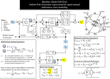
In commercial packages, a variety of machine models exist to describe the dynamics of mass rotation and the interaction between the machine stator and the power network, e.g., for the steam turbine, wind turbine or hydro turbine. In this example, the detailed flowchart is demonstrated in Figure 2.2 [52].
b Exciter Model
Exciters are used to provide transient voltage support in case of disturbance to restore bus voltages by providing a signal of field voltage, Efd, to the generator. There are over 50 types of excitation system models commonly used in commercial software packages. Each of them represents a physical control system with different levels of complexity. The number of state variables and actual control, therefore, can vary, depending on their parameter settings [17]. In our implementation, we use the ESST1A and ESST1A GE as the example for exciter model, shown in Figure 2.3 [52].
c Governor Model
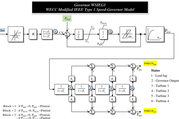
Governors are used to regulate machine rotation frequency by providing a signal of me-chanical power, Pm, to the machine model. In our implementation, WSIEG1 model is used for our governor, details shown in Figure 2.4 [52].
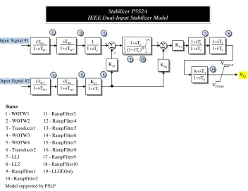
d Stabilizer Model
Machine Model GENSAL
States:
1 – Angle 2 – Speed w 3 – Eqp 4 – PsiDp 5 – PsiQpp
Machine Model GENSAL
Salient Pole Generator represented by equal mutual inductance rotor modeling
𝛿̇=𝜔 ∗ 𝜔0
𝜔̇=21𝐻 �𝑃𝑚𝑚𝑚ℎ1 +− 𝐷𝜔𝜔 − 𝑇𝑚𝑒𝑚𝑚�
𝜔̇=21𝐻(𝑃𝑚𝑚𝑚ℎ− 𝐷𝜔 − 𝑇𝑚𝑒𝑚𝑚) Mechanical Swing Equations
𝜔 = per unit speed deviation, so 𝜔= 0 means we are at synchronous speed and 𝜔= 1 would mean it’s spinning at double synchronous speed 𝜔0 = synchronous speed 2𝜋𝑓0where 𝑓0 is the
nominal system frequency in Hz
Note: If option Ignore Speed Effects in Generator Swing Equation is true, then instead use
1 𝑇𝑑𝑑′𝑠 1 𝑇𝑑𝑑′′𝑠 𝑋𝑑′′− 𝑋𝑒 𝑋𝑑′− 𝑋𝑒 𝑋𝑑′− 𝑋𝑑′′
(𝑋𝑑′− 𝑋𝑒)2
𝑋𝑑′− 𝑋𝑑′′ 𝑋𝑑′− 𝑋𝑒 𝑋𝑑− 𝑋𝑑′ ∑ 𝑋𝑑′− 𝑋𝑒 ∑ ∑ ∑ 𝐼𝑑 𝐸𝑓𝑑 ψ𝑑 ′′ 1 𝑇𝑞𝑑′′𝑠 ∑ + + + + + + + _ + _ _ _ _ 𝑋𝑞− 𝑋𝑞′′ 𝐼𝑞 ∑ + 3 4 5 ψ𝑑 ′ ψ𝑞 ′′ 𝐿𝑎𝑑𝐼𝑓𝑑 1 2 𝐸𝑞′ 𝐼𝑟+𝑗𝐼𝑖 𝑅𝑎+𝑗𝑋𝑞′′ ψ𝑞=ψ𝑞 ′′− 𝐼 𝑞𝑋𝑑′′ ψ𝑑=ψ𝑑 ′′− 𝐼 𝑑𝑋𝑑′′ 𝑇𝑚𝑒𝑚𝑚= ψ𝑑𝐼𝑞−ψ𝑞𝐼𝑑 Electrical Torque Field Current To Exciter 𝑍𝑠𝑑𝑠𝑟𝑚𝑚=𝑅𝑎+𝑗𝑋𝑑′′
𝑌𝑠𝑑𝑠𝑟𝑚𝑚=𝑅 1
𝑎+𝑗𝑋𝑑′′=𝐺+𝑗𝑗
𝐕=𝑑𝑑𝑑ψ=𝑗(1 +𝜔)�ψ𝑑 ′′+𝑗ψ 𝑞 ′′�
𝑉𝑑+𝑗𝑉𝑞= �−ψ𝑞 ′′+𝑗ψ𝑑 ′′�(1 +𝜔)
𝐼𝑑+𝑗𝐼𝑞= �𝑉𝑑+𝑗𝑉𝑞�(𝐺+𝑗𝑗)
𝐼𝑟+𝑗𝐼𝑖=�𝐼𝑑+𝑗𝐼𝑞�𝑒𝑗(𝛿−𝜋2) Network Interface Equations
Convert to Network Reference
a-axis b-axis c-axis d-axis q-axis 𝛿 a
c b
𝜋 2− 𝛿
Treatment of 𝑅𝑚𝑑𝑚𝑐and 𝑋𝑚𝑑𝑚𝑐
When specified, the compensated voltage fed as an input to the excitet is calculated as: 𝑉𝑚𝑑𝑚𝑐 = �𝑉� −𝑡 (𝑅𝑚𝑑𝑚𝑐+𝑗𝑋𝑚𝑑𝑚𝑐)𝐼��𝑡
Exciter ESST1A and ESST1A_GE R sT + 1 1 Σ REF V + − + Σ + − A V FD E Exciter ESST1A
IEEE Type ST1A Excitation System Model
1 A A K sT + AMAX V AMIN V 1 F F sK sT + 0 − HV Gate IMIN V ( )( )
( )( 11)
1 1 1 1 C C B B sT sT sT sT + +
+ + HVGate
OEL V LV Gate I V T RMIN V V
T RMAX C FD V V -K I
LR K Σ IFD
LR I Alternate Stabilizer Inputs Alternate UEL Inputs + + − + C E F V 3 4 5 1 2 A t 1 - V
2 - Sensed V
3 - LL 4 - LL1 5 - Feedback States
Support in PSLF and PSSE. Different integer codes for VOS (or PSSin), and UEL codes
VUEL ESST1A: UEL=1 ESST1A_GE: UEL=2
VUEL ESST1A: UEL=3 ESST1A GE: UEL= -1
VUEL ESST1A: UEL=2 ESST1A_GE: UEL= +1 VS ESST1A: VOS=1 ESST1A_GE: PSSin=0 VS ESST1A: VOS=2 ESST1A_GE: PSSin=1
Governor WSIEG1
Governor WSIEG1
WECC Modified IEEE Type 1 Speed-Governor Model
Δω err 1 db 4 1 1+sT
1
K
5 1 1+sT
3
K
6 1 1+sT
5
K
7 1 1+sT
7
K
Σ Σ
2
K K4 K6 K8
Σ Σ Σ Σ HP PMECH LP PMECH + + + + + + + + + + + + M1 P M2 P GV N O U C U 1 s MAX P MIN P 2 db GV P − − 3 1 T K 2 1 1 1 sT sT +
+ CV Σ
+
Model supported by PSSE
GV1, PGV1...GV5, PGV5 are the x,y coordinates of NGV block 1
6 5
3 4
2
1 - Lead-lag 2 - Governor Output
3 - Turbine 1 4 - Turbine 2 5 - Turbine 3
6 - Turbine 4 States
MIN MIN MAX MAX MIN MIN MAX MAX Iblock 1 : if P =0, P =Pinitial Iblock 2 : if P =0, P =Pinitial Iblock 3 : if P =0, P =Pinitial
: if P =0, P =Pinitial
= = =
𝑃𝑟𝑟𝑟
Stabilizer PSS2A
Stabilizer PSS2A IEEE Dual-Input Stabilizer Model
+ + Σ STMIN V STMAX V
Input Signal #2 W1 W1 sT 1+sT 6 1 1+sT W2 W2 sT 1+sT W3 W3 sT 1+sT S2 7 K 1+sT W4 W4 sT 1+sT S3 K N 8 M 9 1+sT (1+sT ) + − S1 K 1 2 1+sT 1+sT 3 4 1+sT 1+sT ST V
A B S4
Model supported by PSLF
Model supported by PSSE without T ,T lead/lag block and with K =1
A+sT 1+sT A B S4 K Σ 7 8
1 2 3
4 5 6
Input Signal #1
1 - WOTW1 11 - RampFilter3
2 - WOTW2 12 - RampFilter4 3 - Transducer1 13 - RampFilter5 4 - WOTW3 14 - RampFilter6
5 - WOTW4 15 - RampFilter7 6 - Transducer2 16 - RampFilter8 7 - LL1 17 - RampFilter9
8 - LL2 18
States
- RampFilter10 9 - RampFilter1 19 - LLGEOnly 10 - RampFilter2
19 9 − 18
Each module listed above is implemented in our simulator, as the detailed model. In reality, there are a variety of models for the machine, exciter, governor and the stabilizer depending on their wide variety of types in the world. In [52], it presents an example of how they are modeled in PowerWorld, which is a commercial simulator. As mentioned, since our primary focus will be on high-performance computing, we will not expand the discussions on generator modeling, nor the model technical details. Rather, we will focus on demonstrating the competence of our simulator for faster than real-time dynamic simulation. The motivation of presenting the detailed generator example is to evaluate the performance of industrial generator model with similar complexity as the example in [17].
Network Electrics
As we have discussed the various generator models above, which is shown as the differential equations in Eq. 2.1, there is another important part in that equation, which represents the network electrics, including the transmission line connectivity, the magnitudes and phase angles of the bus voltages, and the current the generators injecting into the network. It is typically modeled using algebra equation. See Eq. 2.4
I =Y ·V (2.4)
WhereIis the vector of current injection from the generators, which is acquired by applying Norton Equivalent to the generator voltage output and the internal impedance;Yis the network admittance matrix which also includes generator equivalent admittance and the equivalent static load admittance, with the dimension of the total number of buses; V is the vector of the bus voltages. For computation efficiency, we regardYas a linear matrix. Also as we know, there are several types of load models, including the constant ZIP model, frequency/voltage-dependent models, and composite load models, etc. For better computation efficiency we adopt the constant impedance model for all the loads, and hence the load information is contained in Y in the system.
Figure 2.6: Distribution of Node’s Degrees incase9241pegase
the median of all the transmission lines admittances, as the distribution of transmission lines might have a wide range numerically. Thus mathematically, Y can be represented as:
Yi,j =
branch admittance between Node iand Nodej, i6=j
−PN
i=1,i6=j(Yi,j−Yid), i=j
(2.5)
In the remaining of this subsection, we explore the statistics of the power system matrix Y in brief.
Statistically, the number of nodes connected to generators is around 15% to 25% among all the nodes, and their correspondingYidare much greater than normalYij. Meanwhile, we treated our loads as constant impedance model whose corresponding admittancesYid are generally nu-merically close to the transmission lines, hence the matrix will be strictly diagonally dominant, with the diagonal items numerically no smaller than the sum of their corresponding rows or columns. Also according to the definition of Yij, it is easily inferred that it is a symmetrical matrix. Meanwhile, due to the very sparse connection of power system, MatrixY is very sparse: typically each node has 3 to 5 connections to other nodes [15]. In Figure 2.6, an IEEE test case is shown as an example of the distribution of degrees for its nodes.
In the IEEE test files, as Yid values are not given, the only way we can do is to randomly generate them based on their rules depending on whether the nodes are connected to generators or loads. If connected to generators, then their correspondingYid values will be randomized 10 times larger than the median of all the transmission lines’ admittances in the system, with some random deviations. Since the transmission lines’ admittances have a relatively wide distribution, we have to choose some mid-ranged value as the baseline. In Figure 2.7, we show the distribution of transmission lines’ admittances.
Figure 2.7: Cummulative Distribution Function of the Magnitude of Transmission Lines’ Impedances(Zoomed In)
0.01 and 0.02. If we choose 0.05 as our baseline, then its magnitude will be above 85% trans-mission lines’ impedance, or in other words, its corresponding admittance is smaller than 85% of all the transmission lines. It is a conservative estimation as the actual diagonal dominance of the matrix is likely to be better than that, as their corresponding internal admittances are likely larger than our estimation.
Finally, it is emphasized that all the items in the equationY V =I are either complex values since the transmission lines contain both resistive and reactive components or zero if there’s no connection and that the generators current source are also complex values, indicating both their magnitudes and phases.
2.2.2 Simulation Process
twice. To ensure its numerical accuracy, we typically set the simulation step interval ∆T as 0.005 seconds between each calculation of the modified Euler’s method. As we simulate 10 seconds for real-time, we should repeat the modified Euler’s method for 2,000 times.
2.3
Real Time Challenges
As is explained in the previous sections, power system dynamic simulation consists of the numerical integration of swing equations for generator state variables, and the linear system equation for network electrics. Due to the intensive computations involved, the simulation tends to be very time-consuming. On the other hand, the dynamic transient of the power system towards a fault can have a drastic fluctuation within a few seconds, which is already a very stringent time duration.
Today, explicit integration method is widely used for power system transient stability anal-ysis. The 2nd order of the modified Euler method is especially popular as mentioned above. While the differential equations for state variables are more accessible to parallel since the generators are intrinsically decoupled, the computations of different generator state variables are independent. However, the system equation to solve bus voltages can be time consuming especially for large system size. Conventional solutions to the linear system such as L-U direct solver is computationally expensive when manipulating the matrix decomposition, and highly sequential in computation when manipulating the back-substitution. Popular iterative methods, such as Jacobi and Gauss-Seidel methods, converge slowly. There are also waveform relaxation methodologies to decouple the matrix, and iterative methods to solve the network electrics and the generator differential equations, but there are two major drawbacks: (a) the convergence of such iterative method is yet to improve to get real-time; and (b) there are not any rigorous mathematical derivations to handle matrix topology change due to the transmission line fault. Thus, the key to solving the real-time issue is to find an efficient way to compute the linear system equation, as well as being capable of handling the matrix topology change efficiently.
To be more specific, as is mentioned in the Subsection 2.2.2, we have a step-length of 5ms for each time stamp, and in each time stamp, we have to compute two steps of the Modified Euler’s Method. Hence, even if we ignore the timing on the differential equation for generators, to achieve real-time, each step of linear matrix equation must be solved within at most 2.5ms.
2.4
Prior Work
further research on how to accelerate systems with large scales. Research in accelerating dynamic simulation has been categorized into analog [21–24, 41, 45, 46] and digital approaches [2, 4–6, 13, 16, 17, 27, 30, 31, 33–35, 56, 58, 60, 61].
2.4.1 Analog Approaches
The concept of analog computer dates back to the 1960s [36]. Even today’s digital computers have the significant stronger computational capability, the bottleneck in parallelization or iter-ative convergence makes the faster-than-real-time anticipation challenging when it comes to the power system dynamic simulation. To increase the parallelization, analog researchers attempted the analog computer that originated from the idea that the electrical signals can propagate in-trinsically in parallel. The analog architecture for power system dynamic simulation was first introduced in [24], followed by the phasor emulator [22] and alternating current(AC) signal emulator [45, 46]. To achieve better scalability, Fabre et al. proposed a series of mixed-signal emulators with DC signals in their purely-resistive networks [21, 23, 41]. In their proposed solu-tion, they applied numerical approximations to the admittance of the networks and divided the complex number computations into the real and imaginary components to use purely resistive networks to collect bus voltages, while using Field Programmable Gate Array(FPGA) for state variables. They were able to achieve a 1,000 times faster-than-real-time when simulating a 100-bus system transient. However, the scalability issue still makes implementation very difficult for larger systems due to chip size, interconnections and quadratically increased signal propagation delay [20].
2.4.2 Digital Approaches
Digital approaches can be further categorized into parallel-in-space and parallel-in-time [29]. For further simulation speed-up,parallel-in-spaceandparallel-in-timecan be used together(e.g.,
waveform relaxation). Theparallel-in-spacealgorithm takes advantage of the natural decoupling
of the power system topology and break down of the original system into multiple workloads to be processed among processors. One example is the parallel Newton type method discussed in [13]. Recently, study in terms of theparallel-in-space was categorized into Schur-complement based method [5, 6, 60, 61] and Schwarz alternating method [2] [56]. In the Schur-complement based method, a reduced system model must be formulated to calculate the interface variables followed by naturally decoupling the subproblems, which is a ”direct” method, while in Schwarz, the interface variables are iteratively updated after the associated subproblems are solved, until a global convergence is achieved.
The parallel-in-time algorithm solves multiple time steps simultaneously. The idea was
in [31] [16], which decomposed the whole system into sub-systems to process in parallel, with the relaxation-based iterative method. In [27], the Parareal algorithm was proposed to divide the time evolution problem into a series of problems on smaller step intervals, using a coarse approximation to make an initial guess, and updating the solution of each small step in parallel. All methodologies mentioned above covered a variety of ways to decouple the network equation problems and parallel the computation. Among the methodologies, accomplishments are made regarding faster-than-real-time anticipation. Examples are [17, 30, 33–35] by the re-searchers in the Pacific Northwest National Laboratory(PNNL). Block Gauss elimination, L-U and Woodbury matrix identity methods were utilized, with the help of HPC technology. By using OpenMP to implement their approach in parallel, a 9.04-second simulation on 16,072-bus, 2,361-generator system for 30-second real time was achieved in [34] [35]. However, since their methodology was still based on the classic L-U method, the matrix decomposition was still time-consuming, which took over 4 seconds according to their efforts (i.e., the first 4-second post-fault dynamics could never be simulated in real time). The other example in [58] [56] used Parallel-General-Norton with Multiple-port Equivalent(PGNME), to precondition the iterative matrix and enhance the convergence of the iterative computation based on the Schwarz alter-nating method. A nearly 10 times faster-than-real-time performance could be achieved when handling very large system with 45,552 buses and 7,167 generators on a state-of-art HPC cluster ”Shadow II”. Their methodology could simulate very large systems in real time, albeit, they did not have a rigorous mathematical proof to ensure the preconditioning performance given a fault-triggered topology change in the admittance matrix (i.e., it did not always guarantee faster-than-real-time when simulating transmission-line fault scenarios).
As the state-of-the-art methodologies are reviewed with their advantages and drawbacks, we decided to focus on designing a novel simulator that can achieve faster-threal-time an-ticipation that could be competent to handle minor topology change while maintaining faster-than-real-time simulation. Also, compared to the wide-spread HPC platform solutions, we were also seeking for a more economical choice of the implementation platform.
2.5
GPU Architectures and CUDA Programming
In this dissertation, the GPU architecture will be utilized to accelerate the dynamic simulation for data parallelization, programmed with C++/CUDA.
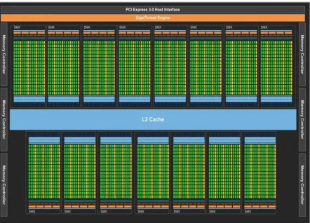
Figure 2.9: Architecture of NVIDIA K40 GPU
complexity and the massive integration of the processor. On the other hand, based on the Amdahl’s Law [28], multi-core/many-core architectures become increasingly popular, which is widely used in parallel computing. As a many-core architecture, GPU typically has hundreds or even thousands of cores along with massively distributed memory architectures. Given its parallel architecture, GPUs are becoming more and more prevalent in the cutting areas of both academia and industry.
Figure 2.12: Comparison of GPU and CPU Architectures [54]
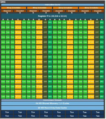
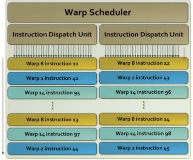
to be issued and executed concurrently. It also has eight instruction dispatch units, allowing two independent instructions per warp to be dispatched each cycle [49]. The mechanism of the quad warp scheduler is shown in Figure 2.11. In K40, SMX can issue up to 64 active warps for a total of 15×64 = 960 active warps. The back-end of each SMX contains 192 cores(6 warps) for integer and single-precision(SP) floating number arithmetics, 64 cores(2 warps) for double-precision(DP) floating number arithmetics, 32 cores(1 warp) of load-store units and 32 cores(1 warp) of special function units. Hence a total of 16 concurrent warps could be executed in each SMX. In a total of 15 SMXs, a maximum number of 2,880 SP floating number arithmetics or a theoretical maximum of 7,680 different types of arithmetics could be executed concurrently. The memory architecture, including shared memory, L1-Cache, the read-only data cache, L2-Cache, DRAM, etc, is connected to each SMX with the interconnection network. Besides, for NVIDIA GPUs the main memory is divided into multiple banks, and each bank can only address one dataset at a time. With the help of multiple banks, the GPU memory typically has very large memory bandwidth.
or thousands of cores. Despite the longer latency in its ALU operation as well as the memory access, the latency will be hidden by the uninterrupted data flow. Thus, high throughput is achieved.
The representative GPU kernels include the matrix-vector multiplication(MVM) and matrix multiplication. When matrix size is large, there are massive amounts of multiplications as well as the reductions in both kernels. Despite the massive operations, they all belong to the same type. Therefore, the data of the matrix will be divided into thousands of partitions, which are processed by the massive number of GPU cores in parallel, under the same instruction. In this case, the data parallelization is achieved.
CUDA is a parallel computing platform and application programming interface(API) model created by NVIDIA, and it allows software engineers to use GPU for general purpose process-ing. The platform is designed to work with common programming languages such as C/C++, Fortran, Java, Python, Matlab, etc. The hardware environment of CUDA platform includes the combination of host and device. The host typically includes the CPU, CPU cache, main memory, and other supporting architectures. It primarily handles interrupts, controlling and communication information. The device refers to the GPU or maybe multi-GPU architecture, which is responsible for the compute-intensive applications. The source code of CUDA consists of both the host and device codes. The NVIDIA C Compiler(NVCC) parses the codes into two partitions, one executed by the host and the other by the device. The detailed compilation process of NVCC is shown in Figure 2.13.
Figure 2.14 shows the processing flow on the CUDA platform. As is shown in the figure, data is copied from the host main memory to the device memory or the GPU memory. Then, CPU initiates the GPU compute kernel, and the GPU cores execute the kernel in parallel. Finally, the resulting data from the device is copied to the main memory.
Chapter 3
A Feasibility Evaluation on Analog
Approach
In Chapter 2 we reviewed the analog approaches mostly proposed by the research group in EPFL. Considering the better scalability presented in that chapter compared to the AC analog emulation, we will further evaluate the scalability of their mixed-signal approach.
3.1
Introduction
A board level implementation of a DC emulator is presented in [21, 40, 41]. The network is implemented using analog methods while the generators and loads are digitally modeled. Seen in Figure 3.1, there would be four types of chips: DAC arrays, ADC arrays, a mesh of pro-grammable resistors, and the FPGA board modeling generators and loads. The digital and analog portions are connected by ADCs and DACs. The network is built using calibratable potentiometers to model the reactive elements only in one network and real elements only in a separate network. Calibration is conducted against high precision resistors at each node. Analog switches are used to change the topology. A 57-bus system was built on a 4 board stack. It achieved 1000 times faster than real-time. It is called the Field Programmable Power Network System (FPPNS). Reference [21] describes a 3-D board stack potentially implementing 96 buses and 336 branches (A single board potentially implements 24 buses and 84 branches). For each emulation step, the FPGA computation time took 200 ns, the ADC took 200 ns, while the DAC took 400 ns and the grid response time took 200 ns.
The question addressed in this report is whether a large scale version of the FPPNS can be built using IC technology. The scale is intended to be of the order of 10,000 buses, and its emulating performance should be at least FTRT.
Table 3.1: Percentage of Nets That Do Not Meet the Assumption That Permits Separation of Real and Imaginary Networks
Benchmark % of lines with Xij >> Rij
IEEE-30 17%
IEEE-89 59%
IEEE-118 12%
IEEE-300 27%
IEEE-2746 27%
IEEE-9241 41%
imaginary arrays hinges on the assumption thatRij << Xij. An analysis on the IEEE bench-marks will be conducted to validate this assumption.
Second, as the scale of such an emulator grows up, it can result in an RC delay chain within the large resistor array according to the Elmore Delay Model [20]. More experimentations must be conducted to explore its scalability upon emulating the 10,000-bus system.
Third, the resistors would need to be calibrated, which would take one hour. The calibration is not perfect, leading to the emulation inaccuracy.
Finally, mapping real networks onto the programmable resistance mesh requires that some branches in the mesh be configured as shorts. A perfect analog short is not possible with CMOS technology, introducing an additional error.
3.2
Numerical Assumptions on Transmission Lines
3.3
Chip Scales of FPPNS
In this section, we will focus on the scalability of the FPPNS, including its estimated device number, total chip area, signal delay issue as well as other electrical issues when the emulator is expected to scale up to simulate over 10,000-bus system.
The mixed signal core of the chip-scale FPPNS would include the following components:
ADCs and DACs at the interfaces.
Reconfigurable resistor network consisting of calibratable resistors at each branch
Calibratable resistors
Calibration support
3.3.1 ADCs and DACs
Reference [21] describes using 12 bit resolution ADCs and DACs, operating at 5 MS/s. These are certainly feasible and probably best purchased as IP blocks. Let’s assume a total of 2,000 generators for a 10,000-bus system, which is a practical number. For each generator, there is a pair of ADC/DAC coupled to one network. Taking both reactive and resistive networks shown in [21], a total of 8,000 ADCs and DACs are needed for a 2,000-generator system. The power of each ADC/DAC can be as low as 0.2 mW, though 1 mW is more typical. Thus the total power budget for these is less than 8 W, which is reasonable. A typical area for a successive approximation ADC in 130 nm is 0.1 mm2. Thus 8,000 ADCs would occupy 800 mm2 (or 28mm ×28mm), which is acceptable. Overall, the ADCs and DACs are feasible upon further scaling-up.
3.3.2 Reconfigurable Resistor Network
The resistor array and their control and switching present the main challenge for a chip-scale FPNNS. It appears in the FPNNS that a mesh network was built with connected diagonals Figure 3.2. Note that natively, this supports a maximum of degree at each bus of 6 branches. In analyzing the IEEE benchmarks, it was noted that some buses had up to 40 branches connected to them. Thus to map such a network onto a mesh with a degree of 6, it is necessary to support branches with zero resistance, so that high degree nodes in the electrical network can be achieved by shorting together multiple nodes in the emulator.
Figure 3.3: On-chip Programmable Resistor
the real network. Reference [21] indicates that the resistors are 8-bit programmable, giving a tuning range of 1:28or 1:256. Analysis of the IEEE benchmark data indicates a need for a larger turning range of 1:103 or even 1:104, equivalent to 10 bits of programmability. High linearity is also needed according to [21]. In the sections below, we will expand on how to build the on-chip programmable resistors.
Programmable Poly Sheet Resistor
One way to build an on-chip programmable resistor is shown in Figure 3.3. The fixed resistors are built using high ohmic polysilicon resistors. According to the datasheet published by Altis semiconductors, the high ohmic poly resistor density is 3kΩ/µm2. (Public domain data is used in this report, to prevent disclosure of proprietary fab data.) The switches are built using nFETs.
Unfortunately, the NFETs are not the ideal (zero on-loss) devices. Assuming a 130 nm process with an Ion of 415 µA/µm of gate width, then a 10 µm wide gate has an Ron of 200 Ω. To minimize the impact of this high Ron on the resistor reconfigurability, the resistor itself should be at least 10 times this resistance. In other words, the smallest resistance in this network should be 2 kΩ and the largest 1 MΩ given 10 programmable bit. These resistors would be built using arrays of identical resistors arranged in series, as shown in Figure 3.3.
or 512 unit resistors for the most significant bit(MSB). In this case, the total number of unit resistors for each programmable resistor array is 1023. We use 2kΩ for the least significant bit (LSB) resistor to minimize electrical issues. Based on the typical poly sheet resistance of 3 kΩ/µm2, the unit resistor requires 0.67 µm2. Thus the whole array requires 682 um2 of poly. With overhead for the nFETs, spacing rules, and the flip-flops that store the switch settings, empirically at least 5 times this area would be needed or approximately 3,410 um2, which is a footprint of 0.058mm × 0.058 mm. This translates into 293 resistors per mm2, or 273 mm2 of silicon for all 80,000 resistors (16.5 mm x 16.5 mm).
Since the nFET drains and sources are capacitive, this resistor chain acts as an RC delay chain when a transient is fed to the input. Each nFET would present about 1 fF of combined drain-source capacitance. The formula for the RC time constant of an RC chain is
τ =PN
i=1(RiPij=1Cj)
The delay model equation indicates a quadratic increase of signal propagation time in pro-portion to the total number of nodes in an RC-tree. To give an example, assume a chain of 100 resistors, i.e. 100 branches in the network end to end, which is likely to happen in a 10,000-bus power system. In this case, each resistor will see a load of 10 fF, and with the average resistance being 0.5 MΩ; as a result, the RC time constant across the entire network would be 25,250 ns. This needs to be compared with 200 ns in the FPPNL. Even if we ignore the time elapsed in the digital and analog-digital conversion modules, the emulation time step would increase from 1 us in the case of the FPPNL to 26 us. Instead of 100x real time, this system would at best achieve 40 x real-time (where real time is 1 ms per step [21]). It could be worse than this if the needed resistances are high and/or the longest spanning set of edges in the graph spans more than 100 branches. Analysis of IEEE-9241 benchmark indicates the potential for some nets spanning more than 140 branches. This delay is a serious threat to the viability of the mixed signal approach. Note, this is a very approximate calculation. The actual power system network can be better or worse.
One possible solution against the long spanning signal chain is to add some analog buffer to the output of each node or every few nodes. A possible candidate for such a buffer is shown in [12]. However, this would not support bidirectional current flow, and hence it cannot be applied to this implementation.
MOSFET Resistor
Figure 3.4: MOSFET Resistors
the poly resistor. However given the small signal nature of the emulation we are doing, a pure MOSFET approach probably would not be desired, as an individual FET resistor is not as linear as a film sheet resistor. However, the FET resistors are useful as described below.
Hybrid resistor
Another element that is needed is the low-loss analog switch. This is needed for two purposes: to create an open circuit when a branch is not used and to create a short to bypass an entire programmable resistor. Making a low-loss analog switch in CMOS difficult.
The suggested structure is to incorporate a pass gate FET resistor into a programmable poly resistor, e.g. replacing the 20 resistors with a pass gate FET resistor. Then this resistor can be turned completely off, changing that branch into an open circuit. Thus, the analog switch is combined with each branch resistor. Unfortunately, a pass gate resistor is not as linear as a two-element resistor, which is not as linear as the poly resistor.
Another use of the pass gate is to use it to bypass an entire programmable resistor to create a short. Unfortunately, it is difficult to create a perfect short. A reasonable target is to implement a short in the 50 Ω range. Note, this bypass short also increases the capacitive load on the circuit, which will slow it down further.
3.3.3 Calibration
The resistors have to be calibrated against an off-chip accurate potentiometer, like that used in [21]. It is reasonable that only a small number of these, for example 4 resistors, can be fitted on the board near the chip. Each would have dedicated pins connecting to the on-chip resistor array. Thus, the problem becomes one calibrating 80,000 programmable resistor arrays against 4 precise resistors. Each programmable resistor array has 10 binary resistors, 10 bypass nFETs, and one bypass pass-gate, all of which would have to be measured.
This is a non-trivial problem. The most obvious option is to connect each resistor and FET or pass gate in turn, via a lower resistance pass gate, to the ports that are connected to the off-chip potentiometers. The difficulty that arises is that the lower resistance pass gate will contribute to the resistance, with no way to accurately remove its effect, together with the impact of the wiring resistance. It can be mitigated by using large transistors for the pass gates. Thus, for example, the roughly 50Ω of wiring resistance and roughly 50Ω of pass gate resistance would be subtracted from the measured resistance. However, the pass gate resistance varies by +/-30%, so the resulting calibration would have an error of up to approximately +/-15Ω. This will cause a calibration error of up to 7%, but practically much less than that.
Calibration would be time-consuming. With 80,000 resistor arrays, 4 comparison resistors, and 21 sub-components values, a total of 80,000×21/4 = 420,000 steps would be required. With a digital controller, this is feasible but time-consuming. At 10 ms per step, it would take over one hour. Note recalibration would be needed every time the temperatures changes by more than 10◦C. This issue can be avoided by putting the chipset on a temperature controlled heated stage. It would be best to use an on-chip diode as the temperature measurement device.
3.3.4 Packaging
Figure 3.5: Overall Concept for Resistor Array
3.4
Conclusions
Chapter 4
A Preliminary Numerical Approach
Based on the Preconditioned
Richardson Iterative Method
4.1
Introduction
As discussed earlier, the difficulties for real-time simulation is the linear matrix solver. According to the analysis in the previous chapter, the analog implementation on an over 10,000-bus system can be challenging due to the scalability issues. Hence, a better chance exists in numerical solutions if we can design an algorithm with much lower arithmetic complexity and with high parallelization. As is shown in Figure 4.1, the linear matrix solvers can be categorized into direct solvers or iterative solvers. For direct solvers listed in Figure 4.1, the arithmetic complexity of solving the equation Ax = b are all O(N3), or its total number of arithmetic operations is cubically proportional to the dimension ofA. Even the sparsity of A does not help and won’t lead to a significant reduction of the complexity. Therefore, when the dimension of A is large, the direct solvers will be very inefficient to solve the system equation.
Figure 4.1: Classification of Solvers for Linear Systems
matrix without actually solving it if we choose to find a preconditioner for the stationary method. However, as is stated, the fault only occurs low-rank correction to the admittance matrix. We can take this advantage of this observation when approximating its preconditioner.
4.2
Convergence Analysis of Stationary Iterative Methods
To begin the analysis, we start with stationary methodologies. The most common methods include Jacobi, Gauss-Seidel, and Richardson methods. Given the systemAx=b, regardless of the differences among the methodologies mentioned above, all of their iterative expression can be represented as
x(n+1)=M ·x(n)+c (4.1)
where M and c are corresponding to Table 4.1.
In Table 4.1, D is the purely diagonal matrix of A, R is the purely off-diagonal matrix of A,U is the upper diagonal matrix of A,L∗ =A−U,I is the identity matrix.
Table 4.1: Corresponding M for different iterative methods
M c
Jacobi −D−1R D−1 Gauss-Seidel −L−1
∗ b L−∗1b
Richardson I−A b
the spectral radius of M is smaller than 1, or
ρ(M) = max λ∈ρ(M)
|λ|= lim n→∞||M
n||1
n <1 (4.2)
where λ represents all the eigenvalues of matrix M. Also according to the expression of Eq. 4.1, its not difficult to know that to get Eq. 4.1 converged to an accuracy of, the number of iterations required can be estimated as
N = logρ(M)= log()
log(ρ(M)) (4.3)
Given a group of experiment based on the IEEE test casecase1354pegase, we get the results shown in Table 4.2:
Table 4.2: Convergence by Different Iterative Method forcase1354pegase
ρ #Iter
Jacobi 10−5 0.9969 3714 Gauss-Seidel 10−5 0.9938 1857
Richardson 10−5 1.89×10⁴ Unable to Converge
The result shows that without preconditioning, the converge is too slow, or even unable to converge. However, due to their simplicity, as long as we can find a good preconditioner, it is still a promising approach to implement.
4.3
Preconditioned Richardson Iterative Approach on Handling
One-line Fault
Preconditioned Richardson Iterative Method. Given the post-fault system Y V = I, we can design a preconditionerP, such that
P Y ·V =P I (4.4)
As long as Eq. 4.2 is ensured, its iterative expression is shown as
V(n+1) =V(n)−(P(Y ·V(n)−I)) = (I−P Y)V(n)+P I (4.5)
where M =I−P Y. To ensure its convergence, the spectral radius of M should be smaller than 1; the smallerM is, the faster it can converge, as is explained in Eq. 4.3 [37]. The intuition of choosingP is to approximate the inverse ofY, but how closely P should be approximated? The ideal P is the inverse of Y, which is very inefficient to obtain. The other extreme case is to choose P as an identity matrix which is extremely efficient, but has no preconditioning effect. Therefore, we need to choose an approximation between these two extreme cases while considering both effectiveness and efficiency.
4.3.1 Preconditioner Design: Approximation of the Inverse
One candidate forP can be the inverse of the pre-fault matrixY0, which can be pre-processed before the simulation process and thus have no timing cost. Since only 4 items of Y0 changes after the fault, it is likely that the inverse of Y0, or inv(Y0) is close to the inverse of the post-fault matrix Y, or inv(Y). However, as we have further verified, such a preconditioning strategy has no guarantee of success under all possible cases. Hence, we further explore better preconditioning strategies.
To continue our discussion, we split the matrix in terms of “degrees of separation” to the faulted nodes, using the thoughts in the social network. Figure 4.2 gives us an outlook on how the nodes are split in terms of “degrees of separation”.
Now if the nodes’ index order, assign Y as a combination of sub-blocks as
Y =
Y11 Y12 Y13 . . . Y1n Y21 Y22 Y23 . . . Y2n
..
. ... ... . .. ... Yn1 Yn2 Yn3 . . . Ynn
N×N
(4.6)
Figure 4.2: Example of Mini-Social-Network Matrix Reordering
separation. Since each diagonal sub-block of Y can be mapped to one sub-block of our entire power system, it is easy to see that all of them are non-singular. Also, as the matrix is reordered based on degrees of separation, it is easy to see that some of the sub-blocks in Y are indeed zero matrices. Hence we get
Yi,j =
0, |i−j|>= 2 Yi,j, Otherwise
(4.7)
Concurrently, let’s consider a sub-block view of Y0−1 and Y−1, where we use the same sub-blocking strategy used in Eq. 4.6, shown below:
Y0−1 =
T0,11 T0,12 T0,13 . . . T0,1n T0,21 T0,22 T0,23 . . . T0,2n
..
. ... ... . .. ... T0,n1 T0,n2 T0,n3 . . . T0,nn
N×N
(4.8)
Y−1=
T11 T12 T13 . . . T1n T21 T22 T23 . . . T2n
..
. ... ... . .. ... Tn1 Tn2 Tn3 . . . Tnn
N×N