Diectromagnetic interrogation techniques for damage detection

(1)

for

Damage Detection

H. T. Banks and M. L. Joyner

Center for Research in Scientific Computation

North Carolina State University

Raleigh, NC

and

Buzz Wincheski and W.P. Winfree

Nasa Langley Research Center

Hampton, VA

(2)

Electromagnetic Interrogation Techniques for

Damage Detection

H. T. Banks

, Michele L. Joyner

, Buzz Wincheski

, and William P. Winfree

Center for Research in Scientific Computation, North Carolina State University, Raleigh, NC 27695

NASA Langley Research Center, Hampton, VA 23681

Abstract.

This paper introduces a computational method for use with eddy current damage detection tech-niques. To identify the geometry of a subsurface damage, an optimization algorithm is employed which requires solving the forward problem numerous times. In order for the method to be effective in a practical setting, i.e., in real-time applications, the forward algorithm must be extremely fast and accurate. Therefore, we have chosen an approach based on reduced order Proper Orthogonal Decom-position (POD) methods. This allows one to create a set of basis elements using snapshots with either numerical simulations or experimental data. The data is organized in an optimal way allowing one to use a reduced number of basis elements, resulting in a fast algorithm while still obtaining an accurate approximation to the solution. We first derive the model associated with the chosen nondestructive evaluation (NDE) technique and prove some well-posedness results for the model. We then introduce the proposed computational methodology and test it on both numerically simulated data as well as experimental data obtained from a GMR (Giant Magnetoresistive) sensor. The results demonstrate that the method is extremely efficient and accurate.

1 Introduction and Problem Formulation

As technology continually advances, the field of nondestructive evaluation is in continual need of new techniques and instruments to improve the accuracy and efficiency of locating and characterizing sub-surface damages. We attempt to develop a new methodology which, when coupled with already existing techniques, can help decrease the total computational time required to detect and explicitly characterize a damage within a material. This is necessary in practical settings where the methods must be fast and ac-curate, producing real-time results. Given data obtained from a measuring device such as the GMR (Giant Magnetoresistive) sensor, we seek to locate and parameterize the damage while minimizing the amount of time required to complete this task. To this end, we formulate and develop an appropriate model used in describing the variation in the data as a function of a damage within the sample and present computational methods along with numerical results to support the efficacy of our approach.

1.1 Description of the Test Problem

(3)

magnetic field perpendicular to it that in turn produces a current within the sample, called an eddy current. When a flaw is present within the sample, the flaw disrupts the eddy current flow near the flaw and this disturbance is manifested in the magnetic flux density detected by the measuring device.

Figure 1: Inspection Process using a SQUID

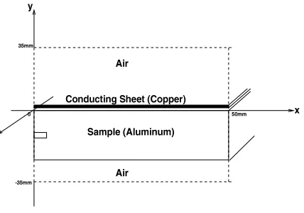
For illustrative purposes, we will assume uniformity along the width ( direction) of the sample,

therefore reducing the three-dimensional problem to a two-dimensional problem. To test the feasibil-ity of reconstructing the geometry of the damage, we consider the damage (which we shall refer to as a “crack”) to be rectangular in shape. In other words, we assume the crack, located at a certain depth within the sample, has a fixed length and thickness. To further simplify the test problem, we disregard the boundary effects of the materials in the direction (sample length) by assuming an infinite

sam-ple and conducting sheet in that direction. Because we are considering materials of infinite extent, we will construct our forward problem by focusing on a small “window”, called our computational domain

"!#$!&% ')(+*%, "!-.!-*%, $/ , centered such that the left boundary

of the computational domain, at location

, is positioned in the center of the crack in the direction,

i.e., the crack is symmetric through the plane at

. A schematic of the resulting two-dimensional

problem is depicted in Figure 2 where it is assumed that the sample (which is 0 thick) is composed

of aluminum, the conducting sheet (which is2143) thick) is made up of copper and the crack is centered

in the direction around the center of the sample (i.e., around

(53) ).

6 7 8 9 :; <= :> 8 ?@ > 8 A B

C DCEE

F G @H >IJ?@K 6 L;;J <F G 9 9; MA

= ?M

NO DEE

O

DEE

= ?M

P

Q

(4)

4 Electromagnetic Interrogation Techniques for Damage Detection

1.2 Resulting Equations for the Test Problem

In our computational efforts, we employ the use of the software package Ansoft Maxwell 2D Field Sim-ulator. Therefore, our equations are formulated to correspond to those used by the software. (For a full derivation of the resulting equations, see [3].) Although the GMR sensor measures the magnetic flux den-sity above the sample at a certain location, our equations are formulated in terms of the magnetic vector potentialR , where all the field quantities are assumed to be phasor quantities [4, 5, 6]. However, one can

easily obtain the resulting magnetic flux densityS through the relationship SUTWVYX$R .

Using Maxwell’s equations in conjunction with Ohm’s law and constitutive laws, we obtain an equation for the magnetic vector potentialR given by

VYX

Z [

\^]`_abdc VYX'R

]e_afbdchg

T

]jik]e_ab2cmloneprqcs]

R

]e_ab2cut

Vwv

c x_ab.y{z|a

(1)

where \

represents the magnetic permeability, i

represents the conductivity,p

is the angular frequency, andv is a scalar potential.

Since Eq.(1) contains two unknowns,R andv , an additional equation is needed to uniquely determine

the solution forR . For this we use an integral constraint given by

}s~j

T

~u TW

~j

]ei^]e_afbdcmlnjprq]`_abdccs]

R

]e_ab2cut

Vwv

c

u (2)

between the total current

}s~j

flowing in the conducting sheet (cs) and the total current density within the

conducting sheet. This is the second equation used in the software package Ansoft Maxwell 2D Field Sim-ulator which we use in our computational efforts. However, this only gives us equations which completely describe the magnetic vector potential and electric scalar potential in the conducting sheet. Nonetheless, the conducting sheet is the only region in which a source current of the form

T

t+i

Vv is present

and hence is the remaining regions we intuitively assume there is no change in potential, in other words

VwvoY . This gives us appropriate equations in which the magnetic vector potential R can be uniquely

determined if appropriate boundary conditions onR are specified.

In Section 1.1 we assumed the sample was of infinite extent with the crack being symmetric in the _

direction. In other words on the_

boundaries, we assume the fields on both sides of the boundary oscillate in the same direction. To account for the even symmetry, we assign Neumann boundary conditions to these boundaries. In a similar manner, we assume the b

boundaries are “sufficiently far” away from the sample and scanning area so as to not effect the overall measurements. Indeed, as one moves farther away from the sample and conducting sheet, the magnetic vector potentialR tends to zero. Therefore, on the

b

boundaries we assign null Dirichlet boundary conditions. The magnetic vector potentialR is thus determined by

VYX

Z [

\^]`_abdc VYX$R

]`_abdchg

T

]jik]e_ab2cloneprq]e_afbdccs]htnjp

R

]`_ab2cut

Vv

c x_ab y'a

(3)

}s~j

T

~ju

T

~j

]ji^]`_ab2cloneprq]e_ab2cfc]htnjp

R

]`_abdct

Vv

c

(4)

and

Vv T&

x_aby'

(5)

with

R

]e_a)t+ ¡c

T T R

]`_a ¡c

VwR

¢¤£¦¥f§¨©

T T VªR

(5)

2 Well-Posedness

In this section we consider the existence and uniqueness of a weak solution to the above boundary value problem on a general domain given by

¯

°±³²´eµ¶·¶¸¹º»¼¾½,µÀ¿ÁÃÂªÄµÄµÀ¿ÆÅ®Ç¶·,¿uÁÃÂÈÄ#·.Ä#·É¿ÆÅ®Ç¡Ê

for which our test problem is a specific example. LetË

±&ÌkÍÉ´ ¯ °Î¹ andÏ ± ²Ð#º ËÒÑ ´ ¯ °Î¹ÓfÐÔ´eµ¶f·,¿uÁÃÂ¹k±ÕÖ± ÐÔ´eµ¶·É¿ÆÅ®ÇÉ¹×Ê

where we use the standard Sobolev space notation, ËÒÑ

´ ¯ °¹Ô±Ø²ÐÙºÚÌ Í ´ ¯ °Î¹Ö½ÛªÐÙºÚÌ Í ´ ¯ °Î¹×Ê

and note that we interpret pointwise evaluation of functions (along the boundary and elsewhere) in terms of a trace operator for which we suppress notation throughout this paper [7]. We denote byÜÞÝ

¶fÐßkà áãâ

ä

Ý

Ðæåç

the standard inner product inË and ÜèÝ

¶Ðæßféêà³áâ

ä

Û

Ýë Û|Ðæåç

the (ËÒÑ-equivalent) inner product in Ï .

We note that in this two-dimensional problem, the term

Û

Ý can be proven to be piecewise constant as

done in [3]. In doing this,

Û

Ý can be written in terms of the magnetic vector potential in the conducting

sheet by solving forÛ

Ý in (4). We can then reduce the system into an integro-differential equation. Using

integration by parts together with natural boundary conditions and imposed conditions on test functions

Ð#º

Ï , the variational form is given by

Ü Ûªì5¶×ÛªÐæßmí Üjî Ñ ì¾¶Ðæßí î

Íï2ðjñìÔåçæï2ðjñ Ðråç±ïdðjñdò ÐåçÀó

(6) whereî Ñ ±&ôeõö^´j÷ªíôjõrø¹ ,î Í±Uù

Á¦úÉûýüÿþüþ2Á¤úüÿþ

ü , and ò ± ûüþ `ü ü . We consider both the existence and uniqueness of the solution ì

to (6) as well as the continuous dependence on the parameters which represent the damage in the context of a Gelfand triple settingÏ

ËWË Ï where we have that the embeddingÏ Ë is dense and continuous with ÓÐÖÓ ÄuÓÐ Óé

for allÐ º

Ï

ó

(7)

where the norm inÏ will be denoted by

Ó ë Óé and Ó ë Ó

will denote the norm inË for the rest of this section.

Using this notation, we have the following theorem. For full details and proof, we refer the reader to [3, 8].

Theorem 2.1. There exists

±

´jö ¶øs¶

¯

°¹

such that for source frequenciesò

ñ ´jöÆ¶øs¶ ¯ °Î¹

, there exists a unique weak solution

ì

to (6).

Furthermore, we let ¯

represent the four corners of any quadrilateral damage, i.e.,

¯ à ´`µ Ñ ¶· Ñ ¹ý¶´`µãÍ¶·Í¹ý¶´`µ ¼ ¶· ¼

¹ý¶´`µ! ¶·" ×¹$#

is a vector in

» &% » Í or equivalently »('

. We denote by

¯

) Å+*

the set of admissible parameters ¯

where it is assumed

¯

)ÖÅ,*

is a compact subset of»('

. Then for any two damages given by parameters

and ¯ in ¯ )ÖÅ,* , let å´ ¶ ¯ ¹^± ÓÓ ù ¯ ÓÓ,±/.e´ -µ Ñ ùµ Ñ ¹ Í í´ -· Ñ ù · Ñ ¹ Í

í ó4óóÉí&´

-µ! rù{-µ! ¹

Í

í´

-·" ù-·" ×¹ Í10

Ñ32

Í

(8)

to be the standard Euclidean norm in

»'

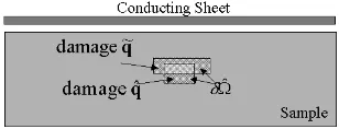
. We denote by4

-°

(see Figure 3) the points in

°

which are either in the damage represented by

or ¯

but which are not in both. In other words, let

°65

7 represent the points ´eµ¶f·d¹

in °

within the damage given by

and °

â

7 the points ´eµ¶·2¹

in °

within the damage given by ¯

. Then4 -°±&°5 798 ° â 7 ù°65 7;: ° â 7 .

Using the terminology above, we have the following theorem. Again, we refer the reader to [3, 8] for details and proof.

Theorem 2.2. Assume the admissible parameter set

¯

) Å+*

is a compact subset of » '

. Then there exists

± ´jöÆ¶øs¶ ¯ °¹

such that for source frequencies

ò ñ ´eö ¶øs¶ ¯ °Î¹ , ¯ ì´ ¯ ¹

is continuous from

¯

)ÖÅ,*

(6)

Figure 3: The Area Represented by<!=

>

3 Computational Method

To enable the techniques used in nondestructive evaluation to be implemented in a practical setting, we must not only locate and characterize subsurface damages; we need to do so in a fast and efficient manner. To develop a fast and efficient forward algorithm, we use the reduced order Karhunen-Loeve or Proper Orthogonal Decomposition (POD) methodology. A unique feature of the POD technique is its ability to create an ordered basis that models experimental or simulated data, capturing most of the important aspects of the data in the first few elements. Typically the number of basis elements required in the forward algorithm is reduced, resulting in the development of a faster algorithm that still maintains the accuracy of traditional finite element algorithms.

3.1 The POD Method

In this section we discuss the concepts and method of implementation of the POD method in the context of damage detection. For details on the general POD method, we refer the reader to [9, 10, 11, 12, 13, 14, 15, 16, 17, 18, 19, 20] and the extensive list of references contained therein. In the process of detecting a subsurface damage, a device, such as the GMR sensor, is scanned above (or below) a sample and data is taken. The variation in the field due to a damage is manifested in the data taken. Therefore, in forming a reduced basis, we want to incorporate the effects of a damage in the reduced basis. This is accomplished by taking “snapshots” of the data across various damages. In other words, let ? be a vector parameter

characterizing physical properties of the damage such as length, thickness, depth, etc. of the damage. Then given an ensemble of damages @A?CBEDAF!G

B+HJI , we obtain corresponding solutions,

@AKML3?CB NODAFPG

BQHJI , of the boundary

value problem, for magnetic vector potentials which we call our “snapshots”. We then use these snapshots to generate a basis incorporating the properties of the various damages. (Without loss of generality, we will denote the vectorK by its scalar nonzero componentR , i.e., theRTS component ofK .)

The formation of the POD basis can be summarized in a few steps. In order to successfully reduce the number of basis elements while maintaining accuracy, a single basis element must contain aspects of each damage?CB . Therefore, as explained in [20, 21], we seek basis elements of the form

UVXW F!G

Y

B+HJI[Z

V

L]\^N$R_L`?CB N (9)

where the coefficients

Z

V

La\bN are chosen such that each POD basis element

UV

,c

Wdfehg^ejiai]iae1k6l

, maximizes

d

k6l F!G

Y

B+HJI mon

R_L`?CB N

ehUVqp+rs1touwvx

y[z m{

(7)

subject to |~}O}+,C [a

}

. Forming the basis elements in such a way assures that a single basis element will contain information from each of the snapshots. From standard arguments, it can be seen that the coefficients C$]^ can be found by solving the eigenvalue problem 6

where is

given by

] 6^|3 _`¡Jh1 _`¡CQ "¢Oo£X [¤ (11)

Hence, the next step in forming the POD basis is to form the covariance matrix and find the

asso-ciated eigenvalues and eigenvectors. Since is Hermitian positive semi-definite, we know it possesses a

complete set of orthogonal eigenvectors and corresponding nonnegative eigenvalues. In forming the POD basis, we want to be able to readily decide which basis elements to use in the reduced basis. To this end, we order the eigenvalues along with their corresponding eigenvectors such that the eigenvalues are in decreasing order,

X¥§¦¨

¦ ¤]¤]¤ ¦¨ª©!«¦¬ ¤

(12)

We then normalize the eigenvectors corresponding to the rule

!P®A¯ ° ± ¤ (13)

Consequently, the²`³µ´ POD basis element is defined by Eq. (9) where!ab represents thef³µ´ component

of the² ³µ´ eigenvector of .

We now have the full POD basis and need a criterion to decide how many basis elements are re-quired to accurately portray the data. In other words, we want to choose

such that ¶Q·P¸º¹¼»"}3½

¥ . In choosing this number

, we compute

which represents the percentage of “energy” in ¶Q·P¸º¹¼»Á Â3¡Ch½

©

«

+¾

¥ that is captured in

¶1·!¸¯¹Å»"}ÆÁ½

©

+¾

¥ . Then

the reduced basis consists of the first

POD basis elements where

is chosen to capture the desired amount of energy.

We now note that ¶Q·P¸º¹¼»"}~½ ©!« µ¾ ¥ ¶Q·P¸º¹Å»Á _3¡ÇjO½ ©P« Q¾

¥ . Indeed, given any

Â3¡C, we have

_3¡Çj ©!« ÃÈ ¾ ¥ªÉ È `¡CQ} È (15) where É È `¡C |3 _`¡C h} È

¢ o£w Ê

(16)

as »"}Æ½ © «

Q¾

¥ are orthonormal in

Ë

`ÌÍhÎÏÐ .

However, to complete the analysis, one needs to be able to calculate

©

3¡[ where¡ is a given

param-eter not in the set »A¡Ç½ ©!«

+¾

¥ . To this end, we extend the approximation formula to obtain

(8)

where ÑÊÒºÓ`Ô[Õ can be evaluated through different methods. In [3], we explored two different methods

one might choose: a POD/Galerkin method or a POD/Interpolation method. However, in this paper, we only present results in which we use the POD/Interpolation method with linear interpolation for the one-parameter simulated results and cubic spline interpolation for all other results. For details on these meth-ods, we refer the reader to [22] and [23].

3.2 Simulated Results

In [4], we performed several trials in which we assumed we had access to various types of data, such as the Ö field or the × field at various points ÓØ!ÙÚ1ÛjÜ Õ in Ý . We compared and contrasted the accuracy to

which we could estimate the lengthÞ of the damage based on whether theÖ field or × field was used and

whether we considered the field along a single line, multiple lines or within the entire region (which is not experimentally possible and was only tested for initial comparisons). From the results presented in [4], we concluded that extremely accurate results were obtained only when the Û componentßáà of the magnetic

flux density was used in the cost criterion, i.e., when we used

â

Ó`Ô[Õäãåæèç

é

ÙµêJë

ì

é

ÜQêJë

í

åîï ßÂð

à

ÓqØ!Ù~Ú1ÛjÜÚOÔ[Õòñ

åîïó

ßáàÁÓØ!Ù~Ú1ÛEÜÚOÔwô1Õ

í

à

(18)

where

åî

ï

is a scaling factor accounting for the low order of magnitude of the field (ßáà is on the order

of

åîbõ

ïhöø÷ ù"ú

), ß

ð

Ó3Ô[ÕMã ûýüþÖ

ð

Ó3ÔwÕ is the reduced order POD approximation in which Ö

ð

Ó`Ô[Õ is

given by (17), and

ó

ßáà is “data” from a sample we wish to characterize. (In this section,

ó

ßáà is obtained

from Ansoft finite element simulations to which noise has been added in the usual manner (see [3, 21]). Furthermore, performing multi-line scans or using full region data improved the results only marginally and hence did not warrant the extra effort and time in collecting more extensive data sets. Consequently the results presented in this section involve only the least squares difference in the ßáà field given by (18)

along a single line located

å

úÿú

above the conducting sheet.

In the sample results presented, we focus on estimating a single parameter of the crack assuming all other parameters are fixed or estimating two parameters with one parameter fixed. The results below summarize the feasibility of determining the length and depth of a crack. In a specific trial run, ten different data sets (exact data with ten different sets of added random noise) are used where the relative noise is chosen at a

åî

noise level with a confidence level of (3 standard deviations). (Details can be found

in [3] and [4].)

In determining the length of the damage alone, we first followed the steps outlined in Section 3.1 and generated an ensemble of “snapshots”. Keeping the crack fixed at a depth of

úÿú

with a thickness of

æ

úÿú

, we varied the crack length Þ from

î

úÿú

to úÿú

in increments of

î

æ

úÿú

. Using the snapshots,

ÖÂÓ3ÞÜÕ ð êCàQë

Ü+êJë , we formed the POD basis and determined that

of the energy of the system was

cap-tured with a single basis element [4]. However, in the specific trial runs, we found that using POD basis

elements improved the parameter estimation with data containing no noise, while there was no significant difference between the use of basis elements over the use of basis elements. Therefore, the results are

based on the use of basis elements in the algorithm.

To test the inverse methodology, we first try to identify the length of the damage, Þ

ô

ã

å

úÿú

. Using data on a single line above the conducting sheet with

åî

relative noise, an average estimated length of

å

æ

úÿú

was obtained with a variance of

î

æ

Âü

åî õ

úÿú

à

(9)

Proceeding as we did in estimating the length of a damage, to estimate the depth of the damage, we fixed the thickness of the crack at with length and varied the depth of the crack from

to in increments of . Using 5 basis elements, we were able to accurately estimate

a crack depth of in the presence of! relative noise; an average depth of "#$ was estimated

with a variance #%$ '&(*),+-. . Thus, as in the case of estimating the length of a crack, we can also

recapture the depth of a crack quite accurately and efficiently.

Finally, we estimated both length and depth simultaneously. However, first, in [3, 8], we discussed in detail a need to modify the assumptions made in the original test problem to more accurately describe the behavior of experimental data used in the next section. In short, the computational domain was expanded beyond the edges of the sample and snapshots were taken of the magnetic flux density data on a single

line above the conducting sheet (instead of the whole region). Recall that for the previous trials, we took

snapshots of the magnetic vector potential for the entire computational domain even though in the inverse problem we only considered those data points along a single line. Furthermore, we considered data across the entire length of the sample, instead of just half the sample as done previously. (For more details , see [3, Chapter 6].) As a result, we also implement these changes in the two-parameter estimation problem.

We proceed as in the previous estimation problems by first generating an ensemble of damages. We consider damages with depths ranging from $ to $ in increments of in combination with

lengths from/ to"/ in increments of / (we now consider longer damages similar to those used

in obtaining experimental data). We keep the thickness fixed at$ . A total of 24 snapshots,01

.

2

354-6798: , ;=<

4$>%>4? , @

<

4$>%>4-A were generated using Ansoft. Using 4 basis elements with 10% relative noise

added, we estimated a damage with depth *B

<

A and length 6CB

<

/ . We obtained average

es-timates of

<

A with variance #,D&E*)*F?. and length 6

<

G /9 with variance

G"H&I,)*F?. . Thus, even when we estimated two parameters simultaneously, the computational

method proposed produced extremely accurate results.

3.3 Experimental Results

Since the results using simulated data were extremely promising, we designed an experiment in which we tried to detect and parameterize a damage within an aluminum sample using a giant magnetoresistive (GMR) sensor. The sample was constructed of 17 layers of $ thick aluminum plates with a slice cut

out of one of the layers to simulate a damage within the sample (see [3, 8] for graphical representations). The “damaged” piece of aluminum is moved from one layer to another to simulate damages within the sample at different depths, and the length of the damage is varied by producing “gaps” of varying size from the aluminum plate (the thickness of the damage is always fixed at J ). As a means of inducing

current within the sample, a thin sheet of copper carrying a uniform current of " Amps is placed above

the sample on top of a thin sheet of paper (to avoid direct physical contact between the sample and the conducting sheet). The GMR sensor measures the amplitude and phase of the magnetic flux density across a

;LK

line (along the length of the sample) every " . The data is then filtered through a lock-in

amplifier and saved to a file.

(10)

given by

MONQPSRUTWV

X

YCZ\[

]

^`_\a?b [

c

cVde?f=g

[

NCh

^ji PkRml

Vdeonf

^

[

c

[qp

(19)

where

P

is the vector containing the parameters we wish to estimate, f

g

[

NQPkR

is the POD approximation formed using snapshots on the data itself,fsrn

[ is GMR data at grid points

h

^

, t

T

V

p$u>u>u%p-v

with

v

total grid points andw andx indicate the indices of the grid points we consider in our cost criterion.

In estimating a depth of y,z

T|{}}

with corresponding length ~Cz

T

V

u

}

, we obtained an estimate of y

T

X

u

}}

and ~

T

V

u

V

X

}

, resulting in a relative error for depth of

T

d

u

d and length

T X u

. Again, even with experimental data, the results were accurate.

4 Conclusion

In this paper we presented a reduced order computational algorithm which contributes to the overall field of nondestructive evaluation. In detecting subsurface damages, there is a need for a fast and efficient inverse problem methodology. The reduced order POD method is an attractive method, because it allowed us to create a reduced basis of less than 10 basis elements in the trials presented while still capturing 99% of the total energy of the system. This results in an accurate, as well as fast, forward algorithm.

We then gave an overview of the POD methodology in the context of subsurface damage detection or parameter identification. We discussed the implementation of the inverse problem for both simulated results as well as experimental results, providing examples for each case. Based upon the results presented, we showed that using either simulated data or experimental data on either a one-parameter estimation problem or a two-parameter estimation problem, we achieved accurate results.

However, the most significant finding is in regard to reduction in computational time which can be sum-marized as follows. If one were to use a software package such as Ansoft’s Maxwell 2D Field Simulator to calculate the forward problem each time it is required in the inverse problem, it would take approximately 5-10 minutes for a single forward solve. The forward solve is typically required anywhere from as few as 10 times to as many as 500-1000 times. Assuming the forward algorithm is called approximately 100 times with an average of 7 minutes for each forward run, the inverse problem would take approximately 42,000 seconds. In the examples provided, the entire inverse problem ran in approximately 8-10 seconds. Consequently, on average the computational time is reduced by a factor of V$d . This suggests that an

ap-propriate sensing device, when coupled with reduced order modeling in the inverse problem, might prove feasible in practical damage detection applications.

Acknowledgments

(11)

References

[1] Buzz Wincheski and Min Namkung. Development of very low frequency self-nulling probe for inspection of thick layered aluminum structures. In 1998 Review of Progress in Quantitative NDE, Snowbird, Utah, Aug. 1998.

[2] Buzz Wincheski and Min Namkung. Deep flaw detection with giant magnetoresistive (GMR) based self-nulling probe. In 1999 Review of Progress in Quantitative NDE, Montreal, Canada, July 1999.

[3] Michele L. Joyner. An Application of a Reduced Order Computational Methodology for Eddy Current Based

Nondestruc-tive Evaluation Techniques. PhD thesis, North Carolina State University, 2001.

[4] H.T. Banks, M.L. Joyner, B. Wincheski, and W.P. Winfree. Evaluation of material integrity using reduced order compu-tational methodology. CRSC Tech. Rep. CRSC-TR99-30, North Carolina State University, 1999.

[5] David K. Cheng. Field and Wave Electromagnetics. Addison-Wesley, Reading, MA, second edition, 1992.

[6] Ansoft Corporation. Maxwell 2D Field Simulator - Technical Notes, 1995-1999.

[7] Lawrence C. Evans. Partial Differential Equations. American Mathematical Society, Providence, 1991.

[8] H.T. Banks, M.L. Joyner, B. Wincheski, and W.P. Winfree. Real time computational algorithms for eddy current bas based damage detection. In progress.

[9] H.T. Banks, R.C. del Rosario, and R.C. Smith. Reduced order model feedback control design: Numerical implementation in a thin shell model. IEEE Trans. Auto. Control, 45:1312–1324, July 2000.

[10] G. Berkooz. Observations on the proper orthogonal decomposition. In Studies in Turbulence, pages 229–247. Springer-Verlag, New York, 1992.

[11] G. Berkooz, P. Holmes, and J.L. Lumley. The proper orthogonal decomposition in the analysis of turbulent flows. Annual

Review of Fluid Mechanics, 25(5):539–575, 1993.

[12] R.C. del Rosario. Computational Methods for Feedback Control in Structural Systems. PhD thesis, North Carolina State University, 1998.

[13] K. Karhunen. Zur spektral theorie stochasticher prozesse. Ann. Acad. Sci. Fennicae, 37(A1), 1946.

[14] M. Kirby and L. Sirovich. Application of the Karhunen-Loeve procedure for the characterization of human faces. IEEE

Transactions on Pattern Analysis and Machine Intelligence, 12(1):103–108, 1990.

[15] M. Kirby, J.P. Boris, and L. Sirovich. A proper orthogonal decomposition of a simulated supersonic shear layer.

Interna-tional Journal for Numerical Methods in Fluids, 10:411–428, 1990.

[16] K. Kunisch and S. Volkwein. Control of Burgers’ equation by a reduced-order approach using proper orthogonal decom-position. J. Optimization Theory and Applic., 102(2):345–371, 1999.

[17] M. Loeve. Functions aleatoire de second ordre. Compte rend. Acad. Sci., Paris, 1945.

[18] J.L. Lumley. The structure of inhomogeneous turbulent flows. Atmospheric Turbulence and Radio Wave Propagation, pages 166–178, 1967.

[19] J.L. Lumley. Stochastic Tools in Turbulence. Academic Press, New York, 1970.

[20] H.V. Ly and H.T. Tran. Proper orthogonal decomposition for flow calculations and optimal control in a horizontal cvd reactor. CRSC Tech. Rep. CRSC-TR98-13, North Carolina State University, 1998, Quart. Appl. Math, to appear.

[21] H.T. Banks, M.L. Joyner, B. Wincheski, and W.P. Winfree. Nondestructive evaluation using a reduced-order computational methodology. Inverse Problems, 16, 2000.

[22] Alfio Quarteroni, Riccardo Sacco, and Fausto Saleri. Numerical Mathematics. Springer-Verlag, New York, 2000.