ABSTRACT
KULAHLIOGLU, ADEM HALIL. Applications of the Fixed-Node Quantum Monte Carlo Method. (Under the direction of Lubos Mitas.)
Quantum Monte Carlo (QMC) is a highly sophisticated quantum many-body method. Dif-fusion Monte Carlo (DMC), a projected QMC method, is a stochastic solution of the stationary
Schr¨odinger’s equation. It is, in principle, an exact method. However, in dealing with fermions,
since trial wave functions meet the antisymmetric condition of the many-body fermionic sys-tems, it inevitably encounters the fermion sign problem. One of the ways to circumvent the sign
problem is by imposing the so-called fixed-node approximation.
The fixed-node DMC (FN-DMC), a highly promising method, is emerging as the method of choice for correlated treatment of many-body electronic structure problems since it is much
more accurate than Khon-Sham DFT and has a competitive accuracy with CCSD(T) but scales
better with system size than CCSD(T).
An important drawback in FN-DMC is the fixed-node bias introduced by the approximate
nature of the trial wave function nodes. In this dissertation, we examine the fixed-node bias
and its restrictive impact on the accuracy of FN-DMC. Also, electron density dependence of the fixed-node bias is discussed by taking a relatively small atomic system.
In our dissertation, we also applied FN-DMC in a relatively large molecular system with
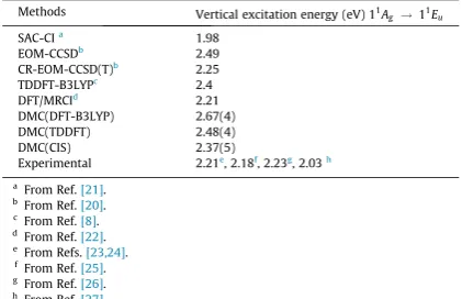
a transition metal, Zinc-porphyrin, to calculate the excitation energy in an adiabatic limit (vertical excitation). We found that FN-DMC results agree well with experimental values as
well as with results obtained by some other correlated ab initio methods such as CCSD.
In addition, we used FN-DMC to study a transition metal dimer, Mo2, which is a challenging system for theoretical studies since there is large amount of many-body correlation effects. We
constructed the antisymmetric part (Slater part) of the trial wave function by means of the
Selected-CI method. Moreover, we carried out CCSD(T) calculations in order to be able to compare FN-DMC energies with another correlated method energies. FN-DMC and CCSD(T)
calculations in Mo2, which is dominant with d-d bondings, enabled us to make comparisons
©Copyright 2014 by Adem Halil Kulahlioglu
Applications of the Fixed-Node Quantum Monte Carlo Method
by
Adem Halil Kulahlioglu
A dissertation submitted to the Graduate Faculty of North Carolina State University
in partial fulfillment of the requirements for the Degree of
Doctor of Philosophy
Physics
Raleigh, North Carolina
2014
APPROVED BY:
Chueng Ji Christopher Roland
Alper Bozkurt Lubos Mitas
DEDICATION
To my dear wife, To my dad,
To my mom, To my sisters,
To my relatives who really care me with their prayers,
To my teachers,
To my friends who were always supportive to me,
To anybody who touched ever my life positively, even with a single word or with a single glass
BIOGRAPHY
”Science is to perceive the reality of science, Science consists in knowledge of the self;
If, then, you do not know your self,
I wonder what kind of education you have had.” –Yunus Emre (a Turkish poet,
1240-1320)
ACKNOWLEDGEMENTS
I would like to thank my advisor, Dr. Lubos Mitas, for his help. Probably I couldn’t complete my doctorate study without his academic support. His enthusiasm and critical thinking were always
inspiring for me. I was very often impressed by his deep knowledge and crystal clear memory. Of course, his patience towards us during the progress of the projects was the top favor that I
appreciated the most. Probably I will never forget his advice that the background information
of the method should be reviewed several times so that it becomes the second nature. I am very proud that I was one of his doctorate students. The time I spent by co-working with him under
his guidance is, I believe, an invaluable experience for my academic life.
I am also very thankful to Dr. Chueng Ji, Dr. Christopher Roland, and Dr. Alper Bozkurt for being a member in my committee and for their precious time. They always welcomed my
requests to cooperate in the processes of the preliminary and final exams and also in many
other issues.
I will always remember the favors that I received from my research group fellows. Without
their help many things would be great headaches for me.
I can not conclude this page without acknowledging the positive contributions of my former advisor Dr. Kasif Sabeeh in my academic career. He has not only provided an academic
mentor-ship but also approached me very friendly. He often spared his precious time to me generously.
I would like to thank him, as well.
Also I would like to express a speacial thank to Dr. Kenan Gundogdu for his academic
advices and the discussions we had together.
And I would also like to thank the department of Physics (my department), especially to Prof. Harald Ade and Prof. Chueng Ji for being the director of graduate programs.
I express my thanks to all the professors those who taught me and all the administrative
stuff of our department, especially Rhonda Bennett, Leslie Cochran, Chastity Buehring and Rebecca Savage, who helped us to have an easy life in the department.
I would like to express my most special thanks to my wife who shared all happy and hard
times that I had during my doctorate study and to my parents who were self-sacrificing for their children.
And I am thankful to many persons and many friends that I can not name here. For instance, having friends such as Murat An (phys. dep.), Fahri Sarac (MSE) and Ismail Demir (math dep.)
TABLE OF CONTENTS
LIST OF TABLES . . . vii
LIST OF FIGURES . . . .viii
Chapter 1 Introduction . . . 1
Chapter 2 Some Conventional Electronic Structure Methods . . . 5
2.1 Born-Oppenheimer Approximation . . . 6
2.2 Many-electron systems and independent-electron approximation . . . 8
2.3 The Hartree-Fock Method . . . 9
2.3.1 The Variational Principle . . . 11
2.3.2 SCF with a basis set: The Roothan Equations . . . 12
2.3.3 Basis Functions Types . . . 14
2.4 Configuration Interaction (CI) Method: As a Post-HF method . . . 15
2.4.1 Excited Determinants and CI expansion . . . 16
2.4.2 Full CI and Complete Basis Set (CBS) Limit . . . 16
2.4.3 Truncated CI . . . 17
2.4.4 Configuration State Functions (CSFs) . . . 19
2.5 Density Functional Method (DFT) . . . 20
2.5.1 Thomas-Fermi (TF) Approximation . . . 21
2.5.2 The Hohenberg-Khon Theorems . . . 22
2.5.3 The Khon-Sham Approach . . . 24
2.6 Pseudopotentials (PP) . . . 27
Chapter 3 Quantum Monte Carlo Methods . . . 30
3.1 Monte Carlo Integration . . . 30
3.1.1 Random Numbers . . . 31
3.1.2 Sampling . . . 32
3.1.3 Importance Sampling . . . 32
3.1.4 The Central Limit Theorem . . . 33
3.1.5 Random Walks and Markow Chains . . . 34
3.1.6 Metropolis Algorithm . . . 34
3.1.7 Sampling|Ψ(R)|2 . . . 36
3.2 Variational Monte Carlo (VMC) Method . . . 38
3.3 Diffusion Monte Carlo (DMC) Method . . . 40
3.3.1 Introduction: A projection method . . . 40
3.3.2 Green’s Function . . . 42
3.3.3 DMC with Importance Sampling . . . 44
3.3.4 Improved Green’s Function . . . 46
3.3.5 Fermion Sign Problem and Fixed-Node Approximation . . . 46
3.3.6 The Tiling Theorem and Variational Fixed-Node DMC . . . 47
3.3.7 The Mixed Estimator and Reptation Quantum Monte Carlo . . . 49
3.3.9 PseudoPotentials and QMC: Locality Approximation and T-Moves . . . 51
3.4 Trial Wave Functions . . . 52
3.4.1 Antisymmetric Wave Functions (The Slater Part) . . . 53
3.4.2 Jastrow Function . . . 57
3.4.3 Cusp Conditions . . . 59
3.4.4 Wave Function Optimization . . . 61
Chapter 4 Preface to Results . . . 66
Chapter 5 Density dependence of fixed-node errors in diffusion quantum monte Carlo: Triplet pair correlations . . . 67
Chapter 6 A quantum Monte Carlo study of zinc-porphyrin: Vertical excita-tion between the singlet ground state and the lowest-lying singlet excited state . . . 73
Chapter 7 A QMC Study of Mo2 . . . 78
7.1 Selected-CI method . . . 80
7.2 Computational Details . . . 82
7.3 Results and Discussion . . . 84
7.4 Conclusion . . . 92
LIST OF TABLES
Table 3.1 Some functions commonly used in the Jastrow correlation terms [6]. . . 58
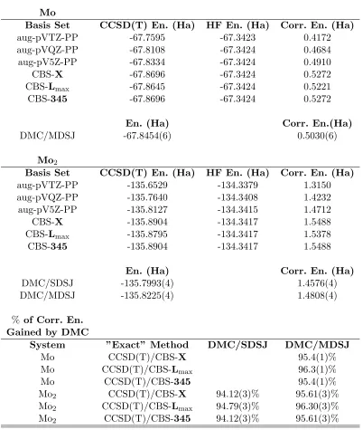
Table 7.1 The CCSD(T) and DMC energies of Mo and Mo2 and the percentages of
the correlation energies recovered by DMC are given. Note that the ener-gies are given only for the purpose of comparison between the CCSD(T) and DMC methods, otherwise, the energies are specific to the pseudopotentials employed in the calculations. The CBS extrapolation methods denoted as CBS-X, CBS-Lmax and CBS-345 are explained in the text and also given in Eqs. (7.9),(7.10) and (7.11), respectively. DMC/SDSJ and DMC/MDSJ stand for DMC calculations with single-determinant and multi-determinant trial wave functions, respectively. Note that the difference between the DMC/SDSJ and DMC/MDSJ energies in the atomic state (Mo) was actually negligible. . . 86
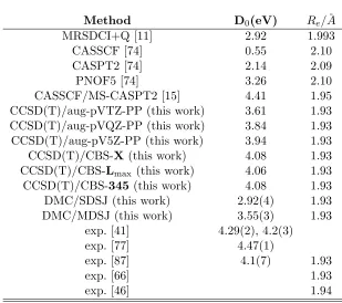
Table 7.2 The binding energies of Mo2 obtained by several methods are given. The
LIST OF FIGURES
Figure 3.1 A square of width 2R and a circle of radius R are shown. The points are
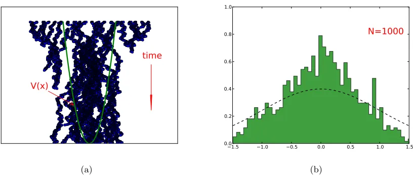
randomly drawn. The red points are inside the circle, however, the others are outside of the circle. The ratio of the red points to the total number of points is equal to the ratio of the area of the circle to that of the square (in the limit that the number of points goes to the infinity). . . 31 Figure 3.2 An instructive demonstration of the birth/death algorithm is given. The
sam-pling of the ground state of a single-particle system under the harmonic po-tential is depicted. In Fig (a), the walkers are uniformly distributed at the initial time. As time elapses, the walkers undergo the annihilation/branching process. The readjustment of the walker population is in the favor of the low potential points. In Fig (b), the redistribution of the walkers samples the ground state of the system. It is given that the number of the walkers is 1000. The dashed line shows the exact ground state. . . 44
Figure 7.1 Mo2 energy obtained by the DMC and VMC methods with varying number
of determinants are given. The estimated exact energy is based on the as-sumption that the DMC energy of Mo is exact and calculated by considering the experimental binding energy value, 4.29(2) eV and an estimated value of the zero-point-energy, 0.03 eV. The percentages correspond to the percent-ages of the correlation energies gained by DMC/SDSJ (DMC with a single-determinant Slater-Jastrow type wave function) and DMC/MDSJ(DMC with a multi-determinant Slater-Jastrow type wave function). Error bars for the
VMC and DMC energies are much smaller than the scale of the graph. . . . 89
Figure 7.2 The CBS extrapolation of the HF energies of Mo obtained with the basis sets aug-pVXZ-PP is shown. The formula given in Eq. (7.13) is exploited as the extrapolation scheme. . . 90
Figure 7.3 The CBS extrapolations of the correlation energies of Mo obtained by the
CCSD(T)aug-pVXZ-PP method are shown. The formulas given in Eqs. (7.9), (7.10) and (7.11) are exploited as the extrapolation schemes denoted as CBS-X, CBS-Lmax and CBS-345, respectively. CBS-X and CBS-345 yield almost identical correlation energies, however, CBS-Lmaxresults in a slightly lower correlation energy. . . 90
Figure 7.4 The CBS extrapolation of the HF energies of Mo2 obtained with the basis
sets aug-pVXZ-PP is shown. The formula given in Eq. (7.13) is exploited as the extrapolation scheme. . . 91 Figure 7.5 The CBS extrapolations of the correlation energies of Mo2 obtained by the
CCSD(T)aug-pVXZ-PP method are shown. The formulas given in Eqs. (7.9), (7.10) and (7.11) are exploited as the extrapolation schemes denoted as CBS−
Chapter 1
Introduction
”Science never solves a problem without creating ten more,” says B. Shaw [17]. This is so true that we observe this pattern in every aspect of the science. Rutherford solved one problem by
demonstrating a nuclear atom which would lead to that an atom is made up a positive nucleus
and a number of negative electrons [4]. However, this theorem led to a planetary system-like visualization of an atom, which conflicted with the electromagnetic theory; a radiating particle
should decay eventually [49]. In later years, this conflict was lifted by the emergence of quantum
physics, which could describe states where electrons are stable with certain discrete energy values in an atom [65].
Quantum physics presents to us consistent and accurate pictures of systems and it is
nowa-days seen more reliable than the classical physics in investigating the properties of materials. This is especially true when small-scale physics is important in those properties. However, it is
rarely the case that we find a solvable quantum system - even though it is nicely formulated
by quantum physics- without making a number of approximations. This is the reason I found B. Shaw’s wry aphorism very meaningful. On the one hand, quantum mechanics offers a valid
and reliable stream of comprehension of the materials, on the other hand, it forms a chain of
”problems” which arise from the lack of our technical ability to carry out the calculations that quantum mechanics leads us to . This fact was stated perhaps the most famously by Dirac
regarding Dirac’s equation [28]:
”The underlying physical laws necessary for the mathematical theory of a large part
of physics and the whole chemistry are thus completely known, the difficulty is only that the exact application of these laws leads to equations much too complicated to
be solvable”.
Likewise, Feynman concludes his speech ”Simulating physics with computers” [33], with the
”I’m not happy with all the analyses that go with just the classical theory, because
nature isn’t classical, and if you want to make a simulation of nature, you’d better make it quantum mechanical, and by golly it’s a wonderful problem, because it
doesn’t look so easy.”
If we confine ourselves to the electronic structure calculations (a framework of molecular
and condensed matter quantum systems), the most outstanding challenge is perhaps when the difficulty in dealing with the physical problems in the framework of quantum physics (such
as the wave behavior, discrete allowed levels) is multiplied by the complexity of the relations
(equations) originated from the many-body interactions. These interactions couple the indi-vidual quantum particles states with each other. Hence, as the number of quantum particles
increases, the resulting mathematical system of equations becomes increasingly complicated. In
fact, any many-body quantum problem is insolvable analytically; a two-body problem can be reduced to a one-body problem [71].
For simplicity, if we ignore the relativistic effects, the electronic structure of a quantum
system (atoms, molecules and periodic systems) is governed by the stationary Schr¨odinger’s many-body equation:
HΨ(X) =EΨ(X) (1.1a)
H=X
I
PI2 2mI
+X
i
Pi2 2me
+X
i<j 1 rij
+X
iI
−ZI
riI
+V(X) +X I<J
ZIZJ
RIJ
(1.1b)
wherei,jandI,J are electrons and nuclei indices, respectively1.mIandmeare the nucleus and electron masses, respectively. X is the generalized coordinates (i.e. positions and spin states).
rij, riI and RIJ are the electron-electron, electron-nucleus and nucleus-nucleus distances. In
practice, this complex equation can not be solved without making a number of approximations. The first and most obvious approximation is perhaps the decoupling of the nuclei terms
from the electronic ones (i.e., Born-Oppenhemier approximation) [79].
After putting the relatively ”heavy” nuclei terms aside, we now have to deal with only electrons. However, even this simplified form of the Schr¨odinger’s equation is far from practical
solvability (again except in very small systems).
The first attempt to overcome this well-known difficulty of the Schr¨odinger’s equation was by the Hartree-Fock (HF) method. Although this method is now seen quite primitive, it is
the starting point of many other more sophisticated methods in their formality; they originate
from the HF method. The HF method approximates the solution by transforming the explicit electron-electron interaction into a mean-field problem [56, 79]. Hence, although the HF method
1
provides a lot of information about a system, it misses the information originating from the
electron-electron interaction (later on we will call this missing piece as the correlation). Many methods have been developed to recover the correlation energy. These include the post-HF
methods, which can be seen the derivatives of the HF method [79].
In addition to the post-HF methods, The Density Function Theory (DFT) method was developed to recover the electron-electron correlation. DFT also originates from the formalism
of the HF method (hence, it is also an iterative mean-field method) but now the electron-electron
interaction is explicitly taken care of in the form of density functionals [56].
The Post-HF and DFT methods with their advantages and limitations have been widely
used for many decades. The post-HF methods, for instance CCSD(T) and CI, are very accurate
but they have very poor scaling with system size. However, DFT is computationally cheap and mostly provides satisfactory results; that is the reason it is a highly popular technique. The
disadvantage of DFT is that its accuracy is biased by the empirical choice and approximate
form of the density functionals (i.e., the exact functionals are not known yet) [6, 55, 35]. These examples show that considering the reliability and applicability of a method in
elec-tronic structure calculations, there is space for a method offering both of them. The Quantum
Monte Carlo (QMC) method is an emerging promising method in this context. It provides highly accurate results (even such that DFT functional LDA has been fitted by using the QMC
num-bers in homegenous electron gas [23]) and has much better scaling than the above-mentioned post-HF methods.
In this dissertation, the QMC approach in the electronic structure theory will be discussed.
Among many QMC methods, only the methods which are relevant to our work –namely Dif-fusion Quantum Monte Carlo (DMC) and Variational Monte Carlo (VMC) methods– will be
considered. In fact, since VMC is usually a preliminary tool for a DMC calculation –i.e. it can
be used as a framework in wave function optimization priori a more sophisticated method, DMC –, the focus will be on DMC and its applications.
As we already noted, quantum systems are difficult to simulate. Among the most immediate
examples of this statement is the well-known fermion sign problem. By confining ourselves to the electronic structure calculations, we deal with fermions and due to the specific sign symmetry of
fermionic wave functions, we inevitably encounter a fundamental formal problem in DMC; the
original formalism becomes impractically inefficient for fermions. There are a few prescriptions for this problem. However, perhaps the most practical and widely used one is the fixed-node
approximation [73, 6, 35]. So the fixed-node DMC will be our primary concern.
The organization of this dissertation will be as follows: In chapter 2, we will briefly discuss the ”conventional” electronic structure methods: HF, post-HF and DFT methods. In chapter 3,
QMC methods (VMC and DMC) will be introduced. In chapter 5, we will present an analysis
this point, we will discuss the relation between the fixed-node bias and the electron density. This
endeavor to comprehend the fixed-node bias will be in the frame of a 3-electron atomic system. In chapter 6 an application of the fixed-node DMC to a relatively large molecular system,
zinc-porphyrin, will be presented. We will discuss how we employed QMC in the investigation of a
spectroscopic property of the molecule. More specifically, a vertical excitation energy calculation which is associated with the Q band will be discussed. Chapter 7 covers our attempt to calculate
the binding energy of Molybdenum dimer, Mo2, in a variational approach which is original to
Chapter 2
Some Conventional Electronic
Structure Methods
Electronic structure theory aims to provide an understanding and description of a rich spectrum
of phenomena that we observe in materials, quantitatively [56].
The properties of the materials can be classified as those associated with the ground state and excited states. For instance, the properties which are determined mostly by the ground state
are cohesive/binding energy, equilibrium geometry of crystals, elastic behaviors, some dielectric and magnetic properties etc.. On the other hand, specific heat, transport, insulating gaps and
optical properties are some properties which excited states describe effectively [56].
Description and analysis of these properties require dealing with the quantum many-body problem. This many-body problem involves electrons, nuclei (ions) and their coupling with each
other.
For brevity, we can choose to exclude the relativistic effects. Then a quantum system that we are considering in the context of electronic structure theory is governed by the stationary
Schr¨odinger’s equation. The non-relativistic Hamiltonian given in Eq. (1.1) can be rewritten as
follows:
H=X
I
− ∇
2 I 2mI
+X
i
−∇
2 i 2mi
+X
i<j 1 rij
+X
iI
−ZI
riI
+X
I<J
ZIZJ
RIJ
+ ˆVext (2.1)
where i, j are the electron indices, I, J are the nuclei indices, mi, mI are the electron and
nucleus masses respectively. r and R denote the electron and nucleus positions, respectively. rij,riI and RIJ are the relevant interparticle distances. ˆVext is the external potential operator.
H = ˆTn+ ˆTe+ ˆVee+ ˆVen+ ˆVnn+ ˆVext (2.2)
where the terms denote the nuclear kinetic energy, electronic kinetic energy, electron-electron
interaction, electron-nucleus interaction, nucleus-nucleus interaction and finally the external potential. It follows that the Schr¨odinger’s equation is given by:
HΨ(r,R) =EΨ(r,R) (2.3)
where Ψ(r,R) is the many-body combined wave function of the electrons and nuclei. This
equation would be much simpler if the electron-nucleus interaction ( ˆVen) was non-existing,
since it results in the coupling of the electron motion with the nuclear motion. However, it is
usually not small enough to be neglected.
2.1
Born-Oppenheimer Approximation
We seek a valid simplification on Eq. (2.3). That is what the BornOppenheimer approximation (BOA) [16, 48] actually meant. It decouples the electron motion from the nuclear motion. In
order to reach the simplification thatBOA yields, let us write the hamiltonian given in Eq 2.2
as follows:
H =Hn+He (2.4)
Hn= ˆTn (2.5)
He= ˆTe+ ˆVee+ ˆVen+ ˆVnn+ ˆVext (2.6)
Furthermore, let us assume that the wave function in Eq 2.3 can be recast into a product of electronic and nuclear wave functions in which the former will depend on r and R while the
latter will be dependent on onlyR as follows:
Ψ(r,R) = Φ(r,R)χ(R) (2.7)
where Φ(r,R) andχ(R) are the electronic and nuclear wave functions, respectively. Then, the
nuclear part of the Schr¨odinger’s equation given in Eq. (2.3) becomes as follows:
HnΨ(r,R) =−
1 2
X
I 1
mI
[Φ(r,R)∇2Iχ(R) +χ(R)∇2IΦ(r,R)
Please note that∇I is in terms of the nuclear positionRI. The third term on right hand side of Eq. (2.8) will vanish. This can be justified if the term is multiplied by Φ(r,R)∗ and integrated overrspace, then it will be proportional to the following :
∇I
Z
dr|Φ(r,R)|2 =∇
I(1) (2.9)
=0 (2.10)
where the integral yields the normalization which is independent of R. For the second term,
∇IΦ(r,R) is in the same order of magnitude as∇iΦ(r,R), where please recall that∇i acts with respect to the electron position. This can intuitively be seen as both of ∇i and ∇I act in the same dimensions. Since∇IΦ(r,R)∼ ∇iΦ(r,R) =ipeΦ(r,R) –wherepeis electron momentum– , the second term on right hand side of Eq. (2.8) will give p2e
2mI which is proportional to
mi
mI, the ratio of the electron mass to the nuclear mass. Roughly speaking, since this ratio is small
enough, we can drop the second term. Thus, it follows that
HnΨ(r,R)≈Φ(r,R)Hnχ(R). (2.11)
Following from the Eqs. (2.11) and (2.4), the Schr¨odinger’s equation given in 2.3 becomes as
follows:
Hnχ(R)
χ(R) +
HeΦ(r,R)
Φ(r,R) =E (2.12)
where we can choose Φ(r,R) such that it obeys the following equation:
HeΦk(r,R) =εk(R)Φk(r,R) (2.13)
where the subscripts inεk and Φkare introduced in order to show that there are various states; i.e., the BO surfaces. Also it is noteworthy thatRnuclei positions exist inεk(R) as a parameter.
If we substitute 2.13 into 2.12, then we will have the following:
[Hn+εk(R)]χ(R) =Eχ(R). (2.14)
The BO approximation holds as long as the surfaces, εk(R), are well separated such that
|εk−1(R)| εk(R). (2.15)
Otherwise, the second term on right hand side of Eq. (2.8) will no longer be negligible.
The BO approximation is a two-step process. In the first step, the electronic part of the wave
are present in the electronic wave function as parameters. In the second step, by knowing the
contribution of the electronic motion in the nuclear motion, which is meant by substituting εk(R) into Eq. (2.15), the nuclear motion is described.
This approximation rests on the assumption that electrons immediately reach their ground
state upon motion of nuclei, zero relaxation time. In most cases, the BO approximation is a good approximation and simplifies the Schr¨odinger’s many-body problem given in Eq. (2.3)
drastically. In the rest of this dissertation, we will rely on the BO approximation and investigate
only the electronic part of the hamiltonian, i.e. He given in Eq. (2.4) which is based on fixed nuclei positions.
2.2
Many-electron systems and independent-electron
approxi-mation
The Schr¨odinger’s equation, even after the BO approximation, is still prohibitively difficult.
The difficulty stems from that the fact that electrons (ions are considered to be still at their equilibrium points in the BO approximation) interact with each other and this makes their
motions coupled with each other. Thus, in principle, the exact wave function (i.e., the solution
of the Schr¨odinger’s equation) must be a many-body wave function which incorporates the
electron-electron interaction.
One of the approaches towards the problem is to substitute the complicated electron-electron
interactions with an average potential felt by each electron individually; this potential is called the mean-field. This approach is known as the mean-field theory. This substitution will
natu-rally transform the many-body problem into an independent-electron system under an effective
hamiltion defined with the mean field.
The independent-electron approaches can fall into two general categories: thenon-interacting
and Hartree-Fock methods [56]. The point where they differ is that while the HF method
in-cludes the electron-electron interaction explicitly, the non-interacting method does not. How-ever, both approaches are still in the framework of the independent-electron approximation
and thus fail to describe the exact electron-electron correlations which exist in the true wave
function. In the non-interacting theories, instead of explicit electron-electron interaction terms, there is an effective potential which is defined in terms of some parameters.
The non-interacting approach is often named as Hartree or Hartree-like since D. R. Hartree was the first one who used this approach. The Khon-Sham approach in DFT is counted in this
class by acknowledging the fact that the Khon-Sham effective potential (which is in terms of
The non-interacting (Hartree-like) approximation leads to the following eigenvalue equation
ˆ
Heffψiσ(r) = (− 1 2∇
2+vσ
eff(r))ψσi(r) =εiψiσ(r) (2.16)
wherevσeff(r) is the effective potential felt by an electron atrwith the spinσ. The most crucial question here is how to build vσ
eff(r) so that it will mimic the exact many-body potential. In Hartree’s original work, effective potential was poorly defined. In the modern Khon-Sham DFT
method, it is constructed as a density functional, i.e., a function of electron density.
It is worthwhile to note that Eq. (2.16) leads to orthogonal orbits (single-electron wave
functions) which in turn can be used to form an antisymmetric wave function, referred to as
the Slater determinant (see Sec. (2.3)).
2.3
The Hartree-Fock Method
The Hartree-Fock (HF) method is important not only because it has a special place in the history
of Quantum Chemistry (electronic structure theory) but also because it is a starting point for many modern, more accurate, correlated methods. Some methods involve improvements
upon the HF wave function such as Configuration Interaction (CI) and Coupled Cluster (CC) methods. Some other methods simply use the results of HF calculations; for instance QMC uses
the HF wave function as a trial wave function. Therefore, the HF method has a unique place
in electronic structure methods [56, 79].
For simplicity, let us assume that the exact hamiltonian does not contain sporbit
in-teraction, magnetic field and relativistic effects. And let the single-electron ”spin orbitals” be
ψσj
i (rj) = ψi(xj) which is the product of spatial and spin functions, i.e., ψi(xj) = φi(rj)χi(σj) where we introduced the general coordinate, xj = (rj, σj). We now consider a system of N
electrons. For easy notation, let X and R be the many-body general and spatial and spin
co-ordinates while xi, ri and σi be the general, spatial and spin coordinates of the ith electron. Thus, it follows that
X= (x1,x2, ...,xN)
R= (r1,r2, ...,rN)
Due to the indistinguishablity symmetry of electrons, an electronic many-body wave function carries the anti-symmetry which is that the wave function changes sign upon an interchange
anti-symmetry requires that
Φ(x1,x2, ...xi, ...xj, ...,xN) =−Φ(x1,x2, ...xj, ...xi, ...,xN) for i, j= 1, ...N. (2.17)
The simplest form of an anti-symmetric many-body fermion wave function generated out of
single-particle orbitals,ψi(xj) is perhaps a Slater determinant
Φ(X) = 1
(N!)1/2
ψ1(x1) ψ1(x2) ... ψ1(xN)
ψ2(x1) ψ2(x2) ... ψ2(xN)
... ... ... ...
ψN(x1) ψN(x2) ... ψN(xN)
(2.18)
which will be denoted, throughout this dissertation as|ψ1(x1)ψ1(x2)...ψ1(xN)i.
We can recast the electronic hamiltonian given in Eq. (2.4) within the BO approximation
as follows:
H =X
i ˆ
hi+
X
i<j 1 rij
+Vnn (2.19)
ˆ
hi =−
1 2∇ 2 i − X I ZI
|riI|
+Vext(xi) (2.20)
Vnn =
X
I<J
ZIZJ
|RIJ|
(2.21)
The energy estimation with the Slater determinant given in Eq. (2.18) will be
E=hΦ(x)|H|Φ(x)i= N
X
i
Z
dr1φ∗i(r1)ˆh1φi(r1)+
1 2 N X i,j Z
dr1dr2φ∗i(r1)φ∗j(r2) 1 r12
φi(r1)φj(r2)+
−1 2 N X i,j Z
dr1dr2φ∗i(r1)φ∗j(r2) 1 r12
φj(r1)φi(r2)δσi,σj+Vnn (2.22)
where the spatial orbitals take place explicitly. The preceding equation can be rewritten in a compact form as follows:
E=
N
X
i
Hii+
1 2
N
X
ij
where
Hii=
Z
dr1φ∗i(r1)ˆh1φi(r1) (2.24)
Jij = Z
dr1dr2φ∗i(r1)φ∗j(r2) 1 r12
φi(r1)φj(r2) (2.25)
Kij =
Z
dr1dr2φ∗i(r1)φ∗j(r2) 1 r12
φj(r1)φi(r2)δσi,σj. (2.26)
Jij and Kij are called Coulomb integrals and exchange integrals, respectively.
In a restricted closed-shell system, Eq. (2.23) becomes
E=2
N/2 X
i
Hii+
N/2 X
ij
(2Jij−Kij) +Vnn. (2.27)
2.3.1 The Variational Principle
The HF method generates a solution which minimizes the energy in terms of all degrees of freedom introduced in the formula given in Eq. (2.23). One can reach this minimization by
using the method of Lagrange multipliers with the constraint that the orbitals are orthonormal,
i.e., hΦ|Φi= 1. Let us define a function L and vary it with respect to φi:
L=hΦ|H|Φi −E(hΦ|Φi −1) (2.28)
δL δφi
=0. (2.29)
This leads to the so-called Fock operator and an eigenvalue equation, namely, the Fock equation:
ˆ
F(x1)ψi(x1) = ˆF(x1)φi(r1)χi(σ1) =εiφi(r1)χi(σ1) =εiψi(x1) (2.30)
ˆ
F(x1) =ˆh1+ N
X
i ˆ Ji(x1)−
N
X
i ˆ
Ki(x1) (2.31)
ˆ
Jj(x1)ψi(x1) = ˆJj(x1)φi(r1)χi(σ1) = Z
dr2φ∗j(r2) 1 r12
φj(r2)φi(r1)χi(σ1) (2.32)
ˆ
Kj(x1)ψi(x1) = ˆKj(x1)φi(r1)χi(σ1) = Z
dr2φ∗j(r2) 1 r12
φi(r2)δσi,σjφj(r1)χi(σ1). (2.33)
In a restricted closed-shell system, the Fock operator simply becomes as follows:
ˆ
F(x1) =ˆh1+ N/2 X
i
Since this is a non-linear equation, it is solved by iteration. Iteration starts with an initial
guess and the left hand and right hand sides of the equation feed each other in turn until the criteria for the self-consistency are met. This type of methods is called the Self-Consistent Field
(SCF) method.
The Fock equation yields a solution with a set of eigenstates (single-particle orbitals). N of those (spin) orbitals with the lowest energies form the HF wave function as a Slater determinant.
These N orbitals are calledoccupied orbitals while the others arevirtual orbitals. Any transition
from the occupied orbitals to the virtual orbitals (i.e., particle-hole pair) results in an excited state (determinant). Hence, the HF wave function is the single Slater determinant with the
possible lowest energy [79, 56]. Energy can be lowered if the wave function is written as a linear
combination of the HF wave function and other excited determinants, which leads us to the post-HF methods [79].
The HF method, through the exchange term, consists of exchange correlation (which
pro-vides some of the correlations among parallel spin electrons), however, it does not count any correlation between opposite spin electrons. Therefore, historically, it is seen as an uncorrelated
method and the HF wave function is an uncorrelated wave function. On the other hand, the
HF energy is always an upper bound to the exact energy since it is a variational method. In the Quantum Chemistry literature, the difference between the HF energy (EHF) and the exact
energy (Eexact) is called correlation energy (Ecor) [79, 56]
Ecor=EHF−Eexact. (2.35)
2.3.2 SCF with a basis set: The Roothan Equations
The HF eigenvalue equations (Eq. 2.30) can be solved based on either a grid or a given set of
basis functions. The former is usually referred as the numerical HF method.
In the numerical HF method, the orbitals are generated using integration over a grid. Due
to the computational expense and complexity of the numerical HF approach, its practical usage
is limited with atomic systems and small systems.
On the other hand, in the basis-set approach, the HF equations are solved by taking the
HF orbitals (which can be called asMolecular Orbitals) as linear combinations of a given set of
basis functions. Thus, the variational process minimizes the energy by optimizing those linear combinations of the basis functions. This approach is generally applicable to any size of systems.
However, it suffers from the so-called finite basis set bias. This bias simply originates from the
truncated basis set. There are some methods which increase the convergence systematically and finally extrapolate to the complete basis set limit (the CBS limit). The converging point
in the HF energy reached through this extrapolation or, in other words, the HF energy with
the finite basis set bias since it consists of a complete basis set; the grid points can be seen as
basis functions with an accuracy that is limited only by the mesh of grid points.
To revisit the HF equations, let us now assume that we are given a set of K basis functions,
{ϕµ}. Then, we assume that the molecular orbitals (HF orbitals) are a linear combination of
these basis functions as follows:
ψi(x1) =
K
X
µ=1
cµiϕµ(r1)χµ(σ1). (2.36)
Following the substitution of Eq. (2.36) into Eq. (2.30), the HF equations will become as follows:
ˆ F(x1)
K
X
µ=1
cµiϕµ(r1)χµ(σ1) =εi K
X
ν=1
cνiϕν(r1)χν(σ1). (2.37)
This will lead to two matrices: the overlap matrixS and the Fock matrixF.
Sµν =
Z dr1
Z
dσ1ϕ∗µ(r1)χµ(σ1)ϕν(r1)χν(σ1) (2.38a)
Fµν =
Z dr1
Z
dσ1ϕ∗µ(r1)χµ(σ1) ˆF(x1)ϕν(r1)χν(σ1) (2.38b)
where note that sinceR
dσ1χµ(σ1)χν(σ1) =δσµ,σν, both of Sµν andFµν containδσµ,σν, and also
they are Hermitian. Now Eq. (2.36) takes the form of
X
ν
Fµνcνi =εi
X
ν
Sµνcνi i=1, 2,..., K (2.39)
which can be recast as follows:
FC=SCε (2.40)
where C=
c11 c12 ... c1K
c21 c22 ... c2K
. . .
. . .
. . .
cK1 cK2 ... cKK
and εis a diagonal matrix,
ε=
ε1
ε2 0
0 .
εK
. (2.42)
These are calledthe Roothan equations, which reduce the HF equations to the problem of solving a matrix equation [79].
2.3.3 Basis Functions Types
The HF method does not restrict the type of the basis functions. However, some types are
commonly used. These are Slater Type Orbitals (STO), Gaussian Type Orbitals (GTO) and Plane-wave basis functions.
STOs are of the form
ϕSTO(r;ζ, n,RA) =N|r−RA|n−1e−ζ|r−RA| (2.43)
where N is the normalization factor, n is an integer,ζ is the exponent and RA is the center of
the basis function. GTOs are of two sorts: Cartesian and Spherical ˙The Cartesian GTOs are of the form
ϕGTO(r;ζ, k, l, m,RA) =N|rx−RAx|k|ry−RAy|l|rz−RAz|me−ζ|r−RA| 2
(2.44)
whereas the spherical GTOs are in the following form
ϕGTO(r;ζ, l, m,RA) =N Yl,m(Ωr−RA)|r−RA|
le−ζ|r−RA|2. (2.45)
Finally, the plane-wave basis functions are written as follows:
ϕ(r,G) = √1
Ωe
iG·r (2.46)
whereG is the reciprocal lattice vector.
STOs and GTOs are localized functions and hence they work well for analyzing atomic and molecular systems. However, the plane-wave basis functions are rather delocalized and mostly
used in periodic systems [56, 79]. STOs are advantageous to describe the cusp condition, but
GTOs. Therefore, GTOs are much more common in molecular systems.
2.4
Configuration Interaction (CI) Method: As a Post-HF method
The HF equations yield a single determinant (HF wave function) which is the determinant
with the lowest possible energy. However, the energy can be lowered even more by improving
the wave function. An obvious way to improve the wave function is to combine the HF wave function with other excited determinants.
The HF equations with a ”complete basis set” provide a complete set of HF (spin) orbitals,
{ψi}. By using this complete set of orbitals, one can build a complete set of Slater determinants. Let{Φi} be a complete set of all possible Slater determinants constructed by the complete set of the orbitals, {ψi}, in an N-electron system. Also, let the HF determinant be Φ0 and the excited determinants be Φi fori >0. Then the exact function of the system, Φ can be written
as a linear combination of the determinants as follows:
|Φi=X i=0
|ΦiihΦi|Φi (2.47)
=X
i=0
ci|Φii. (2.48)
The coefficients can be found in a similar fashion with Sec. (2.3.1). We define a function L with
a constraint thathΦ|Φi= 1 and vary it with respect to to the coefficients:
L=hΦ|H|Φi −E(hΦ|Φi −1) (2.49)
L=X
ij
c∗icjhΦi|H|Φji −E(
X
ij
c∗icjhΦi|Φji). (2.50)
We assume hΦi|Φji=δij. The variational procedure will yield
δL
δci = 0 ⇒ P
jHijcj−Eci = 0
c.c. ⇒ c.c. (2.51)
whereHij =hΦi|H|Φji. Thus, we will have an eigenvalue equation
HC=EC (2.52)
2.4.1 Excited Determinants and CI expansion
The excited determinants are the determinants in which a number of ”particle-hole” pairs exist.
That is, a number of electrons from occupied orbitals are excited to virtual orbitals.
We can sort the excited determinants according to the number of ”particle-hole” pairs such as singles, doubles, triples, quadruples and etc.. Let them be denoted as follows:
HF determinant Φ0
singles Φpa
doubles Φpqab
triples Φpqrabc
quadruples Φpqrsabcd
(2.53)
and so on. Therein, a,b,c,d represent occupied orbitals and p,q,r,s do so for virtual orbitals.
Now we can rewrite Eq. (2.47) in terms of the newly introduced excited determinant nota-tion [79] :
|Φi=|Φ0i+X ap
cpa|Φpai+X abpq
cpqab|Φpqabi+ X abcpqr
cpqrabc|Φpqrabci+ X abcdpqrs
cpqrsabcd|Φpqrsabcdi+... (2.54)
where we resorted to the intermediate normalization.
The Eq. (2.52) can be solved by a direct diagonalization method or alternatively by iteration.
2.4.2 Full CI and Complete Basis Set (CBS) Limit
A CI calculation considering all possible determinants is called the full CI method. Even after including all determinants, it still suffers from the bias of a finite set of basis functions. There
are schemes which systematically increase the convergence of the energy to the exact energy and
eventually extrapolate to the CBS limit. There are available basis sets designed for this purpose, e.g., Dunning’s correlation consistent basis sets [30]. These basis sets have a hierarchical design
such that in each hierarchical level the basis set contains atomic functions up to a specific
angular symmetry. For instance, let BS(x) be a basis set with the cardinal number x and let the corresponding full CI and HF energies beEFCI(x) andEHF(x), respectively. Thus, we have
EFCI(x)←full CI/BS(x)
EHF(x)←HF/BS(x) (2.55)
Quantum Chemistry [32].
2.4.3 Truncated CI
Full CI is prohibitively impractical, except in very small systems, since the number of determi-nants grows exponentially. The number of determidetermi-nants is equal to the number of combinations,
M N
where N is the number of electrons and M is the total number of (spin) orbitals. Therefore,
one may need to truncate the determinant space by making a wise choice of which determinants to be included in the calculation. However, most of the time, it is highly difficult to have such
prior wisdom, except for very obvious choices of determinants.
The excited determinants{Φi}added into the wave function upon the HF reference (Φ0) will contribute to the energy via coupling with Φ0and also each other. Hence, even the determinants
which do not couple with the HF reference (i.e.,hΦi|H|Φ0i= 0) may still be important enough to be considered, since they may couple with other determinants in the expansion of the wave
function.
One important approach, namely Brillouin’s theorem, simply implies that the coupling of a singly excited determinant with the HF determinant is zero; combining the HF reference with
a singly excited determinant will not improve the energy. This can be easily justified once we
recall that the HF reference is the determinant with the lowest possible energy and also that the singly excited determinants differ from the HF determinant by only a single orbital. One
can easily show that two determinants which differ only by a single orbital can be recombined
into a single determinant. Let Φqa be a singly excited determinant with the given hole-particle pair, then
|ΦHF0 i+c|Φqai=|Φa→a+cqi. (2.56)
where the label ”HF” is to emphasize that the Slater determinant is the HF determinant. The resulting determinant can not have a lower energy than the HF determinant since the HF
determinant has already the lowest energy:
E|Φa→a+cqi ≥E|ΦHF
0 i (2.57)
where Es are the energies. In addition to Brillouin’s theorem, one can notice that the
above-mentioned hamiltonian contains one-body and two-body terms. That leads us to the fact that the coupling of any two determinants which differ from each other by more than two orbitals
will be zero. This is formulated bySlater-Condon rules, which will be discussed shortly below.
determinants will contribute into the energy through coupling with other determinants. Thus,
it suggests that the most important excited determinants are probably the ones from the doubly excited determinants, without generalization.
The CI matrix elements (i.e.,Hij which we named ”couplings”) are calculated according to
the Slater-Condon rules which formulate the integrals of one-body and two-body operators over the Slater determinants [79, 78, 26]. Let us consider one-body, ˆO1, and two-body, ˆO2, operators
defined for an N-particle system as follows:
ˆ
O1 =
N
X
i ˆ
f(i) (2.58)
ˆ
O2 =
N
X
i<j ˆ
g(i, j). (2.59)
Then we will have the following cases
hΦµ|Oˆ1|Φµi= N
X
i=1
hφi|fˆ|φii (2.60)
hΦµ|Oˆ1|Φνi=hφa|fˆ|φpi if Φµ→Φν :{a} → {p} (2.61)
hΦµ|Oˆ1|Φνi=0 if Φµ→Φν :{a, b, ...} → {p, q, ...} (2.62)
where Eq. (2.60) is for the diagonal elements of the matrixhµ|Oˆ1|νiand Eq. (2.61) is for the case that one differs from another only by one orbital and finally Eq. (2.61) is when the difference is more than one orbital. Similarly, for the two-body operator, ˆO2, the matrix elements can be
given by the following:
hΦµ|Oˆ2|Φµi= N
X
i<j
(hφiφj|gˆ|φiφji − hφiφj|ˆg|φjφii) (2.63)
hΦµ|Oˆ2|Φνi= N
X
i=1
(hφaφi|gˆ|φpφii − hφaφi|gˆ|φiφpi) if Φµ→Φν :{a} → {p}
(2.64)
hΦµ|Oˆ2|Φνi=hφaφb|ˆg|φpφqi − hφaφb|ˆg|φqφpi if Φµ→Φν :{a, b} → {p, q}
(2.65)
hΦµ|Oˆ2|Φνi=0 if Φµ→Φν :{a, b, c, ...} → {p, q, r, ...}
(2.66)
noting that so far standard the Dirac bra-ket notation is used.
As mentioned above, since a full CI calculation becomes exponentially expensive as the system size grows, one needs to develop a strategy to include the most relevant determinants in
the calculation. For instance, considering only singles and doubles (CISD), freezing core orbitals
(frozen-core), and also the selected-CI method are some examples. In the selected-CI method, one begins with a starting expansion of determinants (or simply with the HF determinant) and
iteratively selects the most relevant excited determinants so that the wave function expansion
iteratively grows with the determinants with the highest energy contributions [37].
2.4.4 Configuration State Functions (CSFs)
Generally speaking, Slater determinants may not be necessarily pure spin states. However, an
appropriate linear combination of determinants can be a pure spin state. This linear combination of Slater determinant is called a Configuration State Function (CSF).
Closed-shell restricted determinants and fully spin polarized open-shell determinants are
pure spin states. Except for such special cases, the determinants are not pure spin states. To see this, one can apply the spin operator, S = P
iSi, onto the determinant and see whether it is an eigenstate of this operator. We can illustrate this. Let |1¯1...a¯ab¯b...i be a closed-shell determinant, wherea(¯a) is an orbital in α(β)-spin channel. By using the following relation:
S2=S−S
++Sz+S2z, (2.67)
one can obtain that
S2|1¯1...a¯ab¯b...i=0(0 + 1)|1¯1...aab¯ ¯b...i. (2.68)
In a two-electron system, one can explicitly show that
S2|1¯1i= [φ1(1)φ1(2)]2−12(α(1)β(2)−β(1)α(2)) (2.69)
where the spin part is obviously a singlet state as follows:
S2(α(1)β(2)−β(1)α(2)) = 0(α(1)β(2)−β(1)α(2)). (2.70)
Therefore,
S2|1¯1i= 0|1¯1i=⇒singlet. (2.71)
On the other hand,|1¯2iwill not be an eigenstate ofS2. However, one can prove that √1
|2¯1i) will be an eigenstate of S2. Since
1
√
2(|1¯2i+|2¯1i) = 1
2(φ1(1)φ2(2)−φ1(2)φ2(1))(α(1)β(2)−β(1)α(2)), (2.72)
it is clear that
S2√1
2(|1¯2i+|2¯1i) = 0 1
√
2(|1¯2i+|2¯1i) =⇒singlet. (2.73)
Likewise, one can easily show that
S2√1
2(|1¯2i − |2¯1i) = 1 1
√
2(|1¯2i+|2¯1i) =⇒triplet. (2.74)
To sum up, spin-adapted CSFs can be constructed by an appropriate linear combination
of a few Slater determinants [79]. Therefore, by expanding the wave function in terms of CSFs (not determinants) in a CI calculation, one can build a wave function which will be a pure spin
state; spin-contamination will be eliminated.
2.5
Density Functional Method (DFT)
Today, DFT is one of the most widely used electronic structure techniques. Its affordable
com-putational complexity along with the fact that it includes the many-body correlation effects by
construction makes it a highly popular technique.
The main idea behind the formalism of DFT is simple: the many-body properties of an
interacting-electron system can be expressed as functionals of the ground state electron den-sity; the ground state electron density, a scalar function, can determine the properties of the
system. It follows that the energy of the system will be a functional of the ground state electron
density, too. The ground state electron density will be the density which minimizes the energy functional [56].
Let us rewrite the electronic hamiltonian as follows:
H =−1
2 N
X
i
∇2i +X i<j
1 rij
+X
i
Vext(ri) +Vnn (2.75)
whereVext includes electron-nucleus interaction and any other external potentials. Vn−n is the
Thus, the energy takes the form
E[n(r)] =F[n(r)] + Z
drVext(r)n(r) +Vnn (2.76)
F[n(r)] =T[n(r)] +Ve−e[n(r)]. (2.77)
F[n(r)] is a universal functional of density; it does not change withVext. However, the ground
state density determines Vext(r). The density which minimizes the energy is the ground state electron density,n0(r):
lim n→n0
δE[n]
δn = 0 (2.78)
2.5.1 Thomas-Fermi (TF) Approximation
It is helpful to discuss the Thomas-Fermi approximation. The idea proposed by Thomas and
Fermi was the original idea of DFT [56].
Let the total energy be a functional of electron density as follows:
ETF[n] =TTF[n] + Z
drVext(r)n(r) +1 2
Z Z
drdr0n(r)n(r 0)
|r−r0| +Vn−n. (2.79)
And it is assumed that
TTF[n] = Z
drεT[n(r)]n(r) (2.80)
whereεT will be approximated from a simpler system, a homogeneous non-interacting-electron
gas. After substituting the approximate expression ofεT, the energy will be written as follows:
ETF[n] =C Z
drn(r)53 +
Z
drVext(r)n(r) + 1 2
Z Z
drdr0n(r)n(r 0)
|r−r0| . (2.81)
The rest of the problem is the minimization ofETF[n] with respect ton(r) with the constraint
thatR
drn(r) =N. Let us define a function Lof the form
L[n] =ETF[n]−µ( Z
drn(r)−N) (2.82)
whereµ is the Fermi energy. Then
δL=
Z dr
5 3Cn(r)
2
3 +veff(r)
whereveff(r) =Vext(r) +12R dr0|r−rn(r)0|−µ. This leads to the relation
5 3Cn(r)
2
3 +veff(r) = 0. (2.84)
Sinceveff(r) andn(r) are related to each other by Poisson’s equation, Eq. (2.84) can be solved.
TF approximation lacks important electron-electron correlation terms, and hence it may poorly describe the behavior of a many-electron system. However, it clearly demonstrates how a
scalar function, electron density, is taken into consideration to redefine the many-body problem.
2.5.2 The Hohenberg-Khon Theorems
Hohenberg and Khon (HK) established a theoretical foundation in which DFT is presented as an exact theory of many-electron systems [56]. Considering the hamiltonian given in Eq. (2.75),
the HK approach relies on two theorems:
Theorem I :There is a uniquely described dependence ofVext(r) on the ground state electron density, n0(r).
Theorem II: For any external potential, Vext(r), energy can be written as a functional of the
density and, moreover, the density which minimizes this functional is the ground state electron density, n0(r).
Proof for Theorem I
Let us assume that a given ground state electron density, n0(r), leads two different external
potentials, Vext1 (r) and Vext2 (r). Naturally, that will result in two different hamiltonians, H(1) andH(2) with the corresponding ground state functions, Φ(1)0 and Φ(2)0 . Let their eigen energies
be as follows:
E(i) =hΦ(0i)|H(i)|Φ(0i)i (2.85)
wherei= 1,2. Then, since Φ(2)0 is not the ground state ofH(1),
E(1) =hΦ(1)0 |H(1)|Φ(1)0 i<hΦ(2)0 |H(1)|Φ(2)0 i. (2.86)
After substituting the difference between H(1) and H(2) into the last term in Eq. (2.86), one
can get that
hΦ(2)0 |H(1)|Φ0(2)i=hΦ(2)0 |H(2)|Φ(2)0 i+hΦ(2)0 |H(1)−H(2)|Φ(2)0 i (2.87)
=E(2)+ Z
dr
It follows that
E(1)< E(2)+ Z
dr
v1ext(r)−vext2 (r)n0(r). (2.89)
One can get a similar relation after repeating the same procedure by exchanging the indices :
E(2)< E(1)+ Z
dr
v2ext(r)−vext1 (r)
n0(r). (2.90)
If Eqs. (2.89) and (2.90) are added, it will lead to a contradiction :
E(1)< E(2) < E(2) < E(1). (2.91)
Thus, our starting assumption, which states that two different external potentials v1
ext(r) and vext2 (r) exist for a unique ground state electron density, is false since it leads a contradictory
statement. This proves that there is a one-to-one relation between the ground state density and the external potential.
This theorem leads to the corollary that any eigenstate wave function can be solved from
the hamiltonian which is uniquely determined by the ground state electron density,n0(r).
Proof for Theorem II
Let the ground state density be n0(r) and the corresponding external potential be vext(r).
Since the hamiltonian is a functional of n(r), the ground state wave function will be also a
functional of n(r). Let the hamiltonian and wave function corresponding to n0(r) be H0 and Φ0, respectively. Then the energy will be given as follows:
E0=hΦ0|H0|Φ0i. (2.92)
Now, considering another density n1(r), let the corresponding wave function be Φ1. Obviously Φ1 is not the ground state ofH0, and therefore, as the variational principle implies,
E0 <hΦ1|H0|Φ1i=E1. (2.93)
In other words, any wave function originated from a density rather than the ground state
density, n0(r), will have a higher energy than that of the ground state density. Consequently,
A General Remark On The Hohenberg-Khon Theorems
The HK theorems build a powerful foundation for an ”exact” treatment of many-body systems.
However, the difficulty of the problem still remains as unsolved: the HK theorems do not provide
a hint on how to find the functionals [56].
2.5.3 The Khon-Sham Approach
The Khon-Sham (KS) approach maps the difficult many-body picture onto a non-interacting
picture, which is a much easier system to handle than the former, by retaining the use of electron density in the theory. KS assumes that the many-body problem can be solved by
exploiting an auxiliary non-interacting system. More specifically, it is assumed that the exact
ground state electron density is equal to the ground state density of the auxiliary non-interacting system [50, 56].
The other important point of the KS approach is that the kinetic energy term is given
in a usual form which is a kinetic energy operator applying on the wave function; it is not given as a functional. Despite the fact that the wave function is defined in the non-interacting
picture, the electron-electron correlation and exchange terms are included in the form of some
density functionals. That is to say, even though the system is solved by taking an auxiliary non-interacting picture, which is advantageous from the applicability point of view, it still counts
many-body correlation and exchange interactions by construction.
KS assumes a hamiltonian of the form
HKS =TKS+Veff+Vnn (2.94)
where TKS is the kinetic energy term, Vn−n is the nucleus-nucleus potential and Veff is the effective potential including the electron-electron and electron-nucleus and any other external
potential. The kinetic term and the electron density, n(r), are given in terms of the
single-particle orbitals, {ψi}, as follows:
n(r) = N
X
i=1
|ψi(r, σ)|2= N
X
i=1
|φi(r)|2 (2.95)
where we recall that ψi(r, σ) =φi(r)χi(σ), and
TKS=−
1 2
N
X
i=1
hψi(r, σ)|∇2|ψi(r, σ)i= 1 2
N
X
i=1
Then, the energy in Eq. (2.76) can be rewritten as follows:
EKS=TKS+VH[n] +Exc[n] +
Z
drVext(r)n(r) +Vnn (2.97)
VH[n] = 1 2
Z Z
drdr0n(r)n(r 0)
|r−r0| (2.98)
where Exc[n] is the exchange-correlation functional. Exc[n] is actually the difference between the ”exact” internal energy,FHK[n] given in the HK ”exact” approach (see Eq. (2.77)), and the
sum of the kinetic energy and the coulomb interaction (also known as the ”Hartree” term and
denoted as VH) presented in the non-interacting picture of KS approach:
Exc[n] =FHK[n]−(TKS+VH[n]). (2.99)
Thus, the energy is defined in terms of the single-particle orbitals, ψi, and some functionals of density. The rest of the problem is the minimization of the energy with respect to density.
However, since the density explicitly depends on the single-particle orbitals, the minimization
can be done by varying the orbitals as follows:
δEKS
δψi∗(r, σ) =
δTKS
δψi∗(r, σ) +
δRdr0Vext(r0)n(r0)
δn(r) +
δVH
δn(r) +
δExc
δn(r)
δn(r)
δψ∗i(r, σ). (2.100)
From Eqs. (2.96) and (2.95) one can obtain that
δTKS
δψ∗i(r, σ) =− 1 2
Z
d3r∇2ψi(r, σ) (2.101)
and
δn(r)
δψi∗(r, σ) =ψi(r, σ). (2.102)
Then, one can minimizeEKS with the constraint that
X
σ
Z
d3rψ∗i(r, σ)ψi(r, σ) = 1. (2.103)
Let a function, L, be defined as follows:
L=EKS−ε
X
σ
Z
d3rψ∗i(r, σ)ψi(r, σ)−1
!
It follows that
δL= δEKS
δψi∗(r, σ)δψ ∗
i(r, σ)−εi
X
σ
Z
d3r(δψi∗(r, σ))ψi(r, σ). (2.105)
That leads to
−1
2∇
2+Ueff(r, σ)
ψi(r, σ) =εiψi(r, σ) (2.106)
whereUeff(r, σ) is the effective KS potential and is equal to
Ueff(r, σ) =Vext(r) + δVH δn(r) +
δExc
δn(r, σ). (2.107)
The last term in Eq. (2.107) is the exchange-correlation potential,
Vxc(r, σ) = δExc
δn(r, σ). (2.108)
The equations given in Eq. (2.106) are known as the Khon-Sham equations and can be solved self-consistently by iteration [50, 56].
KS equations imply that if Exc[n] functional was known exactly, one would solve the
many-body problem exactly, even though that the treatment is in a non-interacting approach. Unfortunately, the exact functionals are not known as of this date. However, they can be
estimated from a simpler quantum system. One of these approximations is the Local Density
Approximation (LDA). In LDA, it is assumed that Exc[n] is given by the total effect of a functional which is locally defined in terms of the density,n(r):
ExcLDA[n] = Z
d3rεxc[n(r)]n(r). (2.109)
Furthermore,εxc[n(r)] is approximated from the homogeneous electron gas (HEG) system. For
instance, quantum Monte Carlo (QMC), a more sophisticated many-body method, has been used to estimate LDA.
Due to the approximate nature of the exchange-correlation functionals, they are always
biased by empirical choices in the estimation processes. Nevertheless, DFT in the KS approach is widely used. Especially, for large systems where other alternate correlated methods are ruled
2.6
Pseudopotentials (PP)
Chemical properties are determined mostly by the behavior of valence electrons of atoms
par-ticipating in a chemical process. Core electrons affect the valence electrons behavior, but they usually remain intact in chemical processes. In addition, as the nuclei get heavier, the
computa-tional expense becomes an important concern in a correlated method. These facts encouraged
and also forced the electronic structure theory community to find an effective way to remove the explicit core electron terms from their calculations and so they could focus solely on valence
elec-trons. For this purpose, there are various methods developed and practiced for many decades.
One of these methods is known as pseudopotential (PP) in solid state physics or Effective Core Potential (ECP) in quantum Chemistry.
In this practice, the hamiltonian and also the wave functions (or orbitals) are partitioned as core and valence. Moreover, in the valence hamiltonian the original core-valence electrons
two-body interactions are replaced by effective one-body terms with effective potentials.
Let Nv,Nc and Nn be the numbers of valence electrons, core electrons and nuclei, respec-tively. The hamiltonian can be given as follows:
H =Hc+Hv+Vn-n (2.110)
whereVn-n is nuclear repulsion andHcand Hv are the core and valence hamiltonians given by
Hc=−
1 2
Nc X
i=1
∇2i + Nc X i<j 1 rij − Nn X I=1 N c X i=1 ZI riI (2.111)
Hv =−
1 2
Nv X
i=1
∇2i + Nv X i<j 1 rij − Nn X I=1 Nv X i=1 ZI riI + Nv X i=1 Nc X j=1 1 rij . (2.112)
Now, roughly speaking, if the core electrons are considered as negative charges around
the nucleus which remain intact under different chemical environment, then we will be able to decouple the core electrons motion from the valence electrons motion. That would be equivalent
to transforming the nuclei charges to the effective charges; i.e.,ZI→ZIeff withZIeff=ZI−NcI whereNcI is the number of core electrons around the nucleusI. However, the core electrons are not centered at the nucleus center but they are, rather, distributed within a core radius. That
is to say, the distribution of core electrons needs to be considered as well. In addition to this, it is obvious that the core-valence interaction term (the last term in Eq. (2.112)) depends on the
angular momentum symmetry. It follows that valence electrons in different angular momentum
valence-core terms can now be transformed into effective one-body terms of the valence electrons
in which the core electrons are mimicked with the pseudopotentials. The corresponding valence pseudo-hamiltonian becomes [29]
˜
Hv =−
1 2 Nv X i=1 ∇2 i + Nv X i<j 1 rij + Nv X i=1 Nn X I=1 ˆ VppI(i) +
Nn X
I<J
ZIeffZJeff RIJ
(2.113)
where ˆVppI(i) is the pseudopotential and is given by
ˆ
VppI(i) =VlocI (riI) + lmax
X
l=0 m=l
X
m=−l
VlI(riI)|Ylm(ΩiI)ihYlm(ΩiI)| (2.114)
where the last term contains an angular projection operator which incorporates the fact that electrons at different angular symmetries experience different potentials. Also, Ylm(Ω) is the
spherical harmonic with the angular quantum numberslandm. Furthermore, the local part of
the pseudopotential outside the core region (i.e.,r > rc) will be equal to Vloc(r)→ −Z eff r . An eigenvalue equation following Eq. (2.113) will be of the form
˜
HvΦppv =EppΦppv . (2.115)
The pseudopotentials are constructed according to two philosophies: the shape-consistent
(norm-conserving) pseudopotentials and the energy-consistent pseudopotentials [56, 29, 18, 19].
In the shape-consistent pseudopotentials, the parameters in ˆVppI(i) are fitted considering various criteria, but one of them is that the true orbitals (all-electron orbitals) and the orbitals
generated with the pseudopotentials (pseudo-orbitals) will match exactly beyond a predefined
core radius. For this fitting, usually the lowest atomic configuration generated by either the HF or KS-DFT methods is taken into consideration.
On the other hand, in the energy-consistent pseudo-potentials various atomic configurations
are taken into account and the parameters are fitted so that the energy differences between the configurations in both the all-electron case and the pseudo-potential case will match each other.
Pseudopotentials present many advantages in conventional ab initio methods and also in
QMC. In addition to saving computational time, one of the advantages is that the relativistic effects can be incorporated through pseudopotentials if the relativistic effects are considered in
the construction of the pseudopotentials. The relativistic effects become more important as the
nuclei get heavier.
Despite these advantages, there is a fundamental drawback which poses a challenge to the
accuracy of the pseudopotentials: The partition of the hamiltonian and the wave function can
many-body quantum system. This is because the particles are indistinguishable and they can not be
Chapter 3
Quantum Monte Carlo Methods
This chapter will first introduce some mathematical background information concerning Monte Carlo integration. This will be followed by a brief discussion of Quantum Monte Carlo methods.
3.1
Monte Carlo Integration
Monte Carlo (MC) integration is an integration technique that involves a random number sequence. It is a stochastic method, rather than a deterministic one [42, 35].
Frequently, an analytic closed form of an integral is not possible and hence one needs to seek
computational techniques to calculate the integral. One of these techniques is the grid-based numerical integration. It is an efficient method but only in low dimensionality, since the number
of grid-points increases exponentially with the dimensionality, i.e.,Nd wheredis the degree of
the dimensionality andN is the number of grid points per dimension.
An alternative method is the MC integration. It is based on a random walk and is a highly
efficient method in high dimensionality.
An instructive example for the MC integration can be the calculation of the area of a circle
of radius R or the number π. It can be processed as follows: We consider a square of width
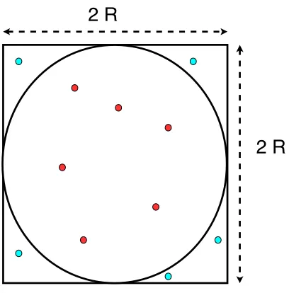
2R (see Fig. 3.1). A number of random points, {pi}, which lie within the square are drawn. A point,pi = (xi, yi), is counted inside the circle ifxi2+yi2≤R; otherwise outside. LetNin be the number of random points lie inside the circle and N be total number of the points. Then the
area of the circle is estimated very straightforward:
Ac=
Nin
N As (3.1)
Figure 3.1: A square of width 2R and a circle of radius R are shown. The points are randomly drawn. The red points are inside the circle, however, the others are outside of the circle. The ratio of the red points to the total number of points is equal to the ratio of the area of the circle to that of the square (in the limit that the number of points goes to the infinity).
several times and the average will be the estimated value of the area of the circle. Afterward,
one can estimate the numberπ. It is noteworthy that unlike deterministic methods, MC method
always gives results with a statistical error bars. However, as it can be seen from this simple example that MC integration approaches the problem in a so simple manner that one does not
have to deal with difficult analytic derivations. This simplicity and straightforwardness makes
MC the method of choice in many complicated problems.
3.1.1 Random Numbers
The MC method uses a random number sequence. A random number sequence can be defined
roughly as a sequence of numbers in which the number in the next iteration can not be preor-dained by the numbers at the current and past iterations. Despite this, the random numbers
generated by regular random number generator programming routines are not random in
real-ity since they are somehow already determined by the algorithms. Nevertheless, these random numbers generators are designed so that the number sequences carry some attributes of the
![Table 3.1:Some functions commonly used in the Jastrow correlation terms [6].](https://thumb-us.123doks.com/thumbv2/123dok_us/4164.1155036/68.612.205.427.95.182/table-functions-commonly-used-jastrow-correlation-terms.webp)