EIS consistency
Characterizing
environmental
impact
statements
for road projects in North Carolina, USA
Luis E Carrasco, Gary Blank and Erin O Sills
We evaluate consistency and patterns among a 20-year sample of EISs for road projects in North Carolina, USA. Applying multivariate sta-tistical methods, we find substantial variation in reporting of project and site characteristics, the EIS process itself, and types and definitions of impacts. We find a relationship between envi-ronmental impacts and bio-physical or geo-graphic factors. The relationship between predicted environmental impacts and economic factors suggests more environmental impacts oc-cur, or are identified, in high-income counties. Variables describing public involvement and completeness are associated mainly with the number of residential relocations required. Farmlands potentially impacted are reported in-consistently and are not reliable for comparison, so rural environmental impacts may be seriously underestimated.
Keywords: environmental impact assessment, environmental impact statements, environmental quality, highway projects, NEPA, multivariate analysis, North Carolina USA.
Luis E Carrasco (corresponding author) is a PhD student, Gary Blank and Erin O Sills are Associate Professors, North Carolina State University; E-mail: [email protected].
The authors wish to thank Ms Cynthia Roebuck and Mr Randy Turner at NCDOT for providing access to the EIS library and Dr Marcia Gumpertz from the Statistics Department at NC State for her help in the methodology.
HE US NATIONAL ENVIRONMENTAL Policy Act (NEPA) of 1969 was designed to increase federal environmental oversight of development activities in the United States, in res-ponse to concerns over their negative impacts and the lack of regulation. NEPA calls for an environ-mental impact statement (EIS) when the possibility of an environmental impact resulting from a major federal action has been identified. Use of federal funds in a state project, such as a highway, requires the proposing agency to adhere to NEPA standards even if the state has its own environmental policy act. Federal agency implementation of NEPA, how-ever, has varied considerably across agencies (Smythe and Isber, 2003).
Other documents, such as environmental assess-ments (EAs) or categorical exclusions (CEs), do not address the same scale of environmental impacts in proposed projects. CEs are for small projects, such as bridge replacements, and assume limited and be-nign environmental impacts. EAs are for projects, or more often subproject, judged to have unknown or minimal environmental impacts. Any subprojects with important impacts on the environment, includ-ing on endangered species or wetlands, would necessarily require an EIS.
In more than three decades since NEPA was es-tablished, the environmental impact process has been applied to numerous activities and, with few modifications and equivalent processes in some states, it is still effective in the USA. According to Cambridge Scientific Abstracts (2000), each year the federal government issues hundreds of environ-mental impact statements that are stored in the database Digests of Environmental Impact
State-ments. This database is updated bimonthly with
approximately 150 additional studies from different federal agencies.
Given the numbers produced, the quality of EISs has been discussed ever since documents started be-ing completed in the early 1980s but has been a more frequent focus of comment in recent years. For example, Tzoumis and Finegold (2000) find that federal agencies are not submitting EISs of consis-tent quality, according to the rating system used by the Environmental Protection Agency (EPA). Such inconsistency may well be a function of the incon-sistent implementation noted by Smythe and Isber (2003). For example, Atkinson et al (2000), studying treatment of biodiversity impacts in a sample of draft EISs, find inconsistencies and inadequacies in the documentation. These authors and others call for more systematic analyses of EISs to identify the pat-terns and explore possible reasons for these inconsis-tencies (Daini, 2000).
The study reported here arose from the question of whether statistical analyses of EIS documents could help identify underlying tendencies and pat-terns in the studies. This paper presents results of multivariate statistical analyses of EISs in the trans-portation sector in North Carolina. The transporta-tion sector impacts nearly all ecological zones and is a vital element of most human economic activities all over the world. Canter (1996) shows that 22.1% of all EISs filed in the United States between 1979 and 1991 were for the transportation sector, the highest percentage among all the federal sectors. Tzoumis and Finegold (2000) include EISs from the transportation sector in their study. They find that quality ratings given by the EPA decreased over the years for projects presented by the Federal Highway Administration, as well as by the USDA Forest Ser-vice and US Army Corps of Engineers.
Phillips and Randolph (2000) list three “key shortcomings” in NEPA implementation:
• project developers do not engage early with the NEPA process through interdisciplinary collaboration;
• studies lack rigorous science application and incorporation of ecological principles and tech-niques; and
• the administrative process does not encourage achievement of NEPA’s main goals.
They note that specialists criticize the NEPA process because it fails to integrate project design and envi-ronmental management practice. Bailey (1997), de-scribing the evolution of EIS in Australia and the USA, points out the importance of the relationship between the EIS process and its subsequent envi-ronmental management phase, suggesting that pro-ducing the EIS provides a set of management goals. Thus, the success of the subsequent project man-agement phase depends on the accomplishment of NEPA goals in the EIS phase. The Phillips and Randolph (2000) study suggests that environmental
and/or ecological management of projects could be improved by a meticulous analysis of NEPA imple-mentation by sector, as different types of project present their own particularities, with different points where improvements can be made. Hence the examination here of transportation documents.
Methodologies used in previous reviews of EISs
Three main methodological approaches have been used to evaluate the quality of, and patterns in, EISs, in addition to the method used by the EPA to grade EISs. Tzoumis and Finegold (2000) describe the en-vironmental review process created and employed by the EPA (as required by section 309 of the Clear Air Act) for grading EISs. This method consists of grading EISs according to two scales. The first, which evaluates the environmental impacts of the preferred alternative, is a four-point rating scale that includes: lack of objections (LO); environmental concerns (EC); environmental objections (EO); and environmentally unsatisfactory (EU). The second scale rates the adequacy of the information presented in the EIS. It consists of a three-point scale com-prised of: adequate; insufficient information; and in-adequate. According to these authors, this procedure is used by ten EPA regional offices throughout the United States.
Atkinson et al (2000) develop a simple semi-qualitative method to grade a sample of EISs from different federal agencies in the USA and evaluate their treatment of biodiversity. Their method con-sists of calculating the average of summed grades on 19 aspects of the treatment of biodiversity, as deter-mined by different evaluators. Using this method, a high score represents a document of high quality. This approach is appropriate when a high level of agreement exists among a multidisciplinary group. However, this subjective scoring system depends on the evaluators’ criteria and expectations.
Daini (2000) uses cluster analysis to find similari-ties in data structure from EISs for hydroelectric projects in the Trentino region of Italy. He finds that two out of three sections of EISs were treated con-sistently: project site information and environmental baseline information. The only section that showed significant differences was impact assessment, and these results suggest non-standard treatment of envi-ronmental impacts within the same region. Daini (2000) recommends close study of particular eco-nomic sectors to find any relationship between the elements of an EIS and its quality. He concludes that this type of study would be a great tool to formulate or improve guidelines for future development pro-jects. Our study builds on Daini’s (2000) approach by focusing on the transportation sector in the USA and applying two different methods of multivariate analysis.
and site characteristics, (b) the methods used for the EIS, and (c) the types and definitions of impacts. Second, using canonical correlation analysis, it ex-plores relationships among these three categories of ‘variables’ in the EIS process. Third, it uses princi-pal component analysis to identify other combina-tions of variables that explain variacombina-tions among EISs. As a result, it enables analysis of relationships among impacts identified in the EIS, the EIS pro-cess, and the economic and environmental character-istics of transportation projects.
Methodology
The methodology used in this study consists of the following six steps, explained in more detail below.
1. Collection and review of all EISs produced by the NCDOT from 1980 to 1999;
2. Identification of specific information (variables) provided in most of these EISs in three catego-ries: project and site information; information on the environmental assessment process; and pre-dicted environmental impacts;
3. Collection of data from the EISs, with each vari-able coded numerically;
4. Calculation of the percentage of EISs that
provided data on each variable and construction of a ‘completeness index’;
5. Evaluation of relationships between categories of variables with canonical correlation analysis; 6. Identification of factors underlying variation in
EISs with principal components analysis (PCA).
Collection and preparation of data
Between 1980 and 1999, the NCDOT submitted 43 EIS documents to the EPA. Those examined were all produced under guidance by the Federal Highway Administration as NEPA EIS projects. The EIS documents were obtained from the NCDOT library. To the extent possible, data were collected from fi-nal EIS documents. However, draft EISs were also used in this study when a final version was not available or did not exist. The EIS documents cov-ered a wide range of transportation projects, in rural and urban areas and in all three physiographic prov-inces of North Carolina (see Table 1).
Reviewing a sub-sample of ten EISs suggested that information in the 43 documents should be divided into the following categories for purposes of this study: site and project information; envi-ronmental assessment information and environ-mental impacts. Each of these categories includes information that is commonly assessed in studies of EISs. From all the variables available within each category, the set of variables in Table 2 was selected
Table 1. Location of road projects
Type of area Physiographic province
Coastal Plain
(CP)
Piedmont (PID)
Blue Ridge (BR)
Total type of area
Rural 7 (22%) 21 (66%) 4 (13%) 32 Urban 2 (18%) 9 (82%) 0 (0%) 11 Total
physiographic province
9 30 4 43 (100%)
Table 2. Consistency of reporting EIS components
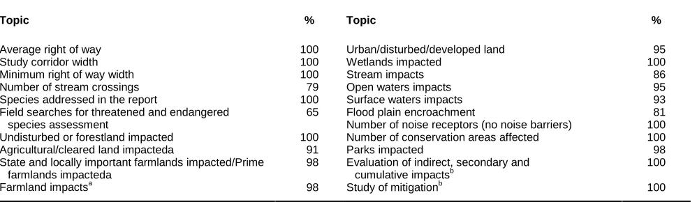
Topic % Topic %
Average right of way Study corridor width Minimum right of way width Number of stream crossings Species addressed in the report
Field searches for threatened and endangered species assessment
Undisturbed or forestland impacted Agricultural/cleared land impacteda
State and locally important farmlands impacted/Prime farmlands impacteda
Farmland impactsa
100 100 100 79 100 65 100 91 98 98
Urban/disturbed/developed land Wetlands impacted
Stream impacts Open waters impacts Surface waters impacts Flood plain encroachment
Number of noise receptors (no noise barriers) Number of conservation areas affected Parks impacted
Evaluation of indirect, secondary and cumulative impactsb
Study of mitigationb
95 100 86 95 93 81 100 100 98 100 100 Notes: a used as categories or subcategories
b addressed only conceptually
This study evaluates the consistency of
reporting on project and site
characteristics, methods used for the
EIS, and types and definitions of
impacts: it explores relationships
for data collection. These variables represent information likely to be important across a broad range of transportation EISs and were presented in a reasonably consistent manner, allowing data collection and coding.
Other important variables, such as impacts to farmlands, were also investigated. However, the EISs used very different methodologies for calculat-ing farmland impacts, includcalculat-ing categories that might overlap with each other or with different land uses. For instance, prime farmlands are classified by soil type, not by land use, so they may also include developed land. On the other hand, some counties may not have a soil or farmland classification, re-sulting in inaccurate or incomplete information. This point will be examined further later in the discussion.
For each variable, the percentage of documents that provided data is shown in Table 2. A new vari-able measuring the ‘completeness’ of the studies was created using the following procedure:
• In the original database, missing data in any study and in any field were coded as –1, and existing data were kept with their original numeric values.
• A second database was created from the original, transforming the values for each variable. All col-lected data were transformed to 1, and missing data values were transformed to 0.
• The newly transformed values for each study (or record) were totaled.
• The total value for each record was divided by the highest value found among all the records; thus, values for this new variable range from 0 to 1.
• The variable was labeled completion index (CI).
Because they were available consistently for all pro-jects, the following variables were selected for the analysis in each of the three categories:
• Site and project: physical province, cost of right of way, cost of construction, income per capita.
• Environmental assessment: specialists on team, endangered species addressed, field surveys con-ducted, public comments, completion index.
• Environmental impacts: forestlands impacted, wetlands impacted, residences relocated.
In particular, note that the environmental assessment variable labeled ‘public comments’ provides a measure of public participation and interest in the EIS process. Table 3 provides definitions for each of these variables.
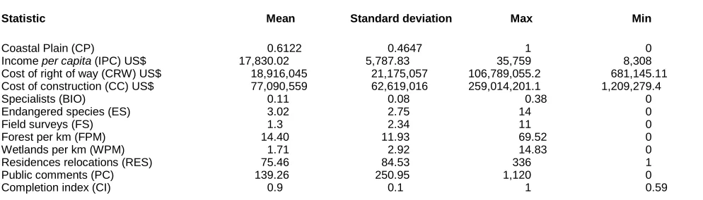
Many of the site and project variables are corre-lated with the scale of the project. To distinguish their effects from the effect of project size, the vari-ables were normalized as follows. Cost of right of way, cost of construction, acres of forest impacted, acres of wetland impacted, and residences relocated by project were divided by the road length (by km). The preferred reference variable would have been the size of the right of way, but this was not meas-ured consistently across studies, perhaps because of the different criteria used to estimate impacts to types of land. Table 4 provides acronyms and de-scriptive statistics for the normalized variables.
The variables for physiographic province were transformed into two dummy variables for Coastal Plain, and Blue Ridge and Piedmont. Blue Ridge was combined with Piedmont because only four pro-jects occurred in the Blue Ridge region.
Table 3. EIS components used as variables
Variable Description
Site and project
Right of way width of projected road measured in feet plus an additional margin of space in case changes in design are required Cost of right of way cost of acquisition of land within the right of way area of a preferred alternative, in 1982 dollars
Cost of construction cost of workforce, materials, and engineering for the construction of the preferred alternative, in 1982 dollars Physiographic province physiographic province of the project: Blue Ridge (BR), Piedmont (PID), and Coastal Plain (CP)
Income per capita average income per capita in the county of the project, from the Bureau of Economic Analysisa Environmental assessment
Specialist ratio ratio of environmental professionals to total professionals involved in the process of preparing the EIS Endangered species number of species in a designated federal conservation category, such as threatened or endangered, that are
mentioned in the EIS (not necessarily impacted by the project)
Field surveys number of field studies that sought evidence of endangered or threatened species in the area of influence of the proposed project or study corridor
Public participation number of comments received by the agency in charge of the EIS as counted by the agency Completeness index comparative ratio of the number of topics addressed in a given EIS relative to the most complete EIS Environmental impacts
Forestlands impacted estimated hectares of forestland that will be modified, partially or entirely, because of the construction of the road or preferred alternative
Wetlands impacted estimated hectares of wetland that will be modified, partially or entirely, because of the construction of the road or preferred alternative
Residences relocated number of residence properties that are located within the right of way and need to be relocated to allow the road construction
Most of the variables selected for the multivariate analyses showed non-normal distributions. Normali-zation of data was necessary to interpret the results of parametric tests with more confidence. Each vari-able’s distribution was determined using normal dis-tribution graphs and normal quantile plots. For the variables with exponential distributions, square root or logarithmic normalizations were chosen based on the final distribution of the data after transformation. The logarithmic transformation was used for all variables with similar logarithmic distributions.
Asdiscussedabove,onlyalimitedsetofvariables couldbeusedinthemultivariateanalyses.Other vari-ableswerenotreportedbyallstudiesorwerereported using inconsistentmetricsand definitions.This was particularly notablefor farmland categories and im-pacts.EventhefullsetofvariableslistedinTable2 does not captureall important aspects ofEISs from environmental, economic, or social perspectives.
Statistical analyses
The total sample size for the analyses described be-low was 43 EISs. Each of the statistical analyses was performed using the statistical software SAS. An al-pha level of 0.01 is interpreted as ‘very significant’ whereas 0.15 is interpreted as ‘significant’ for the PCA.
In canonical correlation analysis (CCA), the vari-ables were divided into groups, so the focus is on the association between any two groups of variables (Manly, 1986; Wichern, 1988). This contrasts with the cluster analysis used by Daini (2000), which seeks to divide the EISs (the individual observa-tions) into groups based on the values of the vari-ables for each study. Here the three categories of variable from EISs serve as the group for CCA.
The objective was to find whether any pair of groups has a statistically significant correlation. A significant canonical correlation between two groups may suggest a cause–effect relationship. For in-stance, a high canonical correlation between site and project, and environmental impacts would suggest that the occurrence of environmental impacts is causally linked to some of the variables in site and
project, which are relatively fixed in space and time. However, it is important to consider the nature of each variable to arrive at a reasonable interpretation.
An association and its strength are defined by the squared canonical correlation (R2) between the can-onical variables (or linear combinations) and its sta-tistical significance as defined by the p-value. Further interpretation of each canonical correlation was supported by calculating the partial correlations between each original variable and each canonical variable.
According to Manly (1986) and Wichern (1988), PCA is designed to reduce the number of variables that need to be considered to a small number of indi-ces (called principal components) that are linear combinations of the original variables. This method explains the variance-covariance structure of a set of multivariate data. Wichern (1988) points out that PCA often reveals relationships that were not previ-ously suspected and allows interpretations that would not ordinarily result. This method is thus a useful complement to the CCA.
In this study, PCA was used principally to iden-tify linear relationships of importance in the dataset. It was also used to infer the statistical importance of each variable, as identified by its eigenvector in each principal component. Partial correlations between variables were also examined to support interpreta-tion of each relainterpreta-tionship.
Table 4. Simple statistics of normalized variables
Statistic Mean Standard deviation Max Min
Coastal Plain (CP) 0.6122 0.4647 1 0
Income per capita (IPC) US$ 17,830.02 5,787.83 35,759 8,308 Cost of right of way (CRW) US$ 18,916,045 21,175,057 106,789,055.2 681,145.11 Cost of construction (CC) US$ 77,090,559 62,619,016 259,014,201.1 1,209,279.4
Specialists (BIO) 0.11 0.08 0.38 0
Endangered species (ES) 3.02 2.75 14 0
Field surveys (FS) 1.3 2.34 11 0
Forest per km (FPM) 14.40 11.93 69.52 0
Wetlands per km (WPM) 1.71 2.92 14.83 0
Residences relocations (RES) 75.46 84.53 336 1
Public comments (PC) 139.26 250.95 1,120 0
Completion index (CI) 0.9 0.1 1 0.59
Principal components analysis was
used to identify linear relationships of
importance in the dataset and to infer
the statistical importance of each
variable, as identified by its
eigenvector in each principal
component; partial correlations
Results
Theresultsbelowprovideausefulfirstassessmentof relationshipsandcharacteristicsofEISs,specifically inthetransportationsectorinNC.Canonical correla-tionanalysis wasconductedtoexplore relationships amongthethreecategoriesofvariables:siteand pro-ject, environmental assessment, and environmental impacts. Results of principal components analysis follow presentations of these relationships.
Site and project vs environmental impacts
CCA is used first to test for statistically significant correlations betweenlinearfunctionsofvariablesin twogroupsorcategories: siteandproject,and envi-ronmental impacts. Table 5 shows that the first
resulting canonical correlation between these two
sets of variables is moderate (0.53) anda very sig-nificant correlation according to its p-value (<0.0001).Thesecondcanonicalcorrelationshowsa small correlation (0.38) and is also very significant
(p-value=0.0007).Thefirstcanonicalcorrelation de-scribes 60.2% of the variability between these two sets of variables, and the second explains 32.3%.
These results suggest that the environmental impact variables (impacts to wetlands, forests and urban property) relate to the geographic location of the project (in the Piedmont or in the Coastal Plain). Furthermore, environmental impacts relate to eco-nomic characteristics of the project, represented here as cost of right of way and construction.
The analysis reported two linear functions or can-onical functions with coefficients for each variable within each category. These standardized canonical coefficients show the importance of each variable in their canonical linear function (Table 5). In this case, the first canonical correlation coefficients for site and project stress the importance of the variables Coastal Plain (CP) and cost of right of way (CRW).
On the other hand, the coefficients for the environ-mental impacts set stress the importance of impacts to wetlands (0.993) over the other two variables (forest impacted and residential relocations).
The second canonical function, although having a small correlation, shows the importance of the vari-ables Piedmont (as negative of CP), CCW, and resi-dential relocations as in the previous relationship. However, it gives more importance to impacts on forestlands than on wetlands, which makes sense from a regional point of view, because there are more forestlands than wetlands in the Piedmont of North Carolina.
Site and project vs environmental assessment
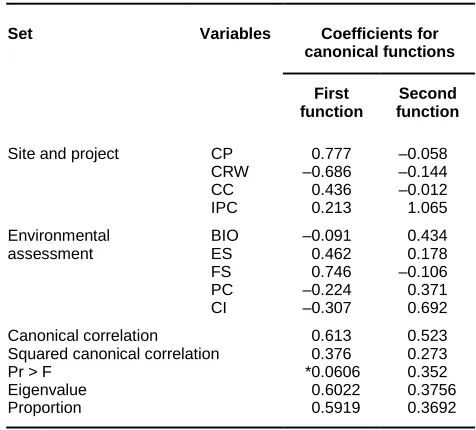
This subsection considers whether a canonical corre-lation exists between site and project and environ-mental assessment. The canonical correlation between these two sets of variables is moderate (R2=0.38) and significant at 15% (p-value=0.061). The second canonical correlation is small and not significant.
ThecoefficientsshowninTable6forthefirst can-onical correlation for site and project stress the importance of the variables CP (0.777) and cost of construction (CC) (0.436), as opposed to CRW (– 0.686). On the other hand, the coefficients of the first canonical function for the environmental as-sessment group give importance to the variables en-dangered species (ES) (0.462) and field surveys (FS) (0.746),asopposedtocompletionindex(CI)(–0.307) and public comments (PC) (-0.224) (Table 6).
Environmental impacts vs environmental assessment
The first canonical function shows a low correlation (0.339) between the variables in environmental assessment and environmental impacts (Table 7).
Table 5. Coefficients for canonical functions: site and project vs environmental impacts
Coefficients for each canonical functions Set Variables
First function
Second function
CP 1.023 –0.266 CRW 0.614 0.839 CC –0.023 0.124 Site and project
IPC –0.029 –0.090 FPM –0.070 0.424 WPM 0.993 –0.271 Environmental impacts
RES 0.310 0.817
Canonical correlation 0.73 0.62 Squared canonical correlation 0.53 0.38 Pr > F **<0.0001 **0.0007
Eigenvalue 1.150 0.617
Proportion 0.602 0.323
Table 6. Coefficients for canonical functions: site and project vs environmental assessment
Coefficients for canonical functions Set Variables
First function
Second function
CP 0.777 –0.058 CRW –0.686 –0.144 CC 0.436 –0.012 Site and project
IPC 0.213 1.065 BIO –0.091 0.434
ES 0.462 0.178
FS 0.746 –0.106 PC –0.224 0.371 Environmental
assessment
CI –0.307 0.692 Canonical correlation 0.613 0.523
Squared canonical correlation 0.376 0.273 Pr > F *0.0606 0.352
Eigenvalue 0.6022 0.3756
The size of the second correlation shown is very low and thus not worthy of interpretation. However, the p-values for both canonical correlations are signifi-cant at 15% (0.014 and 0.082).
Coefficients for the variables in environmental impacts stress the importance of impacts to natural resources, forest per km (FPM) (0.239) and wetlands per km (WPM) (0.358) as opposed to impacts on ur-ban resources represented by residential relocations (RES) (–0.885). Concerning the canonical variable environmental assessment and its individual vari-ables, the importance relies on the specialists (BIO) (0.371), and number of endangered species ad-dressed in the report (0.617), as opposed to the com-pletion index (–0.606).
Principal components analysis
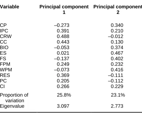
Principal components analysis is applied to all the variables listed in Table 8, transformed appropri-ately, plus the indicator variable for Coastal Plain
and the completion index. The first component explains 25.8% of the variation, and the first two components together explain nearly half (48.9%) of the variance. The rest of the components contribute relatively little explanatory power, which can be attributed to the large number of variables used in this analysis.
The coefficients for each variable in the first and second principal components are shown in Table 8. In the first component, the following variables are most important: income per capita (IPC) (0.391), cost of right of way per km (0.488), cost of construc-tion (0.443), and residential relocaconstruc-tions (0.369). This suggests a relationship among variables concerning the economic characteristics of the project and site (IPC, CRW, CC) and impacts primarily to property (RES) and secondly to forestlands (FPM) in the Piedmont. This relationship is supported by the bivariate correlation between CRW and RES of 58%, one of the highest in the data set.
The second principal component stresses the im-portance of geographic location (0.34 for Coastal Plain), linked to environmental assessment variables such as specialists in the team (0.373), endangered species assessment (0.467), and field surveys per-formed (0.402), as well as impacts to wetlands (0.416) and to forestlands (0.232). Another variable of importance in this analysis is the completion in-dex, which has a moderate weight in both the first component (0.266) and the second one (0.229). This weight suggests that completeness of a study is related to both environmental and economic charac-teristics of a project.
Discussion
Although produced by NCDOT, the 43 documents examined for this study all adhered to extant Federal Highway Administration (FHWA) guidelines for meeting NEPA requirements as interpreted by FHWA. Moreover, engineers and consultants en-gaged by NCDOT to assist in EIS preparation were trained in workshops specifically presenting FHWA procedures and expectations for EISs. Thus, the evaluation here focused on federal process for envi-ronmental impact assessment. Although North Caro-lina has enacted a State Environmental Policy Act (SEPA), the use of federal transportation funds for major highway projects necessitates following NEPA and coordinating with federal agencies in the planning and impact assessment process.
As noted above, EPA applies two scales to evalu-ate environmental impact stevalu-atements (Tzoumis and Finegold, 2000). The four point-scale actually rates the preferred alternative rather than the document it-self. The three-point scale broadly rates adequacy of information in EIS documents. Both broad scales provide little information about the quality of the process or specific data about the documents them-selves. Various studies of EISs have pointed to a
Table 7. Coefficients for canonical functions: environmental impacts vs environmental assessment
Coefficients for each canonical function
Environmental impacts Set Variables
First function Second function
FPM 0.239 0.613 WPM 0.358 0.521 Environmental
impacts
RES –0.885 0.422
BIO 0.371 –0.524
ES 0.617 0.664 FS 0.167 0.208 PC –0.169 –0.002 Environmental
assessment
CI –0.606 0.602
Canonical correlation 0.582 0.470 Squared canonical correlation 0.339 0.221 Pr > F *0.014 *0.082
Eigenvalue 0.512 0.284
Proportion 0.552 0.858
Table 8. Eigenvectors of principal components analysis
Variable Principal component 1
Principal component 2
CP –0.273 0.340
IPC 0.391 0.210
CRW 0.488 –0.012
CC 0.443 0.130
BIO –0.053 0.374
ES 0.021 0.467
FS –0.137 0.402
FPM 0.249 0.232
WPM –0.073 0.416
RES 0.369 –0.111
PC 0.205 –0.112
CI 0.266 0.229
Proportion of variation
25.8% 23.1%
need for more systematic research of the process and its products (Atkinson et al, 2000; Daini, 2000; Tzoumis and Finegold, 2000).
This study provides a quantitative examination of relationships among components of 43 environ-mental impact statements produced by NCDOT from 1980 to 1999 to find patterns that permit gaug-ing the quality of these studies. It applies statistical measures to address the commonality expected among such documents. However, such an approach necessarily cannot address the unique attributes of individual EIS studies. Thus, examining NCDOT EISs during this period offers a few challenges.
First, the practice of environmental impact as-sessment was rapidly evolving during the early 1980s, following adoption and implementation of NEPA regulations. NCDOT, like all state transporta-tion agencies, was following FHWA guidance, pre-sented through FHWA workshops and manuals that defined the agency’s idiosyncratic process. FHWA guidelines had to be adapted to the realities of state regulatory processes and data availability as they evolved in response to Environmental Protection Agency and other federal agency mandates and funding initiatives. Thus, practitioners producing NCDOT EISs were aiming at moving targets in terms of expectations for completeness.
As a second challenge, each project for which an EIS is prepared occurs in a unique landscape with project-specific characteristics, including dimen-sions of the project, advocates and opponents of the project, flora and fauna native to the project area, level of development in the project area, and purpose and need for the project. Such purposes and needs range from creating a bypass around an urban area to upgrading a stretch of rural highway on a new loca-tion for safety reasons. Such variability provides limited similarities on which to make effective com-parisons of the resulting EIS documents.
Third, the process of preparing EISs, while sub-ject to general timetable and milestone expectations, varies greatly from project to project, depending on circumstances that arise while the studies and com-pilation of the document are underway. Changes in regulations and in characteristics of a project study area can each affect the end product. Indeed, one of the main criticisms of the NEPA process is that it can result in delays that seriously impact proposed projects (Bregman, 1999).
In part, document quality may be a result of the systems in place. As part of the NEPA process, all the environmental impact statements require review and comments from several federal agencies to en-sure environmental protection and minimize, avoid, or plan to mitigate negative environmental impacts before initiating the projects. The goal of that review process is to integrate an environmental perspective in every proposed federal decision. However, be-cause most environmental impact studies have in-formation related to a specific time frame, a long administrative process can result in the EISs being
outdated and require that they be updated at addi-tional cost. In addition, reviewing agencies may re-quest expansions of the EISs, again resulting in additional costs for those amendments or extensions.
The quality of an EIS is a perceived value. In simple terms, an EIS is good when the information it provides is accurate, so that planners can make in-formed decisions regarding the use of natural, hu-man and/or economic resources. In this sense, lack of data or its inconsistency diminishes the quality of any document. Yet, in the EISs examined, only a fraction of all possible variables was complete or present in all the studies in such a way as to allow complete comparison among them. Here, the uniqueness of projects and the variability of their lo-cations are largely to blame and, in fact, some miss-ing data are probably more important than others.
Theperceptionofqualityisalsorelatedtotheease of reader access, the effectiveness of the language used, style employed, amount of graphic support, clarity of connections within the document, and other factors of rhetorical impact that add to, or de-tract from, perceived quality of an EIS. No acknowl-edged method exists for quantifying these matters and the effects they have on perception of quality in the documents examined. This study specifically avoids examining the rhetorical devices and stylistic dimensions of EIS documents produced by NCDOT.
It is important to bear in mind that the use of quantitative data can hardly reflect the complete characteristic range of a policy process such as NEPA. The analyst may need additional input, be it quantitative or qualitative, which may require sub-jective approaches or, better still, sound experience. Despite that, it is expected that quantifying charac-teristics not only of the EIS documents but of the process itself can provide valuable insights.
The approach here focuses on quantifiable aspects that require the fewest subjective assumptions. De-creasing the number of subjective assumptions in order to identify those elements of EISs can allow measurement of their quality. If nothing else, quanti-tative analysis poses a number of provocative ques-tions on which to build arguments for changes in process and products of environmental impact assessment.
Economic factors, impacts, and information quality
This analysis provides two different ways to charac-terize EISs. Both rely primarily on economic characteristics of projects. The first involves mainly impacts to property and the second impacts to natural resources.
Coastal Plain, to more expensive, higher-impact pro-jects more likely to be in the Piedmont. The positive coefficient for public comments in this first principal component suggests that public intervention in the EIS process is more prominent when impacts on properties are expected.
The second component shows a different relation-ship between economic and environmental factors. Income per capita and cost of construction are related in the same direction as impacts on natural resources (forests, wetlands, and endangered spe-cies). This relationship suggests that impacts on natural resources are more likely to be identified in areas with higher income per capita. The fact that wetlands and forests have to be filled or cleared might increase the cost of construction, but not nec-essarily the cost of the right of way, as these lands usually are less expensive than developed ground. However, potential impacts on endangered species could result from forest and wetland removal.
This relationship also shows that public comments (used here as an indicator of public involvement in the EIS process) occur more often when residence relocations are predicted than when impacts to envi-ronmental resources such as wetlands or endangered species are predicted, as supported by the first principal component. The second component also suggests that the relationship between impacts to natural resources and income per capita is strongest for projects in the Coastal Plain (as opposed to the Piedmont).
The completion index (CI), an indicator of the amount of information included in each EIS, appears in both components, although it seems to be more important in the first. This suggests that more infor-mation is collected when a project has more impacts on property than on natural resources. Note that the PCA excludes the year of the study, or a time trend, that could also help explain variation among studies.
Relationships with site and project
Canonical correlation analysis identified relation-shipsamonggroupsofvariablesthatareusually pre-sent in EISs. The squared canonical correlation betweencharacteristicsofthesiteandprojectandthe
environmentalimpactsfoundintheEISsuggeststhat environmental impacts (on wetlands, forests, and residences)arerelatedtowhethertheprojectisinthe Piedmont or inthe Coastal Plain.This geographical relationshipwasexpected,sincemorewetlandsoccur intheCoastalPlainthaninthePiedmont.
Likewise, environmental impacts are also related to economic characteristics of the project, repre-sented here as costs of both right of way and con-struction, and also income per capita. These correlations summarize the relationships suggested by the two principal components discussed above. The correlation between impacts and project costs cannot be attributed to size of the project, because both cost of right of way and cost of construction were normalized by size of the project.
Relatively low correlation between the character-istics of the site and project and the environmental assessment (0.38) suggests that the decision to in-volve more specialists in the EIS is not strongly related to location of the proposed project or income level in the project region. Furthermore, public in-volvement, as measured by public comments, does not seem to be a result of the regional or economic characteristic of a particular project but rather be-cause of impacts on private property.
On the other hand, the completion index might be related to specialists in the field and secondly to economic characteristics of the project site, such as cost of right of way, which would be supported by the PCA discussed above. This relationship suggests that a more complete EIS occurs when enough spe-cialists are involved in a project and in counties with relatively high income per capita because people, institutions, and agencies in these regions expect more thorough EISs.
Relationship between EA and environmental impacts
The CCA showed little statistical relationship
between the process of environmental assessment
and the environmental impacts identified. Thefacts that numbersofspecialists,endangeredspecies, and surveys had positive correlations withthe canonical coefficientfor environmentalimpacts, andthat pub-liccommentsandcompletionofinformationshowed negativecorrelationshavetobeinterpretedcarefully. In theory, we might expect a relationship between these categories in the same direction, as environ-mental impacts are supposed to be estimated from the results of environmental assessment or a part-icular methodology used to identify and quantify environmental impacts. In practice, however, it is desirable that methodologies should not affect the findings of environmental assessment. In this sense, the fact that environmental assessment and environ-mental impacts are not related is a positive finding. One possible interpretation for this result is that pub-lic comments, a variable exogenous to assessment of environmental impacts on natural resources, added noise to the data.
In the case of completion of information, this variable includes more factors than those that affect biodiversity directly. The EIS dataset comes from a wide geographic and economic spectrum; to analyze more direct cause–effect relationships between envi-ronmental assessment methodologies and predicted environmental impacts might require focusing on projects occurring within a smaller geographic area, hence exhibiting less variability.
Considerations for EIS practice
While discussion so far has focused on each particu-lar statistical analysis, this section addresses implica-tions of the overall results for EIS practice and identifies topics or issues that require more attention in the future to improve the EIS process itself. Such improvement is required if we expect more detailed or advanced treatment for biodiversity issues as some authors have suggested (Atkinson et al, 2000). Because those who produce EISs have continually acquired technical knowledge about the NEPA pro-cess through practical experience, however, it is pos-sible that some real improvements to EISs will only occur concerning those topics or issues that either legislation or the administrative process itself iden-tify as critical to improve.
Improvement might reacha limit oraneconomic constraintwithrespecttowhatislegallyrequiredfrom anEIS.Forexample,inanimpactassessment,onestep inscopingistoidentifythespeciesinaparticular pro-tectioncategoryintheareaoftheproject.Current prac-ticeinNorthCarolinarequireson-the-groundsearches forfederallylistedendangeredandthreatenedspecies if potential habitat exists in the study area.
However, searches of potential habitat are not re-quired for federal species of concern (FSC), nor for state-listed protected species if they are not federally listed as endangered or threatened. Although con-ducting searches for these species would certainly improve the coverage of biodiversity issues in EISs, the time and costs involved are viewed as prohibi-tively expensive. Only in rare circumstances, such as when scientific judgment suggests that a species will soon be federally listed, will such searches be con-ducted. Yet even the number of searches that must be conducted may be suspect.
Federal and state agencies maintain lists of threat-ened and endangered species in geographic areas based on the information they store in their data-bases, regardless of whether information is current. Such lists are taken as the official reference for scheduling and performing field surveys for EIS. Logically, use of old information can result in the EIS being less accurate and lead to poor project de-cisions. These lists are costly to update, however, as they depend on expensive periodic field surveys. Thus, to achieve reliable EISs, funds need to be directed to source database maintenance, but such allocation has not been the responsibility of agencies typically proposing projects.
Another area of possible improvement involves consistent reporting of all natural resources. As methods of environmental assessment have crucial importance in EISs, they determine quality of tech-nical information required to forecast environmental impacts. Different classifications used to refer to the same resources (for instance, farmlands, water bod-ies, or forestlands) made detailed comparisons among documents used in this study difficult, as the data were too variable, having different nomencla-tures or being measured in different ways.
In effect, lack of concern about impacts to certain types of landscape may be revealed by how land-scape components are treated in EISs. Officially, in the documents studied, this lack of concern seemed to translate into tolerance for inconsistent terminol-ogy and unclear reporting of potential impacts to a less valued resource. Subcategories of farmlands overlapped each other frequently. Unlike impacts to forest and wetland, conversion of farmland to high-way and other uses appeared to generate relatively little concern.
Here the fault may lie with agency definitions and conflicting, or at least different, schemes for as-sessing the value of these resources. Such agency definitions and practical applications are difficult to alter once they are embedded in administrative procedures. NCDOT and the practitioners preparing EIS documents are not at fault. While it is likely that open farmlands are more highly valued in high-income counties when residential development raises the value of open space and the characteriza-tion as open space gains greater attencharacteriza-tion, this termi-nology was seldom used.
Clearly, the true success of an EIS is measured by its ability to forecast actual environmental impacts that occur and can be measured in the field. These forecasts are unlikely to be precise, especially if de-tails of road construction are not designed until after the EIS is approved.
However, it seems appropriate to ask what kind of technical information is needed in an EIS to forecast environmental impacts accurately and make appro-priate design decisions. Perhaps EISs need to overestimate environmental impacts so the responsible agency commits to keep those impacts within reasonable and predicted limits. In any case, an EIS should serve as a guide to ensure that necessary development will happen with the least amount of environmental damage. This issue seems somewhat critical, given that indirect and cumulative impacts of highway projects were covered only generally in EISs until recent years.
in the final design of a project would make the EIS process more useful.
Finally, to produce a document of quality, authors of EISs need to collect accurate environmental data, which is expensive and time consuming. Recent de-velopment of applied environmental sciences has provided varying methods to make data collection a little more affordable. Using biologic indicators and increasing use of geographic information systems (GIS) (for instance, for forest and wetland delinea-tion and to estimate areas that will be impacted by a road project) may add accuracy and therefore quality to the process, while at the same time lowering costs. Yet GIS and other data-inquiry systems, which depend on keeping databases accurate and updated, are only as reliable as the inventoried information.
Future methodologies should include feedback from the parties involved in the EIS production and review process including state agencies, environ-mental subcontractors and county representatives. Further, the quality of information in EISs may need to be analyzed or measured with other methodolo-gies that focus on the process and quality control procedures in place.
Recommendations
The following recommendations are extracted from the previous discussion. Three of them aim to im-prove understanding of the assessment process:
• Focus on smaller and more homogeneous geo-graphical areas to analyze more specific issues within the EIS process.
• IncludeinthedocumentstheupdatedEPAreview criteriatogradeEISsthusmakingtheEISprocess betterunderstoodbythedifferentpartiesinvolved.
• Acknowledge and make public those issues that are crucial in the EIS process, regardless of the proposing agencies, thereby centering the atten-tion of the public or agencies on the main envi-ronmental impacts assessed and perhaps shortening review processes.
Five of the recommendations could improve the process itself:
• Provide consistent information in future EISs, try-ing to standardize the variables or topics to cover in each project.
• Homogenize treatment of different topics in EIS by interdisciplinary collaboration. For instance, treatment of indirect or cumulative impacts could be improved by introducing best methodologies applied among agencies. This way, different fed-eral agencies would learn from their own experi-ence and documents could be better standardized.
• Ensure that environmental impacts are addressed with the same effort, regardless of level of income in the project area, cost of project or type of im-pacts (to natural resources or to human property).
• Consistently include federal species of concern to improve the treatment of impacts to protected species.
• Ensure that all the federal agencies have accurate and current information regarding the status of natural resources, by enhancing state govern-ments’ ability to provide current data.
Conclusions
From 1980 to1999, 43environmental impact state-mentswerecompletedforNorthCarolinabythestate DepartmentofTransportation. Thirtyoftheprojects were inthe Piedmont andninein theCoastal Plain, whileonlyfouroccurredintheBlueRidgeprovince. Three quarters of the projects were in rural areas.
Multivariate analysis of these EISs suggests that predictedenvironmentalimpacts,suchasimpactson forests and wetlands, are related to the particular physiographic region where a project is planned.
Impacts arealsorelatedtoeconomicfactorssuch as incomeper capitaandthecosts ofright ofwayand
ofconstruction.While therelationshipbetween geo-graphical regionandenvironmentalimpacts was ex-pected, that betweenenvironmental impacts andthe economiccharacteristicsofaprojectwasnot.This re-lationship suggeststhatmoreenvironmentalimpacts occurredorwereidentifiedinhigh-incomecounties.
Furthermore, as measured by the number of pub-lic comments, more pubpub-lic involvement tends to oc-cur in the EIS process when impacts on residential properties are identified. EISs for projects in high-income counties also appear to be more thorough, as measured by the completeness index. On the other hand, information pertaining to farmland potentially impacted is reported inconsistently in NCDOT documents and cannot be used reliably for com-parison purposes. Thus, environmental impacts in rural and probably lower-income counties may be underestimated.
The characteristics of the environmental assess-ment process do not have any strong relationship with the projected impacts on wetlands, forestlands,
Future methodologies should include
feedback from the parties involved in
the EIS production and review
and residential relocations. Apparently, regardless of the number of specialists involved, the number of species reviewed, or the number of field surveys, the EIS process identifies similar impacts, with quanti-ties of impacts determined by type of project and site. Environmental assessment quality does show a moderate statistically significant correlation with site and project information. These findings reflect posi-tively on the environmental assessment process in North Carolina, as the potential impacts identified by that process are sensitive to site and project char-acteristics but independent of the details of the envi-ronmental assessment process.
References
Atkinson, S, S Bathia, A Schoolmaster and W Waller 2000. Treatment of biodiversity impacts in a sample of environmental of US environmental impact statements. Impact Assessment and Project Appraisal, 18(4), 271–282.
Bailey, J 1997. Environmental impact assessment and man-agement: an underexplored relationship. Environmental Management, 21(3), 317–327.
Bregman, J 1999. Environmental Impact Statements. Florida: Lewis Publishers.
Canter, L 1996. Environmental Impact Assessment. New York: McGraw-Hill.
Cambridge Scientific Abstracts 2000. EIS: Digests of environ-mental impact statements. Available at <http://www.csa.com/ detailsV3/eis.html>, last accessed 30 August 2000.
Daini, P 2000. Environmental impact assessment for hydroelectric power plants in Trentino (Italy) 1990-1997: similarity and clus-tering of studies, sites and projects. Impact Assessment and Project Appraisal, 18(1), 43–60.
Manly, B F J 1986. Multivariate Statistical Methods: a primer. London: Chapman and Hall.
Phillips, C and J Randolph 2000. The relationship of ecosystem management to NEPA and its goals. Environmental Manage-ment, 26(1), 1–12.
Smythe, R and C Isber 2003. NEPA in the agencies: a critique of current practices. Environmental Practice, 5(4), December, 290–297.
Tzoumis, K and L Finegold 2000. Looking at the quality of draft environmental impact statements over time in the United States: have ratings improved?. Environmental Impact As-sessment Review, 20(5), 557–578.