A Study on Applicability of Soil FEM Model to Evaluate Uplift Behaviour of
NPP Buildings against Large Earthquake
Takaki Tojo1, Koji Inoda2, Naohiro Nakamura1 Kohei Matsumoto2, and Takuya Suzuki1
1
R&D Institute, Takenaka Corporation, Japan ([email protected]) 2
The Kansai Electric Power Co., Inc., Japan
ABSTRACT
In the current seismic design of Japanese nuclear power plants, various methods are used for estimating the seismic response of buildings in accordance with the level of basemat uplift. The level of basemat uplift is an important design criterion and can be determined using the ground contact ratio. When the contact ratio is small, a three-dimensional finite element method (hereafter 3D FEM) soil model is used. However, this model cannot be used for contact ratios of under 35%, and there are no alternatives applicable to such low contact ratios in the current design methods. The limit of the 3D FEM soil model is determined by comparison with a different theoretical analysis method, the green function method (hereafter GFM). In previous studies, the GFM could not be assessed with the multi-node building model in cases where the ground contact ratio was less than 35%. The GFM lost its stability because it was easily influenced by vibration characteristics of the building. In this study, we conducted seismic response analysis using the GFM and 3D FEM with a one-node building model for low ground contact ratios.
INTRODUCTION
In the seismic design of nuclear power plant buildings in Japan, the behavior of the plants in response to severe earthquakes must be accurately predicted. The level of basemat uplift, which can be determined using the ground contact ratio (!), is an important design criterion. This is the ratio of the contact area of the basemat bottom to its entire area when the level of uplift is largest (Japan Electric Association (2008)).
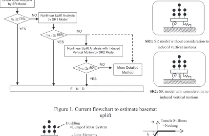
Fig. 1 shows the flowchart used in the current design method for estimating the seismic response of buildings in accordance with the level of basemat uplift. With decreasing !, induced vertical motion occurs due to basemat uplift, along with variation in the horizontal response of the building. These analysis models consider soil-structure interaction, and are required to accurately estimate both phenomena, the basemat uplift and the induced vertical motion. In the case of ! = 65%, the estimation of uplift can be made using a nonlinear Sway-Rocking (hereafter SR) model without considering the induced vertical motion (SR1 in the figure), which is thought to be negligible. In the case of 65% > !" 50%, the estimation can be made using an SR model by considering the induced vertical motion (SR2 in the figure) (Tanaka et al. (1995) and Momma et al. (1995)). When the ! value is below 50%, more detailed investigations are required due to the difficulty in estimating the induced vertical motion. The 3D FEM soil model, using joint elements between the basemat and the soil (shown in Fig. 2), can be used as a method for low values of ! (Japan Electric Association (2008)). However, it cannot be used under ! = 35%. There are no methods applicable to such low contact ratios in the current design methods.
#! < 35% is required. This report examines the applicability of the analytical method using the 3D FEM soil model to cases where ! is less than 35%.
Figure 1. Current flowchart to estimate basemat uplift
(a) Concept of FEM Model (b) Concept of Joint Elements
Figure 2. Concept of the 3D FEM Soil Model (More Detailed Method)
INVESTIGATION POLICY
In terms of ! values of 35% or more, the applicability of the 3D FEM soil model is assessed by comparing results with the green function method (GFM) (Shimomura and Tajimi, 1988), a theoretical solution method based on the elastic wave theory, and considered the limit of congruence between response analysis results of building models in a multi degree of freedom (hereafter MDOF) system. Here, analysis was possible using the 3D FEM soil model for low !#values (30% or lower), but the GFM lost its stability near the 30% level. Due to the absence of a comparison model, the GFM ! of 35% was set as the limit (Nakamura et al. (2007)).
The GFM is likely to be affected by the vibrational characteristics of the structure; thus, in the models using the MDOF system with low !#values, the solution tends to become unstable. When viewed as a model in a single degree of freedom (hereafter SDOF) system to simplify the vibrational characteristics of the structure, cases with smaller ! values could be analyzed. Therefore, this report examines the applicability of the 3D FEM soil model for low ground contact ratio caseswith the targeted building being a simplified model that consists of the linear structure on a semi-infinite soil in an SDOF
SR2: SR model with consideration to induced vertical motions SR1: SR model without consideration to
induced vertical motions
E N D Nonlinear Uplift Analysis
by SR1 Model
Nonlinear Uplift Analysis with Induced Vertical Motion by SR2 Model
!NL2 50%
YES NO
More Detailed Method
!NL! 65%"
!L 75%" Linear Uplift Analysis
by SR Model
NO
NO YES
YES
"
k
#!
Tensile Stiffness =Nothing!
Compressive Stiffness =Extremely High! Building
=Lumped Mass System
Joint Elements
system. Seismic response analysis is conducted with the GFM and the 3D FEM soil model to compare the response characteristics.
ANALYTICAL CONDITIONS
Modeling Of Building And Soil
The targeted analysis model of this study is a nuclear power plant building on a hard rock site. The building is modeled by beam element in an SDOF system, and for both the GFM and the 3D FEM soil model, the building’s basemat is a rigid body. The soil is a uniform half space whose shear velocity (Vs) equals 2000 m/s.
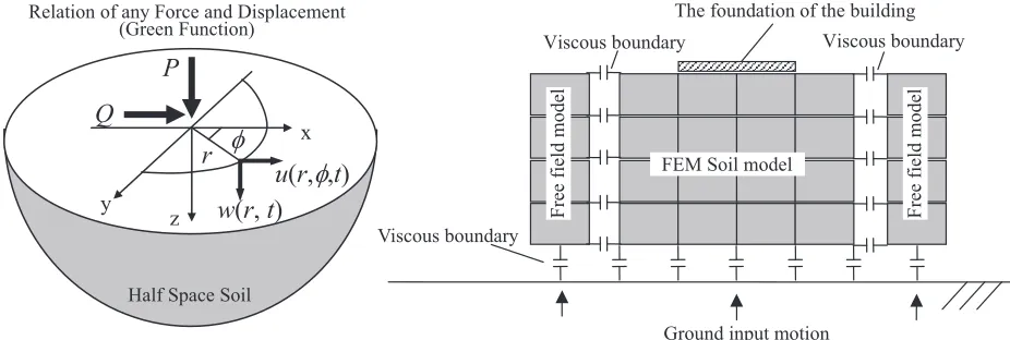
In the GFM, the soil is assumed as a 3D semi-infinite elastic half space that does not resist tensile stress. Fig. 3 shows the concept of the GFM. In the 3D FEM soil model, the first-order, 8-node isoparametric elements (hexahedral elements) are used as the solid elements. With regard to the basemat uplift, the nonlinear characteristics (shown in Fig. 2) are indicated by joint elements arranged between the basemat and the soil. Fig. 4 illustrates the boundary conditions of the FEM soil model. The viscous boundaries of the lateral sides of the FEM soil model are connected to free field models with the same physical properties. The bottom of the soil model is also a viscous boundary (Lysmer et al. (1969)).
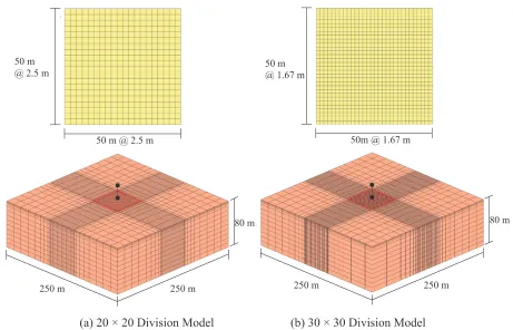
For both the GFM and the 3D FEM soil model, two cases are used as the analysis model: one with a basemat mesh of 20 equal divisions, and one with 30 equal divisions. Fig. 5 shows the 3D FEM soil model with the mesh division diagram of the basemat. Tables 1 and 2 show the physical properties assigned to the building and the soil. The building damping for both models is equal to Rayleigh damping and is set to h = 5%.
Input Seismic Motion
In this investigation, several input seismic motions which are made by multiplying some amplification factors to the original input motion are used. The original input motion is defined at the soil surface level, and the maximum horizontal acceleration of that is 550 gal. These seismic waves assume a horizontal input from a single direction. In the 3D FEM soil model, a correctional wave is created to generate the seismic motion necessary at the surface level, and this is input to the bottom end of the FEM soil model. Fig. 6 shows the acceleration time history and acceleration response spectrum of the original input seismic motion.
Figure 3. Concept of Green Function Method! ! ! Figure 4. Boundary Condition of FEM Soil Model
r
$%
P
Q
y z
x
u
(
r
,
$
,
t
)
w
(
r
,
t
)
Half Space Soil
Relation of any Force and Displacement (Green Function)
Ground input motion Viscous boundary
Viscous boundary Viscous boundary
The foundation of the building
FEM Soil model
F
re
e
fi
el
d
m
o
d
el
F
re
e
fi
el
d
m
o
d
(a) 20 × 20 Division Model (b) 30 × 30 Division Model
Figure 5. 3D FEM Soil Model (Upper: Mesh Pattern of Foundation Area, Bottom: Total Model)
Table 1. Building Properties! ! ! ! ! ! ! ! ! Table 2. Soil Properties
*1) Values for Bottom Fix Condition.
(a) Acceleration Time History (b) Response Spectrum (h = 5%)
Figure 6. Input Seismic Motion
Foundation Width [m]
50 × 50
Building Weight [t]
50,000
Foundation Weight [t]
150,000
1st Natural
Frequency
*1Hor. [Hz]
5.0
Vert. [Hz]
12.0
Building Height [m]
40.0
Vs[m/s]
2000
!
0.35
"
[t/m
3]
2.7
250 m 250 m80 m 50m @ 1.67 m
50 m @ 1.67 m 50 m
@ 2.5 m
50 m @ 2.5 m
250 m 250 m
80 m
-600 -300 0 300 600
0 10 20 30 40 50 60 70 80
Time (s)
Investigaion seismic motion (Max. 550 gal, 27.67 s)
A
cc
. (
g
al
)
0 500 1000 1500 2000
0.01 0.1 1 10
Investigaion Seismic Motion
A
cc
el
er
at
io
n
(
g
al
)
VALIDATION OF ANALYSIS MODEL
First, the validity of both the FEM soil model and the joint elements expressing the nonlinearity of the basemat uplift behavior is confirmed.
Confirmation Of FEM Soil Model
The horizontal and rotational impedances computed using the FEM soil model are compared with the theoretical results obtained by vibrational admittance theory (Tajimi (1959)). The impedance in each direction is obtained under the uncoupled condition. The impedance of the FEM soil model is calculated as follows:
1. The response displacement of the massless rigid basemat on the soil surface against the forced motion is calculated in the time domain.
2. The spectrum of the displacement is calculated by the Fourier transform and is then divided by the spectrum of the forced motion.
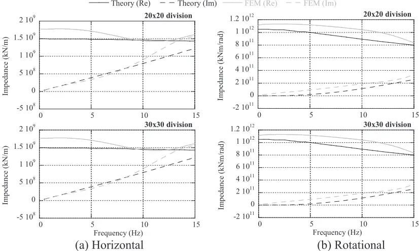
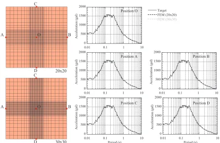
Fig. 7 shows the comparison of the horizontal and rotational impedance of the basemat on the Vs = 2000 m/s soil surface for the 20 × 20 and 30 × 30 division models. The impedance of the FEM soil model (“FEM” in Fig. 7) generally agreed quite well with the theoretical values (“Theory” in Fig. 7).
Next, a seismic response analysis is conducted using the input motion, corrected as discussed in the previous section (shown in Fig. 6). The response waves at representative points on the ground surface of the model are compared with the targeted input wave. Fig. 8 shows the comparison of the response spectra of the response waves on the soil surface between the FEM soil model (“FEM” in Fig. 8) and the targeted wave (“Target” in Fig. 8). Consequently, it was confirmed that the response waves corresponded quite well to the targeted wave at all points and that the response waves were almost uniform at these points on the soil surface.
(a) Horizontal (b) Rotational
Figure 7. Comparison of Soil Impedance (Upper: 20 × 20 model, Bottom: 30 × 30 model)
Theory (Re) Theory (Im) FEM (Re) FEM (Im)
-2 1011 0 2 1011 4 1011 6 1011 8 1011 1 1012 1.2 1012
0 5 10 15
20x20 division
Im
p
ed
an
ce
(
k
N
m
/r
ad
)
-2 1011 0 2 1011 4 1011 6 1011 8 1011 1 1012 1.2 1012
0 5 10 15
30x30 division
Im
p
ed
an
ce
(
k
N
m
/r
ad
)
Frequency (Hz) -5 108
0 5 108 1 109 1.5 109 2 109
0 5 10 15
20x20 division
Im
p
ed
an
ce
(
k
N
/m
)
-5 108 0 5 108 1 109 1.5 109 2 109
0 5 10 15
30x30 division
Im
p
ed
an
ce
(
k
N
/m
)
Figure 8. Comparison of Acceleration Response Spectra of Soil Surface (h= 5%)
Confirmation Of Joint Elements
The nonlinear characteristics of the basemat uplift are estimated by the joint elements installed between the FEM soil model and the lower end of the basemat of the building. In this section, the validity of the joint elements is investigated.
It would be ideal if the joint elements were completely rigid for compression and their stiffness value was 0 for tension. However, in an actual analysis, a finite and adequate value needs to be established for the compressive stiffness. In this study, a value of around 50 times the static value of the vertical soil impedance is defined as the adequate compressive stiffness (Nakamura et al. (2007)).
The joint elements are installed between the massless rigid basemat and the FEM soil model. After basemat sinkage due to the self-load of the building model, the nonlinear characteristics of the basemat uplift caused by static moment loading were computed. The validity of the computed values is estimated by comparing them with the results obtained from the GFM and approximate solution that is verified by previous research (Japan Electric Association (2008)).
Fig. 9 and Fig. 10 show M–$ (moment and rotational angle), !-–M (ground contact ratio and moment), and !–$ (ground contact ratio and rotational angle) relations computed from the static loading. The result of the GFM is almost the same for the 20 × 20 and 30 × 30 division models. Moreover, the result of the GFM corresponds quite well to that of the approximate solution for low (30% or lower) ground contact ratios (“Green” and “Approx”, respectively, in Fig. 9). The result of the FEM soil model corresponds well to that of the GFM in all cases (“FEM” and “Green”, respectively, in Fig. 10).
From the above, the validity of the nonlinear behavior of the FEM soil model uplift was confirmed. 0
500 1000 1500 2000
0.01 0.1 1 10
Target FEM (20x20)
FEM (30x30)
A
cc
el
er
at
io
n
(
g
al
)
0 500 1000 1500 2000
0.01 0.1 1 10
A
cc
el
er
at
io
n
(
g
al
)
0 500 1000 1500 2000
0.01 0.1 1 10
A
cc
el
er
at
io
n
(
g
al
)
Period (s)
0 500 1000 1500 2000
0.01 0.1 1 10
A
cc
el
er
at
io
n
(
g
al
)
0 500 1000 1500 2000
0.01 0.1 1 10
A
cc
el
er
at
io
n
(
g
al
)
Period (s)
O O A
A
B
B C
D
D C
20x20
30x30
Position O
Position A Position B
(a) M–
$relation (b)
!–Mrelation (c)
!% $relation
Figure 9. Comparison of Static Investigation (GFM)
(a) M–
$relation (b)
!–Mrelation (c)
!% $relation
Figure 10. Comparison of Static Investigation (FEM Soil Model)
NUMERICAL RESULTS OF SEISMIC RESPONSE ANALYSES
In this section, the applicability of the 3D FEM soil model to evaluate uplift behavior in cases where !is 35% or lower is investigated by carrying out seismic response analyses. When input seismic motion gradually increases, the characteristics of uplift behavior and building response for both the GFM and the 3D FEM soil model are compared
Comparison Of Uplift Behavior
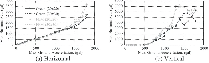
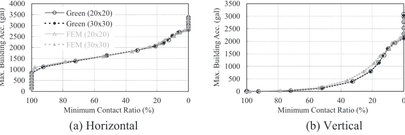
Fig. 11 describes the relationship between the input level and the minimum !. It can be seen that ! results from the 3D FEM soil model and the GFM are highly compatible, even at low ! (below 30%) and regardless of basemat divisions. The relationship between maximum input acceleration of the ground surface and the maximum response acceleration of the nodal point of the building top and the basemat is shown in Fig. 12 and Fig. 13 for the horizontal and vertical directions, respectively. Figs. 14 and 15 describe the relationship between the minimum ground contact ratio and the maximum response acceleration of those nodal points for the horizontal and vertical directions, respectively.
As can be seen for both models in Fig. 12, the maximum acceleration of the structure increases in response to the input seismic motion in the horizontal direction; on the other hand, in the vertical direction, it increases drastically when input level rises to 600 gal or greater. This is a response to the uplift behavior
0 1 107 2 107 3 107 4 107 5 107
0 5 10-5 1 10-4 1.5 10-4 2 10-4
R o ta ti o n al M o m en t (k N m )
Rotational angle (rad)
0 20 40 60 80 100
0 5 10-5 1 10-4 1.5 10-4 2 10-4
G ro u n d C o n ta ct R at io ( % )
Rotational angle (rad) 0 20 40 60 80 100
0 1 107 2 107 3 107 4 107 5 107
G ro u n d C o n ta ct R at io ( % )
Rotational Moment (kNm)
Joint ElementsStatic Moment LoadingMassless Rigid
Approx Green (20x20) Green (30x30) 0 20 40 60 80 100
0 5 10-5 1 10-4 1.5 10-4 2 10-4
G ro u n d C o n ta ct R at io ( % )
Rotational angle (rad) 0 20 40 60 80 100
0 1 107 2 107 3 107 4 107 5 107
G ro u n d C o n ta ct R at io ( % )
Rotational Moment (kNm) 0
1 107 2 107 3 107 4 107 5 107
0 5 10-5 1 10-4 1.5 10-4 2 10-4
R o ta ti o n al M o m en t (k N m )
Rotational angle (rad)
and is called induced vertical motion. Where the input level rises above 1700 gal, induced vertical motion shows some discrepancies, but it can be seen that the two models correspond well at ranges below the minimum ! values of 35% (set as the current applicability limit for the 3D FEM soil model) (see Fig. 14). The number of divisions of the basemat has little influence in both analytical methods.
In contrast to the building response (shown in Fig. 12), horizontal response shows discrepancies from input acceleration from approximately 1300 gal and for vertical response from approximately 700 gal (Fig. 13). The discrepancy in vertical acceleration is especially large. This is because the basemat receives the shock of contact after uplift without any internal damping. Consequently, there are variances in the responses of the GFM and the 3D FEM soil model. However, as the response of the 3D FEM soil model is somewhat larger than that of the GFM, the 3D FEM soil model conservatively evaluates the uplift behavior.
Figure 11. Relation of Maximum Ground Acceleration to Minimum Contact Ratio
(a) Horizontal (b) Vertical
Figure 12. Relation of Maximum Ground Acceleration to Maximum Building Acceleration
(a) Horizontal (b) Vertical
Figure 13. Relation of Maximum Ground Acceleration to Maximum Basemat Acceleration
0 500 1000 1500 2000 2500 3000 3500
0 500 1000 1500 2000
Ma
x.
Bui
ldi
ng
Acc
.
(g
al
)
Max. Ground Accelertation. (gal) 0
500 1000 1500 2000 2500 3000 3500
0 500 1000 1500 2000
M
ax
.
B
u
il
d
in
g
A
cc
.
(g
al
)
Max. Ground Accelertation. (gal)
0 1000 2000 3000 4000 5000 6000 7000 8000
0 500 1000 1500 2000
M
ax
.
B
as
em
at
A
cc
.
(g
al
)
Max. Ground Accelertation. (gal) 0
500 1000 1500 2000 2500 3000 3500 4000
0 500 1000 1500 2000
M
ax
.
B
as
em
at
A
cc
.
(g
al
)
Max. Ground Accelertation. (gal) 0
20 40 60 80 100
0 500 1000 1500 2000
M
in
. C
o
n
ta
ct
R
at
io
(
%
)
Max. Ground Accelertation. (gal)
Multiplied Seismic Motion Joint Elements
Green (20x20) Green (30x30) FEM (20x20) FEM (30x30)
(a) Horizontal (b) Vertical
Figure 14. Relation of Minimum Contact Ratio to Maximum Building Acceleration
(a) Horizontal (b) Vertical
Figure 15. Relation of Minimum Contact Ratio to Maximum Basemat Acceleration
Comparison Of Building Response
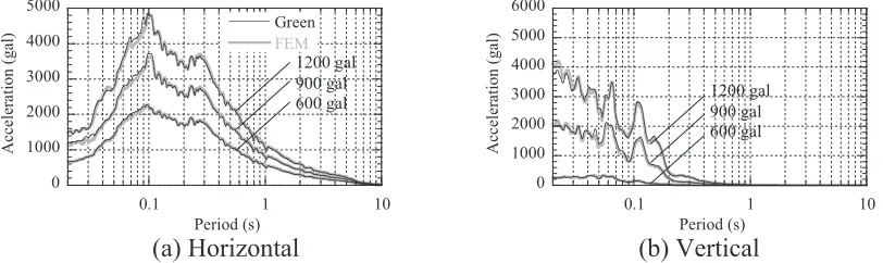
Fig. 16 shows the acceleration response spectrum (h = 5%) of the nodal point of the building top for input levels: 600, 900, and 1200 gal, where the minimum ! becomes approximately 55%, 15%, and 5%, respectively, for both horizontal and vertical responses in the 20 × 20 division model. From Fig. 16, it can be seen that the horizontal and vertical responses in the GFM and 3D FEM soil model correspond well, even where ! falls below 30%.
Fig. 17 shows the acceleration response spectrum (h = 5 %) of the nodal point of the basemat for vertical and horizontal responses in a 20 × 20 division model. From Fig. 17, although the responses of 3D FEM soil model correspond relatively well to that of the GFM for both directions in the same way as Fig. 16, the response of vertical direction is about the same level as that of horizontal one for both the GFM and 3D FEM soil models. This is because impulsive responses occur by basemat uplift and coming down. However, in this study, the nonlinear characteristics represented as local nonlinearity of the soil are not considered; thus; the responses are possibly evaluated somewhat conservatively than in reality.
On the other hand, the response in high-frequency components disappears in the response of the building top. This is considered to have disappeared due to internal damping of the building. There are sort of discrepancies of the basemat uplift behaviour between the GFM and 3D FEM soil model for the lower ! values, but discrepancies are relatively small. The 3D FEM soil model is able to appropriately evaluate the uplift behavior for low ! values (30% or lower).
0 500 1000 1500 2000 2500 3000 3500 4000
0 20 40 60 80 100
M
ax
.
B
as
em
at
A
cc
.
(g
al
)
Minimum Contact Ratio (%)
0 1000 2000 3000 4000 5000 6000 7000 8000
0 20 40 60 80 100
M
ax
.
B
as
em
at
A
cc
.
(g
al
)
Minimum Contact Ratio (%) 0
500 1000 1500 2000 2500 3000 3500
0 20 40 60 80 100
M
ax
.
B
u
il
d
in
g
A
cc
.
(g
al
)
Minimum Contact Ratio (%) 0
500 1000 1500 2000 2500 3000 3500 4000
0 20 40 60 80 100
M
ax
.
B
u
il
d
in
g
A
cc
.
(g
al
)
Minimum Contact Ratio (%) Green (20x20)
Green (30x30) FEM (20x20) FEM (30x30)
(a) Horizontal (b) Vertical
Figure 16. Building Acceleration Response Spectrum (h = 5%, 20 × 20 Model)
(a) Horizontal (b) Vertical
Figure 17. Basemat Acceleration Response Spectrum (h = 5%, 20 × 20 Model)
CONCLUSIONS
This report is a comparison of the uplift characteristics between the 3D FEM soil model and the GFM.From the above investigation, we obtained following findings:
1. With the building model in an SDOF system, the GFM can be applied to ! values of less than 30%.
2. The response of the 3D FEM soil model corresponds to that of the GFM when the contact ratio is nearly 0%.
3. The 3D FEM soil model is applicable to the evaluation of uplift behavior in cases where ! is nearly 0%.
REFERENCES
Lysmer, J., Kuhlemeyer, R., (1969), “Finite Dynamic Model for Infinite Media,” Journal of Engineering
Mechanics Div., ASCE, 95, pp.959-977
Momma, T., Shirahama, K., et al., (1995), Transactions of SMiRT13, Session K, pp.49-54
Shimomura, Y., Tajimi, H., (1988), Proceedings of 9th World Conference of Earthquake Engineering, Tokyo-Kyoto, Vol.III, pp.471-476
Tajimi, H., (1959), “Basic Theories on Aseismic Design of Structures,” Report of Institute of Industrial
Science, Tokyo Univ., Vol.8(4), pp.170-215, (in Japanese)
Tanaka, H., Maeda, I., et al., (1995), Transactions of SMiRT13, Session K, pp.43-48
Nakamura, N., Ino, S., et al., (2007), “An Estimation Method for Basemat Uplift Behaviour of Nuclear Power Plant Buildings,” Journal of Nuclear Engineering & Design, Vol.237, pp.1275-1287
Japan Electric Association., (2008), Technical Code for Seismic Design of Nuclear Power Plants
JEAC4601-2008, pp.105-106, (in Japanese)
0 2000 4000 6000 8000 10000
0.1 1 10
A
cc
el
er
at
io
n
(
ga
l)
Period (s) 0
2000 4000 6000 8000 10000 12000 14000 16000
0.1 1 10
A
cc
el
er
at
io
n
(
g
al
)
Period (s) 600 gal 900 gal 1200 gal
600 gal 900 gal 1200 gal FEM
Green
0 1000 2000 3000 4000 5000 6000
0.1 1 10
A
cc
el
er
at
io
n
(
g
al
)
Period (s) 0
1000 2000 3000 4000 5000
0.1 1 10
A
cc
el
er
at
io
n
(
g
al
)
Period (s)
600 gal 900 gal 1200 gal
600 gal 900 gal 1200 gal FEM