Bayesian entropy for spatial sampling design of environmental data
Montserrat Fuentes, Arin Chaudhuri and David M. Holland
1Institute of Statistics Mimeo Series No. 2571
SUMMARY
We develop spatial statistical methodology to design large-scale air pollution monitoring networks with good
predictive capabilities while minimizing the cost of monitoring. The underlying complexity of atmospheric
processes and the urgent need to give credible assessments of environmental risk create problems requiring
new statistical methodologies to meet these challenges. In this work, we present a new method of ranking
various subnetworks taking both the environmental cost and the statistical information into account. A
Bayesian algorithm is used to obtain an optimal subnetwork using an entropy framework. The final network
and accuracy of the spatial predictions is heavily dependent on the underlying model of spatial correlation.
Usually the simplifying assumption of stationarity, in the sense that the spatial dependency structure does not
change location, is made for spatial prediction. However, it is not uncommon to find spatial data that shows
strong signs of nonstationary behavior. We build upon an existing approach that creates a nonstationary
covariance by a mixture of a family of stationary processes, and a propose a Bayesian method of estimating
the associated parameters using the technique of Reversible Jump Markov Chain Monte Carlo. We apply
these methods for spatial prediction and network design to ambient ozone data from a national monitoring
network in the eastern US.
1Montserrat Fuentes is an Associate Professor at the Statistics Department, North Carolina State University (NCSU), Raleigh, NC 27695-8203. Tel.:(919) 515-1921, Fax: (919) 515-1169, E-mail: [email protected]. Arin Chaudhuri is a researcher at SAS, Cary, NC. David M. Holland is a senior statistician at the U.S. Environmental Protection Agency, RTP, NC. This research was sponsored by a National Science Foundation grant DMS 0353029 and by a US EPA award R-8287801.
1
Introduction
Environmental monitoring agencies around the world maintain large-scale air monitoring networks to assess
the efficacy of regulatory controls, determine current levels and trends, and provide air quality inputs to
risk assessment and source attribution analyses. However, these networks need to be managed such that
changing priorities and needs, both national and local, can be accommodated with the understanding that
there could be constraints in future funding for these networks. The proposed reduced network should
maintain sufficient spatial information to ensure reasonable statistical inference about air pollution. A
major criterion for modifying an existing network is the quality of the spatial predictions, and minimizing
the monitoring costs of obtaining such predictions or ensuring that monitoring continues in areas with high
pollution levels. In this work, we propose a new method for ranking various subnetworks (most informative
subsets) using an entropy measure of the spatial information and giving priority to monitoring sites with
high pollution values. Given this optimization criterion, a heuristic algorithm for determining near optimal
subnetworks of different sample sizes is described.
The spatial configuration of final subnetworks is heavily dependent on the underlying model for spatial
covariance. Complex, atmospherically driven pollutants are not expected to have simple, stationary forms of
spatial covariance. We build upon an existing approach for modeling underlying nonstationary covariance,
or heterogeneous covariance structure over large spatial ranges, by using a mixture of stationary processes.
Properties of this approach are given, along with a method for estimating the covariance parameters using
a Reversible Jump Markov Chain Monte Carlo (RJMCMC) approach. These methods are applied to ozone
design values for 1997-1999 observed at 513 monitoring sites in the eastern U.S..
The basic problem of air quality monitoring design is selecting the number and spatial configuration
of sites to allow, in some quantitative sense, optimal predictions of the air quality field subject to certain
constraints on monitoring resources. The design literature contains several different approaches for design.
The idea of using entropy in the context of experimental design goes back to at least Lindley (1947) and
Bernardo(1979). Caselton and Zidek (1984), Guttorp et al. (1993) and Zidek et al. (2000) developed the
maximum entropy design approach by modeling observations at different monitoring locations as a
have considered different approaches for network design. Warrick and Myers (1987) and M¨uller and
Zimmer-man (1999) considered design criteria for precise estimation of attributes of the semivariogram that affect
kriging. Others have considered design approaches under the assumption that the semivariogram is known
(Bras and Rodriguez-Iturbe, 1976; Yfantis, Flatman, and Behar (1987); and Cressie, Gotway, and Grondona,
1990). The design criteria considered by these authors are generally either the average kriging variance or
the maximum kriging variance over a region of interest. Wikle and Royle (1999) considered time-varying
or dynamic designs to evaluate the efficiency of allowing monitoring locations to change with time. Nychka
and Saltzman (1998) considered geometric space-filling designs and M¨uller (1999) investigated approximate
or simulation based approaches for optimal design using utility functions. The approach presented here
uses ideas from information and entropy theory integrated into a Bayesian framework for spatial prediction
incorporating the uncertainty of the covariance parameters. Given the regulatory need to maintain sites
near air quality standards, we give priority to retaining these sites. Our primary objective to downsize the
existing network, although these techniques could be applied to augment the network and select the most
informative sites for additional monitoring sites.
This paper is organized as follows. In Section 2 we introduce the scientific problem that motivated this
research and describe the data. In Section 3 we propose a fully Bayesian framework for selecting optimal
reduced networks. In Section 4 we extend this framework for network design to account for constraints,
including environmental cost. In Section 5 we discuss the design optimization problem. In Section 6 we
introduce our model for spatial nonstationarity. Section 7 presents an application using an air pollution
dataset.
1.1
Entropy as a measure of information
IfY is an uncertain, random quantity or vector of such quantities, andf(y) is the probability density function
ofY,then uncertainty aboutY can be expressed by the entropy ofY’s distribution,
H(Y) =
−f(y)log(f(y))dy.
For a distribution with low spread and a sharp peak near the mode, the mode provides a good indication
region where a ”typical observation” might lie could be quite large. In general, among a given family of
distributions the members with higher spreads have higher entropy. A nice exposition of the statistical
significance of entropy is given by Theil and Fiebig (1984). Thus, among all distributions having support in
the interval [a,b] we expect the uniform distribution on [a,b] to have the maximum entropy. We illustrate
this fact with few examples:
• IfY ∼N(µ, σ2),then,
H(Y) = 0.5(log(2π)−1) +log(σ).
Hence, the entropy is an increasing function of the variance
• IfY ∼U[a, b],then,
H(Y) = log(b−a).
The entropy function is an increasing function of the width of the interval.
2
Data
As national monitoring priorities and funding changes, it has become critical to optimize resources
avail-able for national monitoring networks. Thus, there is an urgent challenge to provide credible statistical
approaches for reducing or downsizing existing monitoring networks to find the most informative reduced set
of monitoring sites that will still meet multiple objectives of major monitoring programs. Here, we consider
downsizing the National Air Monitoring Stations/State and Local Air Monitoring Stations (NAMS/SLAMS)
(U.S. Environmental Protection Agency, 2003) ozone (O3) network. NAMS/SLAMS is the major source of
O3 data in the U.S. and monitorsO3at approximately 800 sites in the conterminous U.S. to determine
com-pliance with theO3, assess regional transport, and for use in estimating trends in this pollutant. Although
most NAMS/SLAMS sites are located in urban and suburban areas where air quality is influenced primarily
by local sources, some sites are located in rural areas to characterize regional air quality.
Tropospheric ozone continues to be one of the most significant air pollutant concerns in the United States.
Figure 1: Locations of 513 ambient ozone monitoring sites.
levels ofO3not only affect people with impaired respiratory systems, but healthy adults and children as well.
The U.S. Environmental Protection Agency (EPA) first set ozone National Ambient Air Quality Standards in
1971. These include primary standards to protect human health, and second standards to prevent ecological
and agricultural damages. In July 1997, EPA strengthened the O3 national ambient air quality standard
(NAAQS) based on scientific evidence showing adverse health effects from exposures allowed by the existing
standard. The new standard was defined in terms of 8-hour averaging times: the 3-year average of the
annual fourth-highest daily maximum 8-hour average ozone concentration is less than .08 parts per million
(ppm). This 3-year average is usually referred to as the ozone ”design value”. The maximum daily 8-hour
average ozone concentration is the highest of the 17 possible running 8-hour daily average concentrations.
We investigate new reduced designs usingO3 design values from 1997 to 1999 for 513 NAMS/SLAMS sites
3
Fully Bayesian approach for network design
We present a fully Bayesian approach for monitoring network design, taking into account the potential lack
of stationarity of the environmental process of interest (ozone, in this case), and some monitoring constraints
by using a utility function.
Consider a Gaussian spatial process{Z(x) :x∈D⊂ R2},with meanE[Z(x)] =µ(x).In the application
presented in this paper, the mean is a polynomial function on x. The covariance of Z( ) depends on a
parameterθ, cov[Z(x)Z(y)|θ] =Cθ(x, y). We put a prior distribution onθ,θ∼π( ). We observe the process
at locationsx1, x2, . . . xN, that is we have a vector of observationsZ= (Z(x1), Z(x2), Z(x3), . . . , Z(xN)). In
the problem of environmental network design we have to choose a subset of{x1, x2, . . . xN}of a given size such
that the loss of statistical “information”, here defined as entropy-utility, is minimal. For many atmospheric
processes, the spatial covariance function is nonstationary, in the sense that the spatial structure changes
with location. In Section 6, we present a nonstationary covariance model that is used in the proposed entropy
design framework.
3.1
The posterior predictive distribution
Consider the following Bayesian framework
Y ∼f(y|θ), θ∼π( ).
That is, we have a random variableY,whose density is given by a parametric formf(y|θ),andπ( ) is a prior
distribution forθ. In the Bayesian setup, the marginal density ofY at the pointy∗,is given by,
f(y∗|θ)π(θ)dθ.
However, after having an observation of the variable of interest,Y =ywe updateπ(θ) toπ(θ|y),and obtain
the posterior predictive density. So, if we observe a realization ofY,say y,the posterior predictive density
ofY at a pointy∗, after having observedy,is defined as,
fP(y∗) =
f(y∗|θ)π(θ|y)dθ.
Sampling from the posterior predictive density is easy, if we can sample from the posterior distribution
from the posterior distributionπ(θ|y),sayθ∗, and then we generate an observationy∗,fromf(y∗|θ∗). Thus,
y∗ is a sample from the posterior predictive density.
3.2
Fully Bayesian Network design
Our goal is to select an optimal subnetwork i of size k < N under a Bayesian framework by considering
all subsets of size k of (x1, . . . xk). We calculate the entropy of the posterior predictive density of Si =
(Z(xi1), Z(xi2). . . Z(xik)) and choose the subnetwork with the maximum posterior predictive entropy. Sites
with high uncertainties, which are generally more difficult to predict, are retained. Sites with smaller
uncertainties are eliminated from the subnetwork. This has the desirable predictive feature of excluding
sites characterized by high entropy values or higher uncertainties.
Let g() be the predictive posterior density of Si. In calculating the entropy ofg(), we should point out
that ifS1, S2, . . . , Sp is a sample fromg(). Then,
1 p
p
i=1
−log(g(Si))
is an unbiased estimator of the entropy ofg().Therefore, if we can compute the value of g( ),and generate
a sample from g( ), we should be able to estimate the value of the entropy of g(). Even though, we cannot
explicitly compute the value of g() at any point, say s0,we can still estimate its value using the following
approach:
• First, we generate a sampleθ1, . . . θk,from the posterior distribution ofθ.
• Then, the posterior predictive density can then be estimated as
ˆ
g(s0) = 1 k
k
i=1
f(s0|θi).
We estimate the posterior predictive entropy as
1 p
p
i=1
−log(ˆg(Si)).
However, since log(ˆg(Si))= log(g(Si)), the above expression may not be unbiased. Then, since
1 k
k
i=1
converges almost surely to the value of the posterior predictive density ats0, ask→ ∞for each s0, we can
then get good estimates by choosingklarge enough.
4
Utility of a Design
For a potential designS,we define a utility functionU(S). We selected a utility function that gives higher
priority or weight to sites with measurements near the NAAQS for ozone. Other utility functions such as
minus the monitoring cost could be used. Following Zidek et al. (2000), it seems natural to determine an
optimal design by maximizing a combined monitoring objective:
H(S) +γU(S),
where γ is a utility to entropy conversion factor. However, there is no natural way to choose γ, and we
decided to pursue modifications to this approach that are detailed in the following Section.
4.1
The utility function
Our objective is to choose a final design that gives more weight to sites that are more likely to exceed the
NAAQS for ozone. Thus, given a locationx0 we define the utility as
u(x0)=a0exp((z(x0)−c1)/h) ifz(x0)≤k0
=a1exp((z(x0)−c0)/h) ifz(x0)> k0
Wherec0,c1,a0,a1, k0are constants depending on air quality standards andhis a bandwidth parameter.
This utility function assigns more weight to sites with observations that are more likely to be out of compliance
with AQ standards. We define the utility of a subnetwork as the sum of the utilities of the sites in the
subnetwork,
U(S) =
x∈S
4.2
Preference relationships between designs
We would like to meet the dual objectives of maximizing the posterior predictive entropy while giving priority
to sites with highO3observations. Theentropy-utility combination for a designS, (H(S), U(S)) is a point
in R2 . However, it is not clear how to simultaneously achieve both purposes. Therefore, we introduce
a preference relationship on R2 to choose between any two designs, S1 and S2. Our goal is to select a
subnetwork of sites characterized by both high entropy and high utility. If S1 and S2 are two designs, an
obvious property any such preference relationship (say>>) must satisfy is:
• H(S1)> H(S2) andU(S1)> U(S2) thenS1>> S2.
If the entropy of one design is higher, but the utility value is lower,
H(Si1)> H(Si2) andU(Si1)< U(Si1).
then we base our decision on the relative gain in entropy versus the relative loss in utility value. If
(H(Si1)−H(Si2)) (H(Si1) +H(Si2)) >
(U(Si2)−U(Si1)) (U(Si1) +U(Si2)).
Then,
Si1>> Si2.
If the reverse inequality holds, then we have
Si1<< Si2.
When the ratios are equal, then we are indifferent to the choice between the two designs and we consider
the two designs equivalent to each other,
S1∼S2,
and we pick one design at random.
5
Optimization problem
To this point, we have discussed a network design criterion that can be used to define a useful subnetwork
Typ-ically, these design optimization problems for large sample sizes are highly formidable and pose enormous
computational problems. Many previous design efforts have applied simple one-at-a-time addition and
dele-tion procedures, that often lead incorrect soludele-tions. We could consider a sequence of reduced networks,
eliminating one station at a time, with subsequent calculation of the entropy associated with each of the
resulting networks. Then choose the natural cut-off for the number of sites by inspecting a plot of entropy
vs. number of sites. Another method of searching the design space is to sample blocks of design
param-eters. We will denote with d= (d1, . . . , dn) a vector of indicators specifying which stations remain in the
network (di= 1) and which do not (di= 0). WithN stations we have 2N possible designs. For instance for
N = 80 we could partition the design vectordin, eight blocksd= (d1, . . . , d8). We choose a new value of
dj given currently imputed values fordi, i=j, the covariance parameters (θ) and future data. Eachdj has
210 = 1024 possible values, we would need to evaluate the 1024 possible designs using the information-base
criteria, or any other approach. This is essentially Gibbs sampling (see Gelfandet al, 1990), since we are
conditionally updating the design. Ko et al. (1995) discussed an exact algorithm for determining maximum
entropy designs based on establishing the upper bound and incorporating this bound in a branch and bound
method. This approach can find the exact solution that maximizes entropy for relatively small sample sizes,
but it could not be implemented in our current setting, since we have a relatively large network. Thus, here
we use a simulated annealing (SA) approach. SA is a heuristic maximization method. It has been inspired
by the technique of slowly cooling a liquid to the lowest possible energy state. The different values a function
can take are considered possible energy values, and the optimal value is reached by using a random search
in an intelligent way. Suppose f() is a function we want to maximize. Let S = (s1, . . . , sk) be the set of
points where it attains a maximum. The goal of SA is to construct a non-homogeneous Markov chain that
converges towardsπ∞(), a uniform distribution overS.
5.1
The simulated annealing algorithm
Consider a sequence {Tn}, called a cooling schedule, converging slowly to 0. We start with an initial
subnetworkSi1. Then at theith step,
• IfSi1<< Si2,then we update the value ofSi1 toSi2.
• IfSi1>> Si2,then we updateSi1 toSi2 with probability
exp ⎛ ⎝−
H(Si1)−H(Si2)
H(Si1)+H(Si2)−
U(Si2)−U(Si1)
U(Si1)+U(Si2)
Tn
⎞ ⎠.
Initially, when Tn is large, the probability of jumping to an inferior point is higher, but since Tn →0 the
probability of jumping to an inferior point should become small after enough iterations. Various choices
for the cooling schedule have been suggested in the literature, we use here a geometric cooling schedule,
Tn =T0cn, for c = 0.8. To find the initial subnetwork for our SA algorithm, we use the geometric
space-filling design approach as described by Nychka and Saltzman (1998).
6
Modeling nonstationarity
In this section, we present a covariance model to characterize the potential lack of stationarity of the
environ-mental spatial process in the entropy network design framework. We assume the space domain of interestD
is divided into small subgrids,R1, . . . , Rn centered at the nodesr1, . . . , rn.The following equation describes
the model we use, which is an extension of the model proposed by Fuentes (2001) (see also Fuentes, 2002),
Z(x) =Z0(x) +√α
n
i=1
K(x−ri)Zi(x), (1)
Z() is the process of interest, and Z0( ), Z1( ). . . Zn( ) are underlying unobservable stationary processes,
which are mutually independent and Gaussian, and explain the spatial structure of Z in each one of the
subregionsRi. K(x−ri) is a weight function, e.g., the square inverse distance betweenxandri. HereZ0( )
is a background stationary process, and
√
α
n
i=1
K(x−ri)Zi(x)
is the nonstationary component of our model. We further assume that the stationary processesZ0( ), Z1( ), . . . , Zn( )
have a Matern covariance (Mat´ern, 1960),Ci(x−y), with parameterθi for eachZi
Ci(x) =τi2I0(x) + σi
2ηi−1Γ(ηi)(2η 1/2
i |x|/ρi)ηiKηi(2η 1/2
whereIis an indicator function, that takes the value 1 whenx= 0 and it is zero otherwise,Kηi is a modified
Bessel function (Abramowitz and Stegun, 1964, pp. 374-379), |x| =x21+x22 denotes de modulus of the
vectorx= (x1, x2). The parameterτi2is called the nugget parameter, and explains the microscale variability
and measurement error. The parameterρimeasures how the correlation decays with distance; generally this
parameter is called the range. The parameter σi is the variance of the random field, i.e. σi =var(Zi(x)),
and is usually referred to as thesill. The parameterηimeasures the degree of smoothness of the processZi,
which becomes smoother with higher values ofηi. Whenηi equals 12, the Mat´ern model corresponds to the
exponential covariance function. The Gaussian model is the limiting case of the Mat´ern asηi→ ∞
Ci(x) =σse−|x|2/ρ2i.
Parameters of the process
We assume, that givenn, thenstationary processesZ1( ), Z2( ), . . . , Zn( ) are Mat´ern with range
param-eters ρ1, . . . ρn, partial sill parameters σ12, . . . σn2, nugget parameters τ12, . . . τn2 and smoothness parameters
η1, . . . ηn respectively. The locations r1, . . . rn are npoints in our domain, that we call the centers of the
process. The critical parameterαmeasures the deviation from stationarity – for a nearly stationary
distribu-tion we expectαto be small. This parameter was not included in the previous version of this nonstationary
model as introduced by Fuentes (2001).
We observe the nonstationary process Z( ) at m locations x1, . . . xm. That is we have observations
Z(x1), Z(x2). . . Z(xm) wherex1, x2. . . xmarempoints in the plane. From eq. (1) we derive the form of the
covariance betweenZ(xj) andZ(xk) wherexj andxk are any two the points where we observe our process.
Note that
E(Z(xj)Z(xk)) =E({Z0(xj) +√α
n
i=1
K(xj−ri)Zi(xj)}
× {Z0(xk) +√α
n
i=1
K(xk−ri)Zi(xk)}).
Let us denote the stationary covariance of the processZi( ) byCi( ). By our assumption of mutual
indepen-dence of theZi( )’s the covariance betweenZ(xj) andZ(xk) simplifies to
C0(xj−xk) +α
n
i=1
Hence, the vector (Z(x1), . . . Z(xm)) is a multivariate normal distribution with covariance Σm×m = (σjk).
From above it follows that
σjk=C0(xj−xk) +α
n
i=1
K(xj−ri)K(xk−ri)Ci(xj−xk).
6.1
Choice of the Kernel function
For our kernel functionK,we choose the Epanechnikov kernel given by2
K(u) = 2 π
1 h2(1− |
u h|
2)+
Here,his a bandwidth parameter. The choice of the bandwidth is important; large values of the bandwidth
lead to oversmoothing, and small values to undersmoothing. We use the criterion developed by Fuentes and
Smith (2001) to choose the bandwidth. They propose using l
√
2
when the process is observed on an uniform
grid of width l. However, since our data are not on a grid, we calculate for each point the distance to the
nearest neighbor, that is, if we observe our process at locationsx1, . . . xm, we calculatel1, . . . lm, wherel1 is
the distance of the point closest tox1amongx2, . . . xmand so on. We choose l
√
2
as our bandwidth, where
l is the median of l1, . . . lm. This criterion for choosing the bandwidth coincides with the one proposed by
Fuentes and Smith (2001) when the data lie on a grid.
6.2
Covariance Parameter Estimation
6.2.1 Bayesian Framework
We construct a Bayesian framework from our model formulation to estimate the covariance parameters. The
parameters of our model are described by the following vector
θ= (n, α, r1, . . . , rn, ρ0, . . . ρn, σ20. . . σn2, τ02. . . τn2, η0, . . . ηn)
We assume there is a compact rectangle D ⊂ R2 which defines our domain of interest and we are not
interested in the values of our process outsideD. In our applications D is obtained as the bounding rectangle
of the points where we observe the process. Note that the dimension of the above vector is 4n+ 5,and it
depends on the first coordinaten,which is the number ofcentersof the process. Thus, our parameter vector
is of a variable dimension. We choose a Poisson prior forθ.
Prior Distributions:
1. the prior forn,the number of centers, is a Poisson(λ),whereλis given a conjugate Gamma hyperprior
with meanaand shape parameterb.
2. Given n,thencenters,r1. . . rn are i.i.d uniformly distributed over the domainD.
3. Givenn,the partial sill parameters,σ02, . . . , σn2 are given i.i.d diffuse inverse gamma priors with mean
ms and shape parameter 2.
4. Givenn,the nugget parameters,τ02, . . . , τn2 are given i.i.d diffuse inverse gamma priors with meanmn
and shape parameter 2.
5. Givenn,the range parameters,ρ0, . . . ρn are given i.i.d inverse gamma prior with meanmrand shape
parameter 2.
6. Given n,the smoothness parameters,η0, . . . ηn are given i.i.d uniform on the set{0.5,1.0,1.5,2.0,2.5}
7. αis given a prior distribution that is uniformly distributed on the interval [0,1]
Note that, n ∼ Poisson(λ) and r1, . . . , rn being distributed uniformly over D, given the value of n, it is
equivalent to assume thatr1, . . . , rn are distributed as a Poisson process overD with a constant rate λ. If
we have more information about the number and the spatial distribution of theri’s one might put a Poisson
process prior on (r1, . . . rn),with non-constant rate functionλ(x, y), where the rate functionλ(x, y) reflects
the knowledge about the distribution of thecenters. The Mat´ern covariance is very sensitive to changes in
the smoothness parameter, a continuous prior for this parameter offers computational challenges. Thus, we
work with a discrete prior based on analyses of similar datasets. For the partial sill and range parameters,
we use diffuse Inverse Gamma priors (with shape parameter 2). Note that Inverse Gamma distributions
with shape parameter 2 have infinite variance. Our inference aboutθ is based on its posterior distribution,
is made by constructing a Markov Chain which has the posterior distribution as its stationary distribution.
However, since our parameter has a variable dimension, the usual Markov Chain Monte Carlo methods do
not work. Thus, we use a RJMCMC approach developed by Green (1995) that constructs a Markov chain
with a distribution of a specified variable dimension distribution as the stationary distribution. The stages
of our approach to estimate the covariance mixture are:
(stage 1)updating the local covariances of the mixture components (θi), for a fixedn,
(stage 2)adding or dropping a mixture component,
and we iterate through stage 1 and 2. We judge convergence using the Brooks and Guidici (2000) approach.
7
Application
We apply the entropy-utility design approach to 1997-1999O3design values to find optimal subnetworks of
the original network of 513 monitoring sites. This approach involves:
1. modeling the design values as a nonstationary spatial process Z,allowing the covariance parameters
to change with location to explain the lack of stationarity. The process Z would have a covariance
functionC given in (3), that is a mixture ofnstationary covariance functions;
2. projecting the site coordinates using the Lambert projection;
3. modeling the mean function ofZ(x) as a polynomial onxof degree 3;
4. applying the RJMCMC approach to estimaten,the number of nodes that determine the center of the
subregions of stationarity.
In this case the estimated value of n is 3. Figure 2 shows the location of the 3 nodes: in the
north-east (node 1); in the southern part of the domain (node 2); and in the Midwest (node 3). This indicates
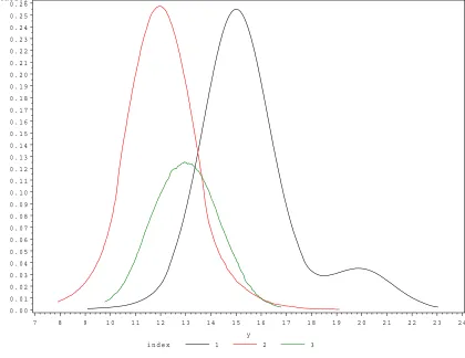
that there are three zones of nonstationarity. The posterior mean of the parameter α was .9. Figures 3
to 5 show the posterior distributions for the partial sill, range and nugget parameters for all nodes, using
subregions of stationarity, so we fixed this parameter at .5 to simplify the entropy computation. The partial
sill corresponding to subregion 3 has more uncertainty associated to it (see Figure 3), probably due to the
proximity of the edge of our domain. Subregion 1 (North-east) shows larger values for the partial sill. The
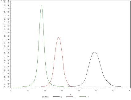
range of autocorrelation for the subregion of stationarity corresponding to node 1 is significantly smaller than
for node 3 (Figure 4), probably due to the spatial heterogeneity in the North-East because of the proximity
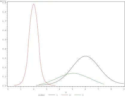
to the coast, and the presence of big cities. The nugget for subregion 2 is significantly smaller (Figure
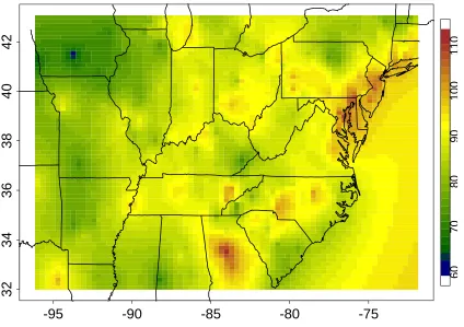
5). Figure 6 shows the map of interpolated ozone design values. We interpolated the ozone values using
a Bayesian approach for spatial prediction, the values in Figure 6 are the mean of the posterior predictive
distribution for the ozone design values. The ozone air quality design values are very high in the north east,
in all the geographic areas close to large metropolitan areas. The ozone design values are also high in some
areas further south in our domain, e.g. in Atlanta (Georgia), Memphis (Tennessee), and Charlotte (North
Carolina). In the Midwest we have some high design values in Dayton and Cleveland (Ohio) and Pittsburgh
(Pennsylvania) has high ozone design values.
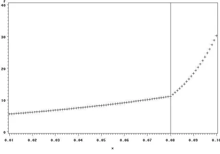
Figure 8 shows the utility function used for each monitoring site. In our entropy framework we give
more weight to sites with high utility values, that correspond to sites with greater risk of non-compliance.
Accordingly, in Figure 8 ozone design values greater than .08 ppm (80 ppb) have higher utility values since
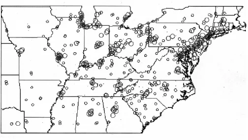
theO3NAAQS, is .08 ppm. The bubble graph (Figure 8) shows the estimated probability for an individual
site to be included in the final partition or subnetwork. This graph was calculated by simulating samples
of covariance parameter values from the posterior distribution of these parameters (using the posterior
distributions in Figures 3, 4 and 5), and then computing the best subnetwork for each sample of parameters,
using the proposed entropy-utility design approach. Monitoring sites within regions near the industrial areas
in the north east are clearly more likely to be part of the final network than sites that have low pollution.
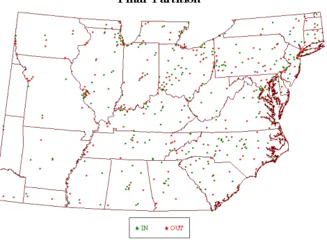
Fixing the desired number of monitoring sites to be 252, about one-half of the original network, Figure 9
shows the optimal partition using the Bayesian entropy-utility framework. This subnetwork is chosen as the
one with the maximum value (using SA) of the posterior predictive distribution for the entropy (where the
covariance parameters are updated using RJMCMC). Our approach can be used to find optimal partitions
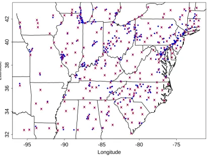
We compare our final partition (Figure 9) to a partition obtained using an alternative method proposed
by Nychka et al (1998) (Figure 10). The final network (of size 252) in Figure 10 has sites very uniformly
spaced, this is due to the assumption of stationary in the Nychka et al’s approach. Figure 9 shows that
the sites in the final partition are much more irregularly spaced, and more dense where the process is more
heterogeneous, because it is more difficult to predict ozone values at those locations. Also, due to the utility
function used in this application, the final partition in Figure 9 retains most of the sites that have high ozone
values, because those sites have higher risk of being out of compliance and our utility function gives them
more weight.
8
Conclusions
We propose a new entropy-utility design criterion based on evaluating the posterior predictive entropy
constrained by giving higher utility to maintaining sites with measurements near the ozone national ambient
air quality standard. Simulated annealing is used to select an optimal subnetwork for a fixed sample size
based on a preference relationship between entropy and utility. This approach accounts for the potential lack
of spatial stationarity in the underlying pollutant process and implements a Bayesian framework for modeling
the uncertainty about the covariance parameters. For the large-scale national ozone monitoring network,
this approach shows great promise in efficiently quantifying optimal reduced monitoring networks. Future
research will address finding optimal subnetworks relative to monitoring budget limits, evaluate networks
where a significant temporal structure might impact the choice of optimal subnetworks, and consider
non-Gaussian spatial processes.
Disclaimer
The U. S. Environmental Protection Agency’s Office of Research and Development partially collaborated in
the research described here. Although it has been reviewed by EPA and approved for publication, it does
References
Abramowitz, M. and Stegun, I. A. (1964). Handbook of Mathematical Functions. Dover, New York.
Bras, R. L. and Rodriquez-Iturbe, I. (1976). Network design for the estimation of areal mean of rainfall
events. Water Resources Research,12, 1185-1195.
Bernardo, J. M. (1979). Expected information as expected utility. Annals of Statistics,7, 686-690.
Brooks, SP and Guidici, P. (2000) MCMC Convergence Assessment via Two-Way ANOVA. Journal of
Computational and Graphical Statistics,9, p266-285.
Caselton, W. F., and Zidek, J. V. (1984). Optimal monitoring network designs. Statistics and Probability
Letters, 2, 223-227.
Cressie, N., Gotway, C. A., and Grondona, M. O. (1990). Spatial prediction from networks. Chemometrics
and Intelligent Laboratory Systems,7, 251-272.
Fuentes, M. (2001). A new high frequency kriging approach for nonstationary environmental processes.
Envirometrics,12, 469-483.
Fuentes, M. (2002). Modeling and prediction of nonstationary spatial processes. Statistical Modeling,2,
281-298.
Fuentes, M. and Smith, R. (2001). A new class of nonstationary models. Tech. report at North Carolina
State University, Institute of Statistics Mimeo Series #2534.
Gelfand, A. E. and Smith, A. F. M. (1990). Sampling-based approaches to calculating margnal densities.
Journal of the American Statistical Association, 85, 398-409.
Green, P. J. (1995). Reversible jump Markov Chain Monte Carlo computation and bayesian model
deter-mination, Biometrika,82, 711-732.
Guttorp, P., Le, N.D., Sampson, P. D., and Zidek, J. V. (1993). Using entropy in the redesign of an
envi-ronmental monitoring network. Patil, G. P., Rao, C. R. (eds.), Multivariate Environmental Statistics.
North-Holland, Amsterdam, pp 173-202.
Ko, Chun-Wa, Lee, J., and Queyranane, M. (1995). An exact algrotihm for maximum entropy sampling.
Lindley, D.V. (1956). On a measure of the information provided by an experiment. Ann. Math. Statist.
27, 986-1005.
M¨uller, P. (1999). Simulated-based optimal design. Bayesian Statistics,6, 459-474.
M¨uller, W. G. and Zimmerman, D. L. (1999). Optimal designs for variogram estimation. Environmetrics,
10, 23-27.
Nychka, D. and Saltzman, N. (1998). Design of air quality networks. In Case Studies in Environmental
Statistics,eds. D. Nychka, W. Piegorsch and L.H. Cox, Lecture Notes in Statistics number 132, Apringer
Verlag, New York, pp.51-76.
Theil, J. and Fiebig, D. G. (1984). Exploiting Continuity: Maximum Entropy Estimation of Continuous
Distributions. Cambridge, Massachusetts: Ballinger Publishing Company.
U. S. Environmental Protection Agency (2003). National Air Quality and Emissions Trends Report, 2003
Special Studies Edition. U. S. Environmental Protection Agency, Office of Air Quality Planning and
Standards, Research Triangle Park, NC 27711, EPA 454/R-03-005
Warrick,, A. W. and Myers, D. E. (1987). Optimization of sampling locations for variogram calculations.
Water Resources Research, 23, 496-500.
Wikle, C. K. and Royle, J. A. (1999). Space-time dynamic design of environmental monitoring networks.
Journal of Agricultural, Biological, and Environmental Statistics, 4, 489-507.
Yfantis, E. A., Flatman, G. T., and Behar, J. V. (1987). Efficiency of kriging estimation for square,
triangular, and hexagonal grids. Mathematical Geology,19, 183-205.
Zidek, J., Sun, W., and Le, N. (2000). Designing and integrating composite networks for monitoring
Figure 2: Location of the nodes that define the subregions of stationarity. Location of the 3 nodes: in the
i n d e x 1 2 3 D e n s i t y
0 . 0 0 0 . 0 1 0 . 0 2 0 . 0 3 0 . 0 4 0 . 0 5 0 . 0 6 0 . 0 7 0 . 0 8 0 . 0 9 0 . 1 0 0 . 1 1 0 . 1 2 0 . 1 3 0 . 1 4 0 . 1 5 0 . 1 6 0 . 1 7 0 . 1 8 0 . 1 9 0 . 2 0 0 . 2 1 0 . 2 2 0 . 2 3 0 . 2 4 0 . 2 5 0 . 2 6
y
7 8 9 1 0 1 1 1 2 1 3 1 4 1 5 1 6 1 7 1 8 1 9 2 0 2 1 2 2 2 3 2 4
Figure 3: Posterior distribution for the partial sill parameters. The indexes correspond to the three nodes in
i n d e x 1 2 3 D e n s i t y
0 . 0 0 0 . 0 1 0 . 0 2 0 . 0 3 0 . 0 4 0 . 0 5 0 . 0 6 0 . 0 7 0 . 0 8 0 . 0 9 0 . 1 0 0 . 1 1 0 . 1 2 0 . 1 3 0 . 1 4 0 . 1 5 0 . 1 6 0 . 1 7 0 . 1 8 0 . 1 9 0 . 2 0 0 . 2 1 0 . 2 2 0 . 2 3 0 . 2 4 0 . 2 5
y
2 0 3 0 4 0 5 0 6 0 7 0 8 0 9 0
i n d e x 1 2 3 D e n s i t y
0 . 0 0 . 1 0 . 2 0 . 3 0 . 4 0 . 5 0 . 6 0 . 7 0 . 8 0 . 9
y
0 1 2 3 4 5 6 7 8 9
-95
-90
-85
-80
-75
32
34
36
38
40
42
60
70
80
90
100
110
Figure 7: Utility function used for each site. Sites with observations near or above the O3 air quality
standard receive higher priority for inclusion in the final subnetwork. The horizontal axis shows the ozone
Longitude
Latitude
-95 -90 -85 -80 -75
32 34 36 38 40 42 • • • • •••• • • • • • • • • • •• •••• • • • • • • • • • • •• • ••• • • • •• • •• •• • • • • • •• •••••• • •••••• • • • • • • ••••• • • ••••• •• • • • • • • •• • • • • • •• • • • • • •••• • • ••• •• • • •• • • •• •• • • • • • • • • • • • •• • • • • •• ••• • • • •• • • • • • • • • • •• • • • • • ••• • • • • • •• • •••••• • •••• • • • • • • • • • • • • • ••• • • • • • • • • • • • •• • • • • • • • • ••••••• •• • • • •• • • • • •• • • • • • • • •• • • • • • • • • • • • • • •• • • • • • • • • • • • • • • • • •••• •• • • • • • • • •• • • • • • • • • • •••• • • •• • • • •• • • • • • •• • • • •• • • •• •• • • • • • •• • • • • • • • • • • ••• •• • • • • • •• • • • •• ••• • •• • • • • • •• • • • • •• • • • •• • • •• • • • • •• • • • • • • • • • • • ••• • • • • • • • •• • • • • • • •• • •• • •• • ••• • • • •• •• •• •• • • • • • • • • • • ••• • • •• • • • • • • • • • •• • • • • • • • • • •• ••• • • • X X X X X X X X X X X X X X X X X X X X X X X X X X X X X X X X X X X X X X X X X X X X X X X X X X X X X X X X X X X X X X X X X X X X X X X X X X X X X X X X X X X X X X X X X X X X X X X X X X X X X X X X X X X X X X X X X X X X X X X X X X X X X X X X X X X X X X X X X X X X X X X X X X X X X X X X X X X X X X X X X X X X X X X X X X X X X X X X X X X X X X X X X X X X X X X X X X X X X X X X X X X X X X X X X X X X X X X X X X X X X X X X X X X X X X X X X X X X X X X X X X X X X X X X X X
Figure 10: Final partition of size 252 using Nychka and Saltzman (1998) approach. The crosses indicate the