Numerical solution of one dimensional burgers’ equation solving with explicit FTCS method and implcit BTCS method

(1)

NUMERICAL SOLUTION OF ONE DIMENSIONAL BURGERS’ EQUATION SOLVING WITH EXPLICIT FTCS METHOD A N D IMPLCIT BTCS METHOD

NURFARHANA BINTI AZMI

(2)

NUMERICAL SOLUTION OF ONE DIMENSIONAL BURGERS’ EQUATION SOLVING WITH EXPLICIT FTCS METHOD A N D IMPLCIT BTCS METHOD

N URFARHANA BINTI AZMI

A dissertation submitted in partial fulfilment o f the requirements for the award o f the degree o f

Master o f Science

Faculty o f Science Universiti Teknologi Malaysia

(3)

lll

TO M Y BELOVED PARENTS

Azmi Bin Zahari & Syarifah Fatimah Binti Syed Mahmood

f o r always loving and supporting me

TO M Y RESPECTED SUPERVISOR

Tuan Haji Hamisan Bin Rahmat

f o r your patience and advice

(4)

iv

A C K N O W L E D G E M E N T

Alhamdulillah, thanks to Allah s.w.t. for graciously bestowing me the perseverance to undertake this study. I owe a great debt o f gratitude to many people who supported and assisted me in the preparation o f this dissertation. Million thanks and appreciation to my respected supervisor, Tuan Haji Hamisan Bin Rahmat for providing invaluable guidance and advice. N ot to forget special thanks to Dr Yeak Su Hoe for helping me a lot in programming.

I am also indebted to my parents and family. They greatly contributed in the form o f finance, energy, transport and accommodation. Next, sincere thanks to all o f

my colleagues for giving full support and help during the report preparation process.

(5)

v

A BSTR A C T

(6)

vi

A B ST R A K

(7)

C H A PTER

1

vii

LIST OF TABLE

TITLE PA G E

Comparison between explicit FTCS, implicit BTCS

with the exact solution for v = 1, h = 0.0125 and k = 1 0 5 42

Comparison between explicit FTCS, implicit BTCS

with the exact solution for v = 0.1, h = 0.0125, and k = 10 5 44

Comparison between explicit FTCS, implicit BTCS with the exact solution for v = 0.01, h = 0.0125 and k = 1 0 5 46

Comparison between explicit FTCS, implicit BTCS with the exact solution for v = 1, h = 0.0125, and k = 10 4 48

Comparison between explicit FTCS, implicit BTCS with

the exact solution for v = 0.1, h = 0.0125, and k = 10~4 50

4.6 Comparison between explicit FTCS, implicit BTCS with

(11)

xi

4.7 Comparison between explicit FTCS, implicit BTCS with the exact solution for v = 1, h = 0.05, and k = 1 0 5

at x = 0.1 until x = 0.9 55

4.8 Comparison between explicit FTCS, implicit BTCS with the exact solution for v = 1, h = 0.0125, and k = 1 0 5

at x = 0.1 until x = 0.9 57

4.9 Comparison between Explicit FTCS, Implicit BTCS with the Exact Solution for v = 1, h = 0.01, and k = 1 0 5

(12)

xii

FIG U R E NO. TITLE PAGE

1.1 Type o f fluid flows 3

3.1 Stencil for 1D Burgers’ equation for explicit FTCS 26

3.2 Position Mesh Point 26

3.3 Stencil for 1D Burgers’ equation for implicit BTCS 31

4.1 Solution with implicit BTCS method at t = 0.1, t = 0 .15,

t = 0.20and t = 0.25 for v = 1, h = 0.0125 and k = 10 5 43

4.2 Solution with implicit BTCS method for v = 1,

h = 0.0125 and k = 1 0 5 43

LIST OF FIGURES

4.3 Solution with implicit BTCS method at t = 0 .4 , t = 0 .6 , t = 0.8and t = 1.0 for v = 0.1,

(13)

xiii 4.4 4.5 4.6 4.7 4.8 4.9 4.10 4.11

Solution with implicit BTCS method for

v = 0.1, h = 0.0125 and k = 1 0 5 45

Solution with implicit BTCS method at t = 0.1, t = 0.15 , t = 0.20 and t = 0.25 for

v = 0.01, h = 0.0125 and k = 10 5 47

Solution with implicit BTCS method at t = 0 .4 0 , t = 0 .6 0 , t = 0.80 and t = 1.0

for v = 1, h = 0.0125and k = 10"4 49

v = 1 , h = 0.0125 and k = 10^ 49

Solution with implicit BTCS method

at t = 0 .40, t = 0.60, t = 0.80and t = 1.0 for

v = 0.1, h = 0.0125 and k = 10-4 51

v = 0.1, h = 0.0125 and k = 10~4 51

Solution with implicit BTCS method

at t = 0 .40, t = 0 .60, t = 0.80 and t = 1.0 for

v = 0.01, h = 0.0125 and k = 10-4 53

4.12 Solution with implicit BTCS method for

(14)

xiv

4.13 Solution with explicit FTCS, implicit BTCS and exact solution at t = 0.1 with the value o f x

as in the table 4.7 for v = 1, h = 0.05, and k = 10 5 56

as in the table 4.8 for v = 1, h = 0.0125, and k = 10 5 58

(15)

xv

L IST O F SY M B O L S

v - Kinematic viscosity

r - Stability

% - Amplification factor

(16)

xvi

L IST O F A B B R E V IA T IO N S

ODEs Ordinary Differential Equations

PDEs Partial Differential Equations

FDM Finite Difference Method

FTCS Forward-Time Central-Space

(17)

xvii

LIST OF A PPPE N D IC E S

A PPE N D IX TITLE PAGE

A1 Matlab Coding For Explicit FTCS 6 8

A2 Matlab Coding For Implicit BTCS (Main) 7 0

A3 Matlab Coding For Implicit BTCS (BC) 73

A4 Matlab Coding For Implicit BTCS (F(U)) 7 4

(18)

CHAPTER 1

IN TR O D U C TIO N

1.1 Introduction

(19)

2

1.2 Background of the Study

(20)

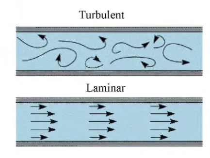
3 Turbulent d . Laminar ---- ► ---► ---► ... --► ---- ► --- ► --- ► --► --- ►

Figure 1.1: Type o f fluid flows

Furthermore in fluid dynamics, flow can also be categorized as laminar or turbulent. Based on Figure 1.1 above shows that Laminar’s flow are smoother than Turbulent’s flow which are more chaotic. A steady flow refers when the flow is independent o f time. For example, moving water in a pipe at a constant rate where it is also refers as laminar flow. Meanwhile, water moving on a surface is an example that shows an unsteady flow or called as turbulent flo w . Mathematically, turbulent flow shows that it tends to be nonlinear problem since the flow are chaotic. Many researchers are more likely to study about turbulent flow compare to laminar flow. Because o f fluid dynamics mostly referred as a nonlinear domain, thus there exist difference kinds o f nonlinear equations.

(21)

4

Besides, the existence o f Burger’s equation can be seen in the area o f applied mathematics such as in fluid mechanics, modeling dynamics, heat conduction and many more. It is named after Johannes Martinus Burgers (1895-1981). Burger’s equation can be more than one dimension, hence for this study w e only focus on one dimensional nonlinear Burger’s equations. Solving nonlinear PDEs may having difficulties in the process to get the result compare to linear PDEs which are a lot more easier. Thus for this reason, many researchers found that numerical discretization techniques can be used to solve the nonlinear PDEs can make the solution less complicated.

Fan and Li (2014) stated that although Burger's equation and the momentum o f well-known Navier-Stokes equation are similar, but the Burger’s equations are easier to be solved than the governing equations o f Navier-Stokes equation. Many studies have been done which was to compare between these two systems. Basically Burger’s is a system with time-dependent and space-dependent partial differential equations. Meanwhile there are many meshfree numerical schemes were proposed for discretization. After all each method have its own advantages and privileges when solving the problem. In fact, many researches are interested in studying the solution o f Burger’s equation and trying to solve the problems related with many type o f numerical techniques.

(22)

5

1.3 Problem Statem ent

In this area o f study, will solve the one dimensional o f Burgers’ equations with two types o f methods which are Explicit FTCS method and Implicit BTCS method. Besides, solving with Explicit FTCS can produce the solution directly. Meanwhile when solving with Implicit BTCS cannot be solved directly and need to undergo an iterative technique to get the solutions. The iterative techniques that will be used is N ew ton’s method. Since Burgers’ equation are known as a nonlinear equation, usually the number o f unknown variables is typically very large. In spite o f that, there are some problems that will appear while solving the solutions which are the stability issue and the accuracy issue. Numerical stability has to do with the behaviour o f the solution as the time step increase. Indicating that there must be some limit on the size o f the time step for there to be a solution. Apart from that, for the accuracy issue can be seen clearly when comparing the chosen solution from these two methods with the exact solution.

1.4 O bjectives o f the Study

The main purpose on doing this project is to solve the nonlinear o f one dimensional Burgers’ equations. Here are the three objectives which are:

• To formulate Burgers’ equation into discretization form.

• To investigate the consequences o f using an Explicit FTCS versus an Implicit BTCS method.

(23)

6

1.5 Scope o f the Study

The study focused on Burgers’ equation. This study only concerns on nonlinear one-dimensional Burgers’ equation. Since there are many methods that can be used to solve this problem. Thus for this study will be restricted to use Explicit FTCS method, Implicit BTCS method and N ew ton’s method. Therefore, for this case o f study MATLAB software is used for the numerical computation.

1.6 Significant o f the Study

The importance o f this study are:

• To provide numerical solution about Burgers’ equation by using Explicit FTCS and Implicit BTCS.

• To adopt the method that can solve system o f nonlinear algebraic equations in a very effective way and has great potential for large scale o f engineering problems.

1.7 D issertation O rganization

(24)

7

Chapter 1 discussed about short introduction regarding this study. Chapter 1 also includes background o f study, problem statement, objectives o f study, scope o f study and significant o f study.

Chapter 2 are about literature reviews for this study. Where lots o f information mostly in books, research paper, journals is collected. The topics that have been discussed are nonlinear equations o f PDEs, one dimensional o f Burgers’ equation, explicit FTCS method, implicit BTCS method, von Neumann stability analysis, and lastly is N ew ton’s method.

Chapter 3 illustrates the numerical discretization to solve the one dimensional Burgers’ equation. The first derivations is for explicit FTCS method. Second is implicit BTCS method. Lastly is about N ew ton’s methods.

(25)

REFERENCES

Abd-el-Malek, M.B. and El-Mansi, S.M.A. (2000). Group theoretic Methods Applied to Burgers’ Equation. Journal o f Computational and A pplied Mathematics.

115(1-2), 1-12.

Burgers, J. M. (1948) A Mathematical model illustrating the theory o f turbulence. In Advances in A pplied Mechanics, 171-199. Academic Press Inc.

Bahadir, A. R. (2003). A Fully Implicit Finite Difference Scheme for Tw o

Dimensional Burgers’ Equation. A pplied M athematics and Computation. 137 (1), 131-137.

Blanchard, P and Volchenkov, D. (2011). Random Walks and Diffusions on Graphs and D atabases: An Introduction. Berlin Heidelberg. Springer-Verlag.

Cheney, W. and Kincaid, D. (2008). Num erical M athematics and Computing. (6th ed). Brooks/Cole: The Thomson Corporation.

Chaudhry, M. H. (2008) Open-Channel Flow.. (2nd ed). N ew York, Springer Science+Business Media, LLC.

Debnath, L. (2005). Nonlinear P artial Differential Equations f o r Scientists and Engineers. (2nd ed). United States o f America: Springer.

Dehghan, M. (2003). Locally Explicit Scheme for Three-Dimensional Diffusion With a Non-Local Boundary Specification. A pplied M athematics and Computation. 138 (2-3), 489-501.

Fletcher, C. A. J. (1991). Computational Techniques f o r Fluid Dynamics 1. (2nd). Sydney Australia: Springer.

(26)

66

Fan, C.-M. and Li P.-W. (2014). Generalized Finite Difference Method for Solving Two-Dimensional Burgers’ Equations. 37th N ational Conference on Theoretical and A pplied Mechanics (37th N CTAM 2013) & The 1st

International Conference on Mechanics (1st ICM) 2013. Taiwan, 55-60.

Goyon, O. (1996). Multilevel Schemes for Solving Unsteady Equations. International Journal f o r Num erical M ethods in Fluids. 22 (10), 937-959.

Gulsu, M. and Ozis, T. (2005). Numerical Solution o f Burgers’ Equation with

Restrictive Taylor Approximation. A pplied M athematics and Computation. 171 (2), 1192-1200.

Gousidou-K. M. and Kalvouridis T. J. (2009). On the efficiency o f Newton and Broyden numerical methods in the Investigation o f the Regular Polygon Problem o f (N+1) Bodies. A pplied M athematics and Computation. 212 (1),

100- 112.

Hopf, E. (1950). The partial differential equation ut + uux = uxx. Communications on Pure and A pplied M athematics, 3: 201-230.

Hoffman, J. D. and Frankel, S. (2001). Num erical M ethods f o r Engineers and Scientists. (2nd ed). N ew York. Marcel Dekker, Inc.

Inan, B. and Bahadir, A.R. (2013). Numerical Solution o f the One-Dimensional Burgers’ Equation: Implicit and Fully Implicit exponential Finite Difference Methods Pramana. 81 (4), 547-556.

Johnson, R. W. (2016). H andbook o f Fluid Dynamics. (2nd ed). Boca Raton, CRC Press Taylor & Francis Group, LLC.

Jaluria, Y. (2012) Computer M ethods f o r Engineering with MATLAB applications. (2nd ed). Boca Raton, Taylor & Francis Group, LLC.

Logan, J. D. (2013). A pplied Mathematics. (4th ed). Canada: John W iley & Sons, Inc., Hoboken N ew Jersey.

Liu, T.-P. (2000). On Shock Wave Theory. Taiwanese Journal O fMathematics Vol. 4: 9-20.

Li, J. and Yang, Z. (2013). The von Neumann Analysis and Modified Equation

Approach for Finite Difference Schemes. A pplied M athematics and Computation. 225, 610-621.

Mohanty, A. K. (2006). Fluid M echanics. (2nd ed). N ew Delhi: Asoke K.Ghosh.

(27)

67

Mellodge, P. (2016). A P ractical Approach to D ynam ical Systems f o r Engineers. Woodhead, Elsevier Ltd.

Mishra, C. (2016). A N ew Stability Result for the Modified Craig-Sneyd Scheme Applied to Two-Dimensional Convection Diffusion Equations with Mixed Derivatives. A pplied M athematics and Computation. 285, 41-50.

Noye, B. J. et. al (1989). A Comparative Study o f Finite Difference Methods for Solving The One-Dimensional Transport Equation with an Initial-Boundary Value Discontinuity. Computers Math. A pplic.(20), 67-82.

Noye, B. J. and Dehghan, M. (1994). Explicit solution o f Two-dimensional Diffusion Subject to Specification o f Mass. M athematics and Computers in Simulation. 37 (1), 37-45.

Ozisik, M. N. (1994). Finite Difference M ethods in H eat Transfer. United States o f America:CRC Press.

Pinchover, Y. and Rubinstein, J. (2005). An Introduction to P artial Differential Equations .United Kingdom, Cambridge University Press.

Pletcher, R. H. et. al. (2013) Computational Fluid M echanics and H eat Transfer. (3rd ed). Boca Raton, Taylor & Francis Group, LLC.

Remani, C. (2013). Num erical M ethods f o r Solving Systems o f Nonlinear Equations. Canada, Lakehead University.

Ramos, H. and Moteiro, M. T. T. (2016). A new Aproach Based on the N ew ton’s Method to Solve Systems on nonlinear equations. Journal o f Computational and A pplied Mathematics. 318 (2017), 3-13.

Rivera-Gallego, W. (2003). Stability Analysis o f Numerical Boundary Conditions in Domain Decomposition Algorithms. A pplied M athematics and Computation.

137 (2-3.), 375-385.

Sen, S., Srinivas, C.V., Baskaran, R., and Venkatraman, B. (2015). Numerical

Simulation o f The Transport o f a Radionuclide Chain in a Rock Medium. Journal o f environmental Radioactivity. 141, 115-122.