Int. J. Advance Soft Compu. Appl, Vol. 9, No. 3, November 2017 ISSN 2074-8523
Single Class Classifier Using FMCD-Based
Non-Metric Distance for Timber Defect
Detection
1Ummi Raba’ah Hashim, 2Siti Zaiton Mohd Hashim, 1Azah Kamilah Muda,
1Kasturi Kanchymalay, 1Intan Ermahani Abdul Jalil, 3Muhammad Hakim
Othman
1Computational Intelligence and Technologies Lab, Faculty of Information and Communication Technology Universiti Teknikal Malaysia Melaka (UTeM), Melaka, Malaysia
e-mail: [email protected]
2Faculty of Computing, Universiti Teknologi Malaysia (UTM), Johor, Malaysia [email protected]
3Hasro Group of Companies [email protected]
Abstract
Keywords: automated vision inspection, Mahalanobis distance, one class classifier, surface defect, timber image, timber defect detection, wood inspection.
1 Introduction
Automated inspection of timber defect has shown to be of great importance in the wood industry. Due to the decreasing forest resources and increasing cost of timber, the application of automated vision inspection is seen as a solution to optimise resources and save production cost, while maintaining the output of products with reliable quality. According to Kline [1], automated timber inspection was found to be more accurate and consistent than manual inspection. Conventional inspection process is seen as not to be efficient enough in optimizing timber resources, thus, the timber industries must innovate to survive in the competitive market [1].
A study has shown that human error in timber inspection resulted in 22% rejected parts which reduced the overall yield from 63.5% to 47.4% [2]. Similarly, Huber [3] claimed that the performance of human operators in locating and identifying surface defects is only about 68%. They highlighted that by applying automated inspection process, an improved yield could be obtained because obviously machine could not be affected by human weakness factors such as tiredness, boredom and inconsistencies. Kim and Koivo [4] also agreed that automated inspection could overcome the problem of suboptimal and inconsistencies of human operators judgement due to variability of defect characteristics itself. Buehlmann and Thomas [5] further concluded that improvement in 25% detection accuracy could increase yield by 5.3%, which could contribute to significant cost saving for an average sized rough mill. Since many research found that automated vision inspection is more effective than human operators, it is pertinent to apply it in timber industry to increase timber yield and improve the production quality.
Various classification method has been proposed for automatic timber defect detection as discussed in [6]. Despite having varied classification performance, it is very difficult to compare between studies because obviously each study has employed different image acquisition setting, species, types of defects and even if a similar set of features were used, the extraction parameters were dissimilar to each other. However, it is worth to note that most classifiers used were supervised classifiers [7–11] and only a few applied unsupervised methods [12–14]. This is due to the limitation of unsupervised classification in identifying defects type despite having good detection performance.
201 Single Class Classifier Using FMCD-Based
previous studies the samples used are limited to only one type of species [9,11,15]. It will be difficult to bring the outcome of a particular research to the industry if the model trained is tuned to fit only one type of species, when in reality, timber industries process multiple species at a time. However, there are some efforts reported using multiple species [7,8] but their works were confined to supervised method requiring sufficient samples.
2 Problem Background
Distribution of samples in timber inspection studies is often imbalanced. This is due to the fact that some defect types are scarce on certain timber species while being common to others. Previous studies on timber defect detection have mostly focused on samples from single timber species and supervised learning method. This is understandable, since it is difficult to obtain sufficient samples representing all types of defects for all kinds of timber species. The easiest workaround back then was to experiment on all types of defects focusing on a single species or experiment on a single type of defect only. Furthermore, the choice of supervised learning often demonstrates good performance when the training and testing data are well sampled. Nonetheless, in this way, it seems unfeasible to bring the research outcome to the industry where multiple timber species are being processed in daily production. We could not expect the industry to re-train their model for every timber species, let alone finding samples of all defect types for that particular species.
Additionally, non-defect samples have varied appearance in grain and colour over different species. However, it is known that defect characteristics are almost similar across species. Therefore, this enables us to draw a certain insight towards finding appropriate classification method which could cater to the incompleteness or unavailability of defect samples, moving away from the supervised learning approach. In this light, we propose a timber defect detection approach based on the concept of outlier detection, where defects will be detected or classified as the timber being scanned under the visual inspection system regardless of timber species. In this concept, defects will be treated as outlier and clear-wood as representative of the sample distribution. This concept is notable and considered to be a promising approach in visual inspection where defect samples are unavailable [16]. However, in the case where sufficient prior knowledge is available, supervised classification is still recommended as it often provides good performance [16].
the approach of one class learning is thought to be effective in a certain context depending on the problem domain, extensive knowledge about the learning algorithm and problem domain is needed as the algorithm will be modified according to the problem concerned [17]. The one class learning approach is very suitable for problems that require samples from only one class (clear-wood class), hence, practical in defect detection as in outlier detection concept. Due to the nature of timber defect detection problem, using one class learning, with clear-wood samples treated as representative of the distribution seems worth to be investigated.
Fig.1:Research solutions to the problem of classification of imbalanced data [17]
3 Method
3.1 Distance-based one class classifier (OCC)
203 Single Class Classifier Using FMCD-Based
rejected. This is one of the algorithm-level approaches in handling imbalanced data where defect samples are scarce and limited in availability [17]. This is often due to the lack of occurrence for the defect cases and difficulties in getting the samples. The difficulties in certain domain could be caused by higher cost, unavailability and also risk in acquiring the samples. In this case, defect samples discriminating the outlier from the target class is difficult to be defined. Therefore, OCC aims to represent the normal cases with a domain descriptor so that it would be able to detect abnormality and reject outliers by means of proximity function. In timber defect detection, the classifier’s task is to identify and assign normal or defect label to the input image. In contrast to supervised classification, it only needs clear wood samples for training, using a distance-based measure and a predefined threshold for classification. There are several types of OCC [18]:
Based on neighbourhood: A domain descriptor can be built using the neighbourhood relations to some representation objects. Such objects are chosen as the ones which have relatively many close (as judged by dissimilarities) neighbours.
Based on proximity to distribution average estimate: One of the simplest ways to describe a class relies on the proximity to the average representative. If samples are described as vectors in a feature space, then the mean vector plays the role of average representative. To identify multivariate outlier, distance from each sample and distribution’s average is calculated. An outlier will be detected as a point having distance larger than a pre-set cut-off.
Based on dissimilarity space (boundary): A dissimilarity space is defined by a space which contains samples from the class of interest. Samples are considered outliers if they are larger than the predefined dissimilarity measures. If the dissimilarity measure is a metric, then all samples are contained in a prism, bounded from below by a hyper plane and bounded from above by the largest dissimilarities.
Based on probability distribution function: Probabilistic approach utilises the kernel function to estimate general distribution of samples, establishing decision boundaries (determined by the probability distribution) and rejecting samples lying in the regions of low density by examining data likelihood.
Similarity or distance measures play an important role as proximity function in OCC based on distribution average estimate. Choosing a distance metric is highly problem dependent and will determine the success or failure of the proposed learning approach [19]. There are two types of distance measures, namely metric and non-metric distance. Metric distance is based on Euclidean distance where data measured must be standardized to a similar scale as to obey the rules of triangular inequality. It assumes that each feature is independent from others and equally important [19]. However, in real multi-dimensional problem, similarity judgement is based on different weight for different dimension.
-In our study, the measurement of the proposed statistical texture features is of different scaling, hence, different weight for every feature. Furthermore, metric distance was claimed to be not effective for multivariate outlier detection as the distance between samples in high dimensional space is so similar that none of the samples can be treated as outlier [20]. Kou [20] further concluded that non-metric distance has many advantages over metric distance in handling multivariate data. For example, metric distance treats each feature as equally important, while non-metric distance such as Mahalanobis distance will automatically account for the scaling of unstandardized data [20]. Weinshall et al. [21] also emphasized that outlier detection method must implement non-metric distance that violates the triangle inequality. Pekalska et al. [22] further agreed that non-metric distance is more useful and informative in statistical learning involving multidimensional data.
Therefore, for our work, we will employ a non-metric distance which is based on Mahalanobis formulation. Mahalanobis distance was introduced by Mahalanobis [23] and since then has been used in many domains including on outlier detection problem [24]. Mahalanobis distance is a scale-invariant distance measure between two data points in a multi-dimensional space. Since it is a non-metric distance, it accounts for unequal variances as well as correlations between features [19,24]. Therefore it is an appropriate distance measure when it comes to handling multiple features of unequal scale. Mahalanobis-based classifier falls under the category of distance-based non-parametric classifiers. It is under the same group as template matching and k-nearest neighbour classifier, where there is no assumption of model. This is contrasting to parametric or semi-parametric classifiers such as artificial neural network, support vector machine and linear discriminant analysis, where data is assumed to be represented by a distribution model. Mahalanobis distance can be defined as follows:
Mahalanobis Distance, D(x) = (1)
Where,
205 Single Class Classifier Using FMCD-Based
μ = mean vector of the feature space distribution Σ = covariance of the feature space distribution
In our case, as a sample image is scanned, the image will be subdivided into non-overlapping rectangular sub-images. Feature space distribution is generated from texture features extracted over all sub-images of a sample image. When applied to timber defect detection, an underlying assumption is that the mean vector represents optimal defect-free condition. This is based on the fact that defect area is approximately ranging from 5 to 25 percent for each piece of timber. Distance between all sub-images and distribution centroid will be calculated using Eq. 1. Distance space calculated using Mahalanobis distance can be approximated following a chi-square distribution where p is the number of features or dimensions [25]. Therefore, finding multivariate outlier in Mahalanobis distance space can be done by setting a cut-off value to a corresponding chi-square distribution χ2 , for example 98% quantile, subsequently treating the points with
distance larger than the cut-off value as defect.
However, using mean as multivariate distribution estimator has several disadvantages and it was claimed as a non-reliable measure for outlier detection [25] . Mean value is considered to be sensitive to extreme data deviating from the main distribution [25]. Furthermore, classical mean as estimator is subject to the problems of masking (false positive) and swamping (false negative) where outliers do not necessarily show large distance [26]. Hardin and Rocke [27] suggested that these problems could be overcome by using robust estimates which are less affected by outliers. Therefore, Mahalanobis distances need to be calculated from robust distribution estimate in order to provide reliable measures for defect (outlier) detection. Many robust estimators have been introduced in the literature. According to Filzmoser [25], the minimum covariance determinant (MCD) estimator is most frequently practiced, for having a computationally fast algorithm. The next section will explain the Fast Minimum Covariance Determinant algorithm in producing robust estimator of multivariate location. We consider the FMCD algorithm as an extension or improvement over the proposed Mahalanobis distance based classifier in increasing the detection accuracy of our timber defect detection problem.
3.2 Fast minimum covariance determinant as robust estimator
considered as the minimum number of samples which must not be treated as outlier. According to Hardin and Rocke [27] h is normally set to be higher than its highest possible breakdown which is,
, where p = number of dimension (2)
Consequently, the mean and covariance from the subset having the lowest covariance determinant (most concentrated distribution) will be considered as robust distribution estimator, hence used in our Mahalanobis classifier. In our case, MCD estimator will replace the classical mean and covariance in the Mahalanobis distance formula with the robust mean (location estimate) and robust covariance matrix (scatter estimate) of samples subset that have a minimum covariance matrix determinant.
(3)
Where,
(4)
(5)
(6)
Therefore, Robust Mahalanobis Distance, RMD is formulated by,
(7)
From Eq. 4, the original MCD estimator is very difficult to compute, as it needs to evaluate all subset Q of size h. A more efficient algorithm, called Fast Minimum Covariance Determinant (FMCD) algorithm was introduced to solve the computation problem with C-step (concentration) as the key component [28]. The FMCD algorithm [26,28] is explained as follows :
Consider dataset X and subset H1:
(8)
Compute mean and covariance matrix of subset H1:
207 Single Class Classifier Using FMCD-Based
(10)
If , define the relative distance,
(11)
Now take such that
(12)
Taken from the following ordered distances,
(13)
Then, we shall compute and . After that, we compare the determinant,
(14)
with equality if and only if and . If , the C-step yields a with lower determinant, thus is more concentrated than .
C-step is then iterated until or . MCD
solution can be approximated by taking a few initial choices of H1 , applying
C-steps to each and finally keeping the lowest determinant as the solution.
The initial subset, H1 is constructed by drawing a random subset J of size (p+1),
subsequently computing and . If , J can be extended by adding another samples until . Then , compute and sort the distance,
(15)
The initial H1 subset is then consists of h samples with smallest . This method is
claimed to draw a better initial subsets with higher probability of outlier-free subsets than taking random subsets of size h [28].
3.3 Overview of proposed method
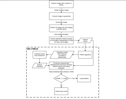
sample distribution. The MCD is computed using Fast-Minimum Covariance Determinant (FMCD) algorithm for faster convergence, ensuring fast detection of timber defect. We call the proposed classifier as Mahalanobian Classifier based on Robust FMCD (MC-FMCD).
As shown in Fig. 2, timber surface images acquired using an optical sensor, were converted into greyscale and divided into non-overlapping rectangular regions of 60 x 60 pixels. 15 statistical texture features based on the orientation independent Grey Level Dependence Matrix (GLDM) [29] were then extracted from each region to form a feature vector representing the regions for the whole timber. The FMCD algorithm was then employed where the mean and covariance of the distribution subset from the feature vector with minimum covariance determinant were used to represent the distribution centroid. Defects were then detected based on proximity measurement between each sample in the feature vector and the robust distribution centroid. The proximity measurement employed was based on robust Mahalanobis Distance, where a distance larger than the pre-set cut off value of a corresponding chi-square distribution would be treated as defect. All equations related to MC-FMCD can be referred to in Eq.7 to Eq. 15.
Acquire Image from a piece of timber
Division of image into sub-images of 60x60 pixels Convert image to greyscale
Extract statistcal features based on orientation independent GLDM
for each sub-images
FMCD algorithm Feature
Vector
Samples subset with minimum
covariance determinant Calculate mean
and covariance
Robust estimator
Proximity measurement (Mahalanobis distance) between
feature values and robust estimator
If RMD > χ2 cutoff
Robust Mahalanobis Distance, RMD
Label=defect
Label=clear wood Sub-images/samples Timber surface image
Greyscale image
No
Yes
MC-FMCD
209 Single Class Classifier Using FMCD-Based
4
Experimental Results and Discussion
4.1 Experimental setting
In this study, we used the Malaysian timber defect database from the Computational Intelligence and Technologies Lab, Universiti Teknikal Malaysia Melaka [30]. The image database contains 8 types of natural defect commonly found on the surface of timber from four species which are Merbau, Rubberwood, KSK and Meranti. We constructed our experimental datasets by combining sub-images of clear wood and defects from the database with defect ratio between 5-25% to simulate the original timber length. The ratio was set based on suggestions from industry expert. Each dataset contained about 720 samples of 60 x 60 pixels to simulate a timber piece with a size of 10 feet x 4 inches (approximately 1200 x 360 pixels). There were 45 datasets for each timber species with various combinations of clear wood and defects at various defect ratios. The alpha value for FMCD was set to 0.75, which means that 75% of the samples were used as the subset for finding the minimum covariance determinant. The chi-square cut-off value was set to 0.99, .
4.2 Performance measurement indices
4.2.1 Precision, recall and F measure to measure detection performance
In this study, defect images contributed to lower number of samples compared to clear wood samples. This is not uncommon, especially in secondary wood industry where the rejection rate or percentage of raw material defect often ranges from 5% to 10%. The sub images of collected samples were expected to be skewed where clear wood area is higher than defect area. Therefore, the number of positive samples (defect) is much smaller than the number of negative samples (clear wood). In this case, one useful evaluation metric is called precision/recall. For skewed classes, precision/recall gives us a more direct insight into how the learning algorithm is doing and often, is a much better way to evaluate our learning algorithm than looking at classification error and accuracy [31]. Precision and recall measures will give us a better sense on how well our classifier is doing [31]. Brownlee [32] agreed that in an imbalanced class situation, accuracy measure can be misleading because if a model is able to predict the majority class over all predictions, it can achieve high accuracy even if the minority class is not predicted well. Precision, recall and F measure are defined as follows:
(17)
(18)
Precision and recall provides a complementary measure. We may want to have a balanced precision and recall depending on our problem domain. To produce a single performance measure on precision and recall, we used F measure [31,33,34]. F measure is a weighted harmonic mean of precision and recall [33]. It is a combined measure to evaluate the trade-off between precision and recall. The value of F measure ranges from 0 to 1 where 1 is considered to be a perfect score. F measure may also provide a reasonable rank ordering of different classifier or different parameters used in classification. For very skewed classes, a classifier with high precision and recall indicates that the classifier chosen is performing well [31].
4.2.2 Over detection and under detection errors
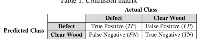
Over detection and under detection errors are among the suggested measure to assess the quality of segmentation when manual reference exists [35]. Over detection error can be defined as over segmented area with regards to automated segmentation produced, while under detection error can be defined as under segmented area over an actual segmentation. As non-segmenting approach is employed in our work, errors are measured through the establishment of correspondence between manually labelled sub-images and predicted sub-images. This is equivalent to producing a confusion matrix where four measures are calculated as in Table 1.
Table 1: Confusion matrix
Actual Class
Defect Clear Wood
Predicted Class Defect True Positive (TP) False Positive (FP) Clear Wood False Negative (FN) True Negative (TN)
Then, over detection (OD) and under detection (UD) errors are defined as:
(19)
211 Single Class Classifier Using FMCD-Based
OD can be defined as over detected defect (clear wood detected as defect), while UD can be defined as undetected defect (defect detected as clear wood).
4.3 Experimental results
In this section, we will present the experimental results to measure the detection performance of the proposed approach. The results are presented in three dimensions with the first one being measured across timber species to evaluate the performance consistency of the proposed approach over multiple timber species. The second detection performance result is presented by defect types to identify the detection performance of each individual type of defects. This is followed by performance comparison between classic MD and robust MD to prove that the robust MD provides better defect detection due to its robustness in detecting outlier.
4.3.1 Detection performance by timber species
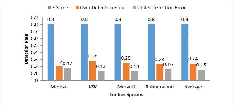
Fig. 3 summarizes the detection performance (average F score, average OD and UD error) of MC-FMCD over all timber species; Merbau, KSK, Meranti and Rubberwood.
From Fig. 3, it is apparent that MC-FMCD performs satisfactorily well over multiple timber species with small OD and UD errors and an F score of about 0.8 for all species. Additionally, OD error seems to be mostly higher than UD error across all species. Over detected defect samples are seen to contribute to most of the detection error compared to under detected samples. This confirms that despite minor confusion with clear wood, defects could still be detected well and the slight confusion with clear wood might be due to the variability in the clear wood appearance.
4.3.2 Detection performance by defect types
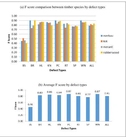
Further look into the performance summary as in Fig. 4 indicates a consistent performance over all defect types across multiple species with all defect types showing good performance except for blue stain which consistently performs poorly for all timber species.
(a) F score comparison between timber species by defect types
(b) Average F score by defect types
Fig. 4: Average detection performance by defect types across timber species (a) F score comparison between timber species by defect types (b) Average F score by
213 Single Class Classifier Using FMCD-Based
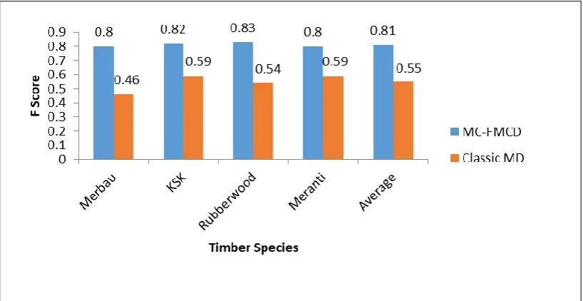
4.3.3 Detection performance between MC-FMCD and MD
Lastly, Fig. 5 summarizes the detection performance comparison between MC-FMCD and classic MD over multiple timber species and also the overall average performance. It can be observed that MC-FMCD performs better than classic MD consistently across timber species and on average. We also conducted paired samples T-Test to test the statistical significance of the performance improvement (average F score) between MC-FMCD and classic MD. As a result, there is a significant effect in detection performance, t(44)=8.29, p<0.001, with MC-FMCD (mean F score=0.81) performing significantly better than classic MD (mean F score =0.55).
Fig. 5: Average detection performance between MC-FMCD and classic MD
4.4 Discussion
detection performance for blue stain could be improved since the blue stain could be visually distinguished over clear wood by its bluish appearance.
The experimental result shows that over detection error is mostly higher than under detection error suggesting that defects are mostly detectable despite minor confusion with clear wood. This indicates that the proposed approach combined with the statistical texture feature set provides an appropriate representation towards successful detection that can be generalized well enough for many types of defects. Nevertheless, for future research, we suggest further improvementon the detection procedures to reduce over detection error in order to avoid over rejected parts in future industrial application.
The proposed MC-FMCD has also demonstrated superior detection accuracy compared to classic MD, and is proven by a statistically significant improvement in average F score over multiple timber species as well as in the average value. This suggests that the robust estimator provided by the FMCD algorithm works really well in improving the detection of outlier in the samples, thus increasing defect detection accuracy.
5
Conclusion
This paper discusses the proposed timber defect detection using MC-FMCD and the evaluation of the approach on simulated dataset. Experiments are first conducted on simulated datasets with multiple imbalance ratios covering all defect types either individually or combined. Results from the experiments demonstrate that MC-FMCD which is based on robust estimator derived from FMCD is useful in contributing to acceptable defect detection accuracy over all defect types (except for blue stain) and consistently across multiple timber species. The poor performance on detecting blue stain is due to blue stain having close similarity of texture characteristics with clear wood. Additionally, MC-FMCD performs significantly better than classic MD in detecting defects.
ACKNOWLEDGEMENT
The authors wish to thank Hasro Malaysia, Teras Puncak and Elegant Success (wood product manufacturers in Malaysia) for providing invaluable feedback and consultation. The researcher is sponsored by Ministry of Education, Malaysia, Universiti Teknikal Malaysia Melaka and Universiti Teknologi Malaysia.
References
[1] D. Kline, C. Surak, P.A. Araman (2003). Automated hardwood lumber grading utilizing a multiple sensor machine vision technology. Computer & Electronic in Agriculture, 41(1-3), 139–155.
215 Single Class Classifier Using FMCD-Based
197–203.
[3] H.A. Huber, C.W. Mcmillin, J.P. Mckinney(1994) Lumber defect detection abilities of furniture rough mill employees. Forest Product Journal, 35(11), 79–82.
[4] C.W. Kim, A.J. Koivo (1994). Hierarchical classification of surface defects on dusty wood boards. Pattern Recognition Letter, 15(7), 713–721.
[5] U. Buehlmann, R.E. Thomas (2006). Relationship between lumber yield and board marker accuracy in rip-first rough mills. Holz Als Roh- Und Werkstoff, 65(1), 43–48.
[6] U.R. Hashim, S.Z. Hashim, A.K. Muda (2015), Automated Vision Inspection of Timber Surface Defect: A Review. Jurnal Teknologi, 77(20),127–135. [7] Y. Xie, J. Wang (2015). Study on the identification of the wood surface
defects based on texture features. Optik - Int. J. Light Electron Optics (2015). [8] S.M. Lee, P. Araman (2009). Automated grading, upgrading, and cuttings prediction of surfaced dry hardwood lumber. In Proc. 6th Int. Symp. Image Signal Processing Analysis (pp. 371–376).
[9] P.A. Estevez, C.A. Perez, E. Goles (2003). Genetic input selection to a neural classifier for defect classification of radiata pine boards. Forest Product Journal. , 53, 87–94.
[10] A. Ziadi, F. Ntawiniga, X. Maldague(2007). Neural networks for color image segmentation: Application to sapwood assessment. In Canadian Conf. Electrical & Computer Engineering (pp. 417–420). IEEE.
[11] A. Rinnhofer, G. Jakob, E. Deutschl, W. Benesova, J.P. Andreu, G. Parziale (2005). A multi-sensor system for texture based high-speed hardwood lumber inspection. In Electron. Imaging 2005, International Society for Optics and Photonics (pp. 34–43).
[12] O. Silven, M. Niskanen, H. Kauppinen(2003). Wood inspection with non-supervised clustering. Machine Vision Application, 13(5-6), 275–285.
[13]M. Niskanen (2001). Experiments with SOM based inspection of wood. In Int. Conf. Qual. Control by Artif. Vis. (pp. 311–316).
[14] M. Niskanen, O. Silven, H. Kauppinen(2001) Color and Texture Based Wood Inspection with Non-Supervised Clustering. In Proc. Scand. Conf. Image Anal.(pp. 336–342).
[15] G.A. Ruz, P.A. Estevez, C.A. Perez (2005) A neurofuzzy color image segmentation method for wood surface defect detection. Forest Product Journal, 55(4), 52–58.
[16] X. Xie (2008). A Review of Recent Advances in Surface Defect Detection using Texture analysis Techniques. Electron. Lett. Comput. Vis. Image Anal., 7(3), 1–22.
[17] Y. Sun, A.K.C. Wong, M.S. Kamel(2009). Classification of Imbalanced Data: a Review. Int. J. Pattern Recognit. Artif. Intell., 23(4), 687–719.
[18] E. Pekalska (2005) Dissimilarity representations in pattern recognition.
for data clustering and classification. Pattern Recognit.,41(12), 3600–3612. [20] Y. Kou (2006) Abnormal Pattern Recognition in Spatial Data. Virginia
Polytechnic Institute and State University.
[21] D. Weinshall, D. Jacobs, Y. Gdalyahu (1999), Classification in non-metric spaces. Adv. Neural Inf. Process. Syst., 838–844.
[22] E. Pekalska, A. Harol, R.P.W. Duin, B. Spillmann, H. Bunke(2006). Non-Euclidean or Non-metric Measures Can Be Informative. In Struct. Syntactic, Stat. Pattern Recognit.(pp. 871–880)
[23] P.C. Mahalanobis(1936). On the generalised distance in statistics. Proc. Natl. Inst. Sci. India, 2(1), 49–55.
[24] R. De Maesschalck, D.J. Rimbaud, D.L. Massart (2000) The Mahalanobis distance, Chemom. Intell. Lab. Syst., 50(1), 1–18.
[25] P. Filzmoser, A multivariate outlier detection method, 2004. http://computerwranglers.com/com531/handouts/mahalanobis.pdf (accessed November 6, 2014).
[26] P.J. Rousseeuw, K. Van Driessen (1999). A fast algorithm for the minimum covariance determinant estimator. 41(3), 212–223.
[27] J. Hardin, D.M. Rocke (2005). The Distribution of Robust Distances. J. Comput. Graph. Stat., 14(4), 928–946.
[28] M. Hubert, M. Debruyne(2010). Minimum covariance determinant, Wiley Interdiscip. Rev. Comput. Stat., 2(1), 36–43.
[29] U.R. Hashim, S.Z. Hashim, A.K. Muda(2016). Performance evaluation of multivariate texture descriptor for classification of timber defect. J. Light Electron Opt., 127(15), 6071–6080.
[30] U.R. Hashim, S.Z. Hashim, A.K. Muda(2015), Image Collection for Non-Segmenting Approach of Timber Surface Defect Detection, Int. J. Adv. Soft Comput. Its Appl., 7(1), 15–34.
[31] Y.A. Ng (2011). Machine Learning System Design : Error Metrics for Skewed Classes. Stanford Univ.
[32] J. Brownlee (2014). Classification Accuracy is Not Enough: More Performance Measures You Can Use. Mach. Learn. Mastery. http://machinelearningmastery.com/classification-accuracy-is-not-enough-more-performance-measures-you-can-use/ (accessed March 21, 2014).
[33] M. Christopher, R. Prabhakar(2008). Information Storage and Retrieval : Evaluation.
[34] J. Arguello(2012). Predictive Analysis : Evaluation and Experimentation. [35] M. Petrou, P.G. Sevilla(2006). Image Processing : Dealing with Texture.