www.ijiset.com
Root Finding With Some Engineering Applications
Tekle Gemechu
Department of mathematics, Adama Science and Technology University, Adama, Ethiopia
Abstract
In this article, derivative estimations up to the third order (in root finding, some new initiatives) are applied in Taylor’s approximation of a nonlinear function / equation to achieve efficient iterative methods. Competent methods of higher orders for solving simple roots of nonlinear equations, which improve convergence of some basic existing methods, are investigated. We shall offer several examples for test of efficiency and convergence analyses, in C++. We also provide some examples of engineering applications of root finding. Graphical demonstrations are using matlab basic tools.
Keywords: Derivativeestimations, applications, Taylor’s approximation, iterative methods, simple root
1. Introduction
Nonlinear equations emerge in most science and engineering models. For example, in circuit analysis, analysis of state equations for a real gas, mechanical motions / oscillations, weather forecasting, in optimization and many other fields of engineering. Nonlinear problems are difficult to solve but they occur naturally.
Some existing iterative root finding methods such as the secant method needs more than one initial guesses. And others may contain higher derivatives [1, 2, 3, 10]. In this research, we substitute the higher derivative
f
'
'
'
in termsof
f
,
f
'
andf
'
'
to minimize the number of function evaluations which can also help us develop new one-point fixed point iterative algorithms / models from the third order Taylor’s approximation / interpolation of a nonlinear model / equationf
(
x
)
. These derivative estimations are not the actual function evaluation but a kind of replacement (to reduce algorithm complexity), which we are to propose only in root finding. This is our main success.This manuscript consists of 1) introduction and starting reviews 2) construction methods 3) Analysis 4) test equations and results 5) applications 6) conclusion and recommendation 7) references.
1.2. Some starting / Review points
Let us begin with the Taylor’s approximation of
)
(
x
f
about an approximate rootr
=
x
o+
h
,with x0 an initial guess for a root r of
f
(
x
)
andh
is too small.... ) ( '' ' 6 / 1 ) ( '' 2 / 1 ) ( ' ) ( )
( + = + + 2 + 3 +
o o
o o
o h f x hf x h f x hf x
x
f (1)
The linear approximation
f
(
x
o)
+
hf
'
(
x
o)
≈
0
gives the Newton’s method [2, 3, 4]n
k
x
f
x
f
x
x
k k k
k
:
0
,
1
,...,
)
(
'
)
(
1
=
−
=
+ (2)
If we consider quadratic
interpolation (approximation) of
f
(
x
)
as0
)
(
''
2
/
1
)
(
'
)
(
)
(
x
o+
h
=
f
x
o+
hf
x
o+
h
2f
x
o≈
f
,
then we obtain Halley’s method (3), Chebyshev’s method (4), the extended Newton’s method (5) and Euler’s method (6) below, [2, 3, 5, 6, 14].
)
('
'
)
(
2
/
1
)]
('
[
)
('
)
(
2 1k k k
k k k
k
x
f
x
f
x
f
x
f
x
f
x
x
−
−
=
+ (3)
3 2
1
)] (' [
) (' ' )] ( [ 2 / 1 ) ('
) (
k k k k
k k k
x f
x f x f
x f
x f x
x+ = − − (4)
].
)
(
''
)
('
'
)
(
2
)]
(
'
[
)
(
''
)
(
'
[
)
(
2
x
f
x
f
x
f
x
f
x
f
x
f
x
x
=
−
±
−
www.ijiset.com
.
)
(
'
)
(
)
(
,
)
(
'
)
(
''
)
(
)
(
,
)
(
2
1
1
)
(
2
)
(
x
f
x
f
x
G
x
f
x
f
x
G
x
p
x
p
x
G
x
x
=
=
−
+
−
=
ϕ
[7] (6)
In addition, Halley’s method (3) and Chebyshev’s method (4) can be obtained applying Newton’s method for solving
simple roots of 1/2
)]
(
'
[
)
(
)
(
x
f
x
f
x
u
=
[3].And one can alsoobtain (7) if
)]
(
'
[
)
(
)
(
x
f
x
f
x
u
=
and then Newton’s methodis applied [4].
)
('
'
)
(
)]
('
[
)
('
)
(
)
(
2 k k k k k k kx
f
x
f
x
f
x
f
x
f
x
x
−
−
=
φ
. ( 7)Note that (2) & (7) are second order and (3), (4), (5) & (6) are cubic order convergent. The following, our finding, is based on some ideas used in the above discussions.
2. New Methods by Derivative Estimations
In this section, we apply derivative estimation (substitution) technique (a very new idea) in the third order Taylor’s (interpolation) approximation to construct new one-point iterative models.
We shall apply a technique of replacement of a higher
derivative (here
f
'
''
=
F
(
f
,
f
'
,
f
''
)
by lower derivatives (in terms off
,
f
'
andf
'
'
). This will reduce the cost of function evaluations and may increase efficiencyindex
(
e
=
p
1/f).
The higher derivative estimations we are proposing isf
'
'
'
=
F
(
f
,
f
'
,
f
'
'
)
.Some of which we shall prove in our future works. Now to derive our new algorithms, let
.0
)
('
''
6
/
1
)
('
'
2
/
1
)
('
)
(
)
(
x
o+
h
=
f
x
o+
hf
x
o+
h
2f
x
o+
h
3f
x
o≈
f
(8))'
'
2
/
1
(
)'
''
6
/
1
'
(
''
'
6
/
1
'
)
8
(
2 2 3f
h
f
f
h
f
h
f
h
hf
+
−
=
+
=
+
⇒
. (9)
Using 2
)
2'
(
f
f
h
=
−
in (9), we obtain an iterativealgorithm (10)
.
)
('
''
)]
(
[
)]
('
[
6
)
('
'
)]
(
[
)]
('
)[
(
2
3
)
(
3 22 2 1 n n n n n n n n n n
x
f
x
f
x
f
x
f
x
f
x
f
x
f
x
x
x
+
+
−
=
=
+
ϕ
((10)Inserting
'
)
''
(
''
'
2f
f
f
=
,f
f
f
f
'
''
=
'
''
andf
'
''
=
−
f
''
into (10), algorithms (11), (13) and (15) below can be obtained.
.
)
('
)]
('
'
)
(
[
)]
('
[
6
)
('
'
)]
(
[
)]
('
)[
(
2
3
)
(
2 3 2 2 1 n n n n n n n n n n nx
f
x
f
x
f
x
f
x
f
x
f
x
f
x
f
x
x
x
+
+
−
=
=
+
ξ
(11).
)
)]
('
[
)]
('
'
)
(
[
6
/
1
1
))(
('
'
)
(
)]
('
[
2
(
)
('
)
(
2
4 2 2 n n n n n n n n nx
f
x
f
x
f
x
f
x
f
x
f
x
f
x
f
x
+
−
−
=
(12))
('
'
)
('
)
(
)]
('
[
6
)
('
'
)]
(
[
)]
('
)[
(
2
3
)
(
3 2 2 1 n n n n n n n n n n nx
f
x
f
x
f
x
f
x
f
x
f
x
f
x
f
x
x
x
+
+
−
=
=
+θ
(13).
)
)]
('
[
)
('
'
)
(
6
/
1
1
))(
('
'
)
(
)]
('
[
2
(
)
('
)
(
2
2 2 n n n n n n n n nx
f
x
f
x
f
x
f
x
f
x
f
x
f
x
f
x
+
−
−
=
(14).
)
('
'
)]
(
[
)]
('
[
6
)
('
'
)]
(
[
)]
('
)[
(
2
3
)
(
3 22 2 n n n n n n n n n
x
f
x
f
x
f
x
f
x
f
x
f
x
f
x
x
−
+
−
=
φ
(15))
)]
('
[
)
('
'
)]
(
[
6
/
1
1
))(
('
'
)
(
)]
('
[
2
(
)
('
)
(
2
3 2 2 n n n n n n n n nx
f
x
f
x
f
x
f
x
f
x
f
x
f
x
f
x
−
−
−
=
(16)Note that the estimations used in (12), (14) and (16) above are based on series approximation concepts.
Now let
.
0
)
('
''
6
/
1
)
('
'
2
/
1
)
('
)
(
x
o+
hf
x
o+
h
2f
x
o+
h
3f
x
o≈
f
(17) (17) gives
.
''
'
6
/
1
''
2
/
'
h
f
h
2f
www.ijiset.com
If
'
f
f
h
=
−
in the right part of (18), then onewill get
.
''
'
''
'
3
)
'
(
6
)
'
(
6
2 3 2f
f
f
ff
f
f
f
h
+
−
−
=
(19)From which
.
)
('
''
)]
(
[
)
('
'
)
('
)
(
3
)]
('
[
6
)]
('
)[
(
6
)
(
3 22 1 k k k k k k k k k k
x
f
x
f
x
f
x
f
x
f
x
f
x
f
x
f
x
x
+
−
−
=
+φ
(20)Note also that (20) is an extension of (3).
If we use
'
''
''
'
)
''
(
''
'
2f
f
and
f
f
f
=
=
in (20), then we
obtain algorithms (21) and (22) respectively.
,
)
('
)]
('
'
[
)]
(
[
)
('
'
)
('
)
(
3
)]
('
[
6
)]
('
)[
(
6
)
(
2 2 3 2 1 k k k k k k k k k k kx
f
x
f
x
f
x
f
x
f
x
f
x
f
x
f
x
f
x
x
+
−
−
=
+φ
(21))
('
'
)]
(
[
)
('
'
)
('
)
(
3
)]
('
[6
)]
('
)[
(
6
)
(
2 3 2 1 k k k k k k k k k kx
f
x
f
x
f
x
f
x
f
x
f
x
f
x
f
x
x
+
−
−
=
+φ
(22) Suppose also.
0
)
(
''
'
6
/
1
)
(
''
2
/
1
)
(
'
)
(
x
o+
hf
x
o+
h
2f
x
o+
h
3f
x
o≈
f
⟹
hf
('
x
o)
=
−
(
f
(
x
o)
+
1
/
2
h
2f
'
('
x
o)
+
1
/
6
h
3f
''
('
x
o))
(23)Using
'
f
f
h
=
−
in the right part of (23) gives].
'''
)
'
(
6
/
1
''
)
'
(
2
/
1
[
'
1
2 3f
f
f
f
f
f
f
f
h
=
−
+
−
(24)From which
.]
)]
('
[
)
('
''
)]
(
[
6
/1
)]
('
[
)
('
'
)
(
2
/1
1[
)
('
)
(
)
(
3 2 2 1 k k k k k k k k k kx
f
x
f
x
f
x
f
x
f
x
f
x
f
x
f
x
x
+=
−
+
−
φ
(25)One can note that (25) is the obvious extension of
(4).
In (25), if we use
'
)
''
(
''
'
,
''
'
''
'
2f
f
f
f
f
f
f
=
=
,
then we obtain the algorithms below respectively.
], )] ( ' [ ) ( '' ) ( 3 / 1 1 [ ) ( ' ) ( )
( 1 2
k k k k k k k x f x f x f x f x f x
x+ = − +
φ (26)
]. )] ( ' [ ) ( ' )] ( '' [ )] ( [ 6 / 1 )] ( ' [ ) ( '' ) ( 2 / 1 1 [ ) ( ' ) ( ) ( 3 2 2 2 1 k k k k k k k k k k k x f x f x f x f x f x f x f x f x f x
x+ = − + −
ω
(27)
3. Convergence Analysis
We shall use the following important definition and theorem.
Definition 3.1 A sequence (xn) generated by an iterative
method is said to converge to a root r with order p
≥
1 ifthere exists c > 0 such that
e
n+1≤
ce
np,∀
n
≥
n
o,
for some integer n0≥
0 ande
n=
r
−
x
n [1, 2,3].Theorem 3.1 (Order of Convergence) Assume
that
φ
(
x
)
has sufficiently many derivatives at aroot r of
f
(
x
)
. The order of any one-pointiteration function
φ
(
x
)
is a positive integer p,more especially
φ
(
x
)
has order p if and only ifr
r
)
=
(
φ
andφ
(j)(
r
)
=
0
for 0 < j < p,0
)
(
) (≠
r
pφ
[2, 5].All the algorithms we presented need an appropriate
choice of only one suitable initial guess
x
o in an intervalIo = [a, b][8]. Random choice of
x
o leads to redundant works, we do not do it.1. Proof order of convergence of algorithm in (12)
.
)
)]
('
[
)]
('
'
)
(
[
6
/
1
1
))(
('
'
)
(
)]
('
[
2
(
)
('
)
(
2
)
(
4 2 2 n n n n n n n n n nx
f
x
f
x
f
x
f
x
f
x
f
x
f
x
f
x
x
+
−
−
=
φ
(28)
www.ijiset.com
.
)
)]
('
[
)]
('
'
)
(
[
6
/
1
1
(
1
4 2
n n n n
x
f
x
f
x
f
x
H
+
−
=
And
x
=
ϕ
(
x
)
is Halley’s iteration function of order 3.Let r be a simple root of
f
(
x
)
=
0
.
We haveϕ
(
r
)
=
r
,
x
x
)
=
(
ϕ
andφ
(
x
)
=
x
.
And
ϕ
'
(
r
)
=
ϕ
''
(
r
)
=
0
butϕ
'
''
(
r
)
≠
0
.Differentiating
φ
(
x
)
=
x
−
(
x
−
ϕ
(
x
))
H
, we find that0
)
(
''
)
(
'
r
=
φ
r
=
φ
butφ
'
''
(
r
)
≠
0
.So
p
≥
3
. Conversely, if p = 3, then we can showthat
φ
'
(
r
)
=
φ
''
(
r
)
=
0
butφ
'
''
(
r
)
≠
0
.Hence, (12) is third order convergent method by the theorem 3.1 above.
2. Similarly (26) and (27) are of orders 2 and 3 respectively. Other super cubic and fourth order methods in this study shall be analyzed in detail in our future works.
3.
Test Equations and Numerical Results
We selected the following 7 equations from many examples we have done.
f
1(
x
)
=
3
x
6−
3
x
−
3
=
0
, a root r ≈ 1.134724,0
3
3
3
)
(
32
x
=
x
−
x
−
=
f
, r ≈ 1.324718.
f
3(
x
)
=
3
x
−
cos
x
−
1
=
0
, r ≈ 0.0
)
(
44
=
−
−
=
x
e
x
x
x
f
, r ≈ -0.52065.0
cos
)
(
35
=
+
−
=
x
e
x
x
x
f
, r ≈ -0.649565.0
1
)
(
16
=
−
=
−
x
e
x
f
x , r = 1.000000.2
2
)
(
log
)
(
107
x
=
x
−
x
+
f
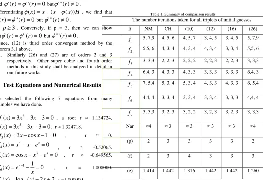
, r =1.000000.Comparisons were made relative to Newton method (NM), Chebyshev’s method (CM), and the algorithms in equations (10), (12), (14), (16), and (26). C++ implementation was done for each algorithms and the number of iterations taken to converge to a root r to six decimal places was recorded and written in the body cells of the next table-1 under each method. The stopping criteria were using the residual error
E
i=
f
(
x
i)
suchthat
f
(
x
i)
≤ε
, for chosen6
10
−=
ε
. We also checkedthis by other stopping criteria in the literature. The triplets of numbers in each cells of table-1 correspond to the
number of iterations needed for convergence for each of the three initial guesses of a root r. In the first column, ´´Functions (f) ´´ refers to the number of functional
evaluations, ´´Efficiency (e) ´´ represents the
computational efficiency index calculated by e = p1/f. The average number of iteration Nar is estimated.
Table 1. Summary of comparison results
The number iterations taken for all triplets of initial guesses
fi NM CH (10) (12) (16) (26)
1
f
5, 7,9 4, 5, 6 4, 5, 7 3, 4, 5 3, 4, 5 5, 7,92
f
5,5, 6 4, 3, 4 4, 3, 4 4, 3, 4 3, 3, 4 5,5, 63
f
3, 3,3 2, 2, 3 2, 2, 2 2, 2, 3 2, 2, 3 3, 3,34
f
6,4, 3 4, 3, 3 4, 3, 3 3, 3, 3 3, 3, 3 6,4, 35
f
7, 5,4 5, 3, 4 5, 3, 4 4, 3, 3 4, 3, 3 6, 5,46
f
4,4, 4 3, 3, 4 3, 3, 4 3, 3, 4 3, 3, 3 4,4, 47
f
3, 3,3 3, 2, 3 3, 2, 2 3, 2, 3 3, 2, 3 3, 3,3Nar ≈4 ≈ 3 ≈ 3 ≈ 3 ≈ 3 ≈4
(p) 2 3 3 3 3 2
(f) 2 3 4 3 3 3
(e) 1.414 1.442 1.316 1.442 1.442 1.260
5. Some Areas of Applications
a)
Applications in Engineering Models
Here, we shall offer some realistic applications of iterative root finding. For more examples, refer to [1, 9, 10, 12].
1. Water vapor splits into Oxygen and Hydrogen at
higher temperature as [12]
2 2 2
2
H O
2
H
+
O
www.ijiset.com r = R2/R1, with concentrations R1 = [H2O]2, R2 =
[H2] 2
[O2] and
2
1
2
t
p
f
k
f
f
=
−
+
(29)Where k = 0.04 is a given reaction equilibrium constant and p t = 3.5atm is the total pressure at some temperature T. (29) is an intricate equation to determine f not easily and hence the importance of root finding. The equation to be solved for the mole fraction of water vapor in (29) becomes
( )
0.04
7
0.
1
2
f
F
F f
f
f
=
=
−
=
−
+
-2 -1 0 1 2 3 4 5 6
-2 0 2 4 6
x=f F=1/25-f/(1-f) 71/2 (1/(2+f))1/2
F
Fig-1: Graph of F indicating a root
The Newton’s method for F is
fi+1= fi-F(fi)/F’(fi) ,i=0,1,2… (3.1)
With an initial guess of f0 = 0.1, the
approximate mole fraction is f = 0.0210 in
(0, 1).
b) The model below can be used to estimate Oxygen level c (mg/l) in a river downstream from a sewage discharge [12]:
c = 10-20(e-0.15x-e-0.5x) (30)
Where x is the distance downstream in kilometers. Then we may need the value of x for which Oxygen is minimum.
We mean the zeros of the first derivative of (30), which is
p = 3e(-3/20*x)-10*e(-1/2*x) (31)
-6 -4 -2 0 2 4 6
-200 -150 -100 -50 0
x
p=3 exp(-3/20 x)-10 exp(-1/2 x)
p
Fig 2: Root location for p
Taking an initial guess x0 = 4 and applying Newton’s method we get x = 3.4399 with minium Oxygen level c = 1.6433.
3 3.1 3.2 3.3 3.4 3.5 3.6 3.7 3.8 3.9 4 3.32
3.34 3.36 3.38 3.4 3.42 3.44
x
y=x-(3 exp(-3/20 x)-10 exp(-1/2 x))/(-9/20 exp(-3/20 x)+5 exp(-1/2 x))
y
Fig 3 Newton fixed point for p on [3, 4]
6. Conclusions
In this work, we have applied derivative estimation (a very new concept in root finding) combined with Taylor’s third order approximation to obtain new iterative methods for estimating simple roots of nonlinear equations, which is our main success. We investigated algorithms which are more efficient than some existing methods. We have observed that estimation of
f
'
''
in terms of lower derivatives could result in fast convergent or efficient methods, important in science and engineering. We also presented two examples of engineering applications. In the future, we will make further analyses of these algorithms with possible extensions and other higher order iterative algorithms for multiple roots also. We hope that this result will be more precious and activate one to perform further research in the field.Acknowledgments
www.ijiset.com
References
[1] Alfio Quarteroni, Riccardo Sacco, Fausto Saleri., Numerical mathematics (Texts in applied mathematics; 37), Springer-Verlag New York, Inc., USA, 2000
[2] Anthony Ralston, Philip Rabinowitz, A first course in numerical analysis (2nd ed.), McGraw-Hill Book Company, New York, 1978
[3] Germund Dahlquist, and Ake Bjorck, Numerical methods in scientific computing Volume I, Siam - Society for industrial and applied mathematics. Philadelphia, USA, 2008
[4] Jorgen Gerlach, Accelerated Convergence in Newton’s Method, Society for industrial and applied mathematics, (1994), Siam Review 36, 272-276.
[5] J.Stoer, R. Bulirsch, Texts in Applied mathematics 12, Introduction to Numerical Analysis (2nd ed.), springer-Verlag New York, Inc., USA, 1993.
[6] Kou Jisheng, Li Yitian, Wang Xiuhua, A uniparametric Chebyshev-type method free from second derivative, Applied Mathematics and Computational, (2006), 179, 296-30
0.
[7] Ljiljana D.Petkovic, and Miodrag S.Petkovic, on the fourth order root finding methods of Euler type, NOVI SAD J.MATH.,( 2006), 36, 157-165.
[8] M.M. Hussein, A note on one-step iteration methods for solving nonlinear equations, World Applied Sciences Journal 7 (special issue for applied math), IDOSI, Publications, (2009), 90-95.
[9] Malvin R.Spencer (PhD Dissertation, 1994), Polynomial Real Root Finding in Bernstein Form, Department of engineering, Brigham Young University.
[10] Pakdemirli, H. Boyacl and H. A. Yurtsever,. A root finding algorithm with fifth order derivatives, Mathematical and Computational Applications, (2008), Vol.13, 123-128. [11] Philipp Rostalski (PHD.Thesis, 2009), Algebraic Moments –
Real Root Finding and Related Topics, ETH Zurich (TU Hamburg-Harburg, German), Dissertation ETH Zurich No. 18371
[12] Steven C Chapra, Raymond P Canale (2007), Numerical methods for engineers (5thed.), Tata McGraw-Hill, New york.
[13] Shengfeng Li and Rujing Wang, Two fourth order iterative methods based on Continued Fraction for root finding problems, World Academy of Science, Engineering and Technology 60, 2011
[14] YI JIN AND BAHMAN KALANTARI (communicated by Peter A. Clarkson), A combinatorial construction of high order algorithms for finding polynomial roots of known multiplicity, American Mathematical Society, (2010), 138, 1897-1906.
Author’s Biography
Name: Tekle Gemechu (PHD) BSC in applied mathematics (1997) MSC in numerical analysis (2004)
PHD in applied maths (computational maths) (2014) Title (Rank): Assistant professor