Curves
Koray Karabina
Florida Atlantic University, Boca Raton, FL, 33433, USA, [email protected]
Abstract. We analyze the point decomposition problem (PDP) in binary elliptic curves. It is known that PDP in an elliptic curve group can be reduced to solving a particular system of multivariate non-linear system of equations derived from the so called Semaev summation polynomials. We modify the underlying system of equations by introducing some auxiliary variables. We argue that the trade-off between lowering the degree of Semaev polynomials and increasing the number of variables provides a significant speed-up.
Keywords: Semaev polynomials, elliptic curves, point decomposition problem, discrete logarithm problem
1
Introduction
Thepoint decomposition problem (PDP) in an additive abelian groupGwith respect to afactor base B ⊂Gis the following: Given a point1 R∈G, findPi∈ Bsuch that
R=
m
X
i=1
Pi
for some positive integerm; or conclude thatRcannot be decomposed as a sum of points in B. Thediscrete logarithm problem (DLP) in Gwith respect to a base P ∈Gis the following: GivenP andQ=aP ∈Gfor some secret integera, computea. DLP can be solved using the index calculus algorithm in two main steps. In therelation collection step, fix a factor base B, and find a set of points Ri = aiP+biQ for some randomly
chosen integersai, bi, such thatRi can be decomposed with respect toB, i.e.,
Ri=
X
j
Pij, Pij ∈ B.
Here, we may assume for convenience thatPijare not necessarily distinct. Note that each
decomposition induces a modular linear dependence on the discrete logarithms ofQ∈G and Pij ∈ B with respect to the base P. After collecting sufficiently many relations2,
linear algebra step solves for the discrete logarithm of Q ∈ G, as well as the discrete logarithms of the factor base elements. Clearly, the success probability and the running time of the index calculus algorithm heavily depend on the decomposition probability of a random element in G, the cost of the decomposition step, and the size of the factor
1 We prefer to usepointrather thanelementbecause elliptic curve group elements are commonly
called points.
base. In particular, the overall cost of the relation collection and the linear algebra steps must be optimized with a non-trivial success probability.
In 2004, Semaev [11] showed that solving PDP in an elliptic curve group is equivalent to solving a particular system of multivariate non-linear system of equations derived from the so calledSemaev summation polynomials. Semaev’s work triggered the possibility of the existence of an index calculus type algorithm which is more efficient than the Pollard’s rho algorithm to solve the discrete logarithm problem in elliptic curves defined overFqn, which we denote ECDLP(q, n). Note that Pollard’s rho algorithm is a general purpose algorithm that solves DLP in a groupG, and runs in timeO(p|G|). Gaudry [7] showed that, for a fixed n, Semaev summation polynomials can be effectively used to solve ECDLP(q, n) in heuristic timeO(q2−2
n), where the constant inO(·) is exponential inn. For example, Gaudry’s algorithm and Pollard’s rho algorithm solve ECDLP(q,3) in time
O(q1.33) and O(q1.5), respectively. Due to the exponential inn constant in the running time of Gaudry’s algorithm, his attack is expected to be more effective than Pollard’s rho algorithm if n ≥ 3 is relatively small and q is large. Diem [2] rigorously showed that ECDLP(q, n) can be solved in an expected subexponential time whena(logq)α≤
n ≤b(logq)β for some a, b, α, β > 0. On the other hand, Diem’s method has expected exponential running timeO(en(logn)1/2
) for solving ECDLP(2, n). As a result, the index calculus type algorithms presented in [7, 2] do not yield ECDLP solvers which are more effective than Pollard’s rho method when q= 2 andnis prime. The ideas for choosing an appropriate factor base in [2] have been adapted in [5, 10], and the complexity of the relation collection step have been analyzed. In both papers [5] and [10], a positive integer
m, which we call thedecomposition constant, is fixed to represent the number of points in the decomposition of a random point in the relation collection step. The factor base consists of elliptic curve points whosex-coordinates belong to ann0-dimensional subspace
V ⊂F2n overF2, wheren0 is chosen such thatmn0 ≈n. We refer to PDP in this setting by PDP(n, m, n0) throughout the rest of this paper.
Faug`ere et al. [5] showed, under a certain assumption, that ECDLP(2, n) can be solved in timeO(2ωn/2), where 2.376≤ω≤3 is the linear algebra constant. The running time analysis in [5] considers the linearization technique to solve the multivariate nonlinear system of equations which are derived from the (m+ 1)’st Semaev polynomial Sm+1 during the relation collection step to solve PDP(n, m, n0). Faug`ere et al. further argue that, Groebner basis techniques may improve the running time by a factor m in the exponent, where m is the decomposition constant. This last claim has been confirmed in the experiments in [5] for elliptic curves defined over F2n with n ∈ {41,67,97,131} and m = 2. Petit and Quisquater’s heuristic analysis in [10] claims that ECDLP(2, n) can asymptotically be solved in time O(2cn2/3logn) for some constant 0 < c < 2. The
subexponential running time in [10] is based on a rather strong assumption on the be-havior of the systems of equations that arise from Semaev polynomials. In particular, it is assumed in [10] that the degree of regularity Dreg and the first fall degreeDFirstFall of
the underlying polynomial systems to solve PDP(n, m, n0) are approximately equal. The analysis in [10] also assumes thatn0 =nα and m=n1−α for some positive constantα. Experiments with a very limited set of parameters (n, m, n0),n ∈ {11,17}, m∈ {2,3},
n0=dn/mewere conducted in [10] in the favor of their assumption.
[13] were able to extend their experimental data for the parameters (n, m, n0, ∆),n≤48,
m= 2, and where∆=n−mn0 is chosen appropriately to possibly improve the running time of ECDLP(2, n). In another recent paper [8], Huang et al. exploit the symmetry in Semaev polynomials, and improve on the running time and memory requirements of the PDP(n, m, n0) solver in [5]. The efficiency of the method in [8] is tested for parameters (n, m, n0) such thatn≤53,m= 3, n0= 3,4,5,6.
Petit and Quisquater’s heuristic analysis [10] claims that index calculus methods for solving ECDLP(2, n) is more effective than the Pollard’s rho method forn >2000,m≥4 andmn0≈n. However, all the experiments reported so far on solving PDP(n, m, n0) for the set of parameters (n, m, n0, ∆) with ∆ = n−mn0 ≤ 1 and m = 3 are limited to
n≤19; see [13, 8]. Similarly, all the experiments for the set of parameters (n, m, n0, ∆) withm= 3 are limited ton0≤6, which forces∆≥2 forn≥20. In general, it is desired to haven0 increasing as a function ofn, rather than having some upper bound onn0, so thatn≈mn0 as assumed in the running time analysis of ECDLP(2, n) solvers in [5, 10]. Therefore, it remains a challenge to run experiments on an extensive set of parameters (n, m, n0) with larger primen values,m≥4, andmn0≈n. For example, it is stated in [8, Section 4.1] that
On the other hand, the method appears unpractical form= 4 even for very small values ofnbecause of the exponential increase withmof the degrees in Semaev’s polynomials.
In a more recent paper [6], Galbraith and Gebregiyorgis introduce a new choice of variables and a new choice of factor base, and they are able to solve PDP with various
n≥17,m= 4,n0 = 3,4 using Groebner basis algorithms; and also with variousn≥17,
m= 4, n0≤7 using SAT solvers.
In this paper, we modify the system of equations, that are derived from Semaev poly-nomials, by introducing some auxiliary variables. We show that PDP(n, m, n0) can be solved by finding a solution to a system of equations derived from several third Se-maev polynomials S3 each of which has at most three variables. For a comparison, PDP(n, m, n0) in E(F2n) with decomposition constant m = 5 would be traditionally attacked via considering the Semaev polynomial S6 with 5 variables, which is likely to have a root inV5, whereV ⊂
F2n is a subspace of dimensionn0 =bn/5c. On the other hand, when m = 5, our polynomial system consists of third Semaev polynomials S3,i
(i= 1,2,3,4), and a total of 8 variables which is likely to have a root inV5×F32n, where
V ⊂F2nis a subspace of dimensionbn/5c. As a result, our technique overcomes the diffi-culty of dealing with the (m+1)’st Semaev polynomialSm+1when solving PDP(n, m, n0) withm≥4. We should emphasize that choosingm≥4 is desirable for an index calculus based ECDLP(2, n) solver to be more effective than a generic DLP solver such as Pol-lard’s rho algorithm. Our method introduces an overhead of introducing some auxiliary variables. However, we argue that the trade-off between lowering the degree of Semaev polynomials and increasing the number of variables provides a significant speed-up. In particular, we present some experimental results on solving PDP(n, m, n0) for the follow-ing parameters:
– n ≤19, m = 4,5, and n0 =bn/mc. We are not aware of any previous experimental data forn >15 andm= 5.
– n≤26,m= 3,n0 =bn/mc. We are not aware of any previous experimental data for
n >21,m= 3, and∆=n−mn0≤2.
can be improved significantly if the Groebner basis computations are first performed on a subset of polynomials and if the ReductionHeuristic parameter in Magma is set to be a small number; see Section 5 for more detail. We would like to emphasize that these techniques are aplied for the first time in this paper to solve the point decomposition problem. As a result, we gain significant improvement over the recently published ex-perimental results [12]. For a comparison, we are able to solve PDP(15,5,3) instances in about 7 seconds (with 256 MB memory). Note that, PDP(15,5,3) is solved in about 175 seconds (with 2635 MB memory) in [12]. In general, our experimental findings with
m= 3,4,5 extend and improve on the recently reported results in [13, 8, 12].
The rest of this paper is organized as follows. In Section 2, we recall Semaev poly-nomials and their application to ECDLP(2, n). In Section 3, we describe and analyze a new method to solve PDP(n, m, n0) inE(F2n). In Section 4, we present our experimental results. In Section 5, we extend our results from Section 3.
2
Semaev Polynomials and ECDLP
Let F2n =F2[σ]/hf(σ)i be a finite field with 2n elements, where f(σ) is a monic irre-ducible polynomial of degreenover the fieldF2={0,1}. letE be a non-singular elliptic curve defined by the short Weierstrass equation
E/F2n: y2+xy=x3+ax2+b, a, b∈F2n.
We denote the identity element ofEby∞. Thei’th Semaev polynomial associated with
E is defined as follows:
Si(x1, x2, . . . , xi) =
(
(x1x2+x1x3+x2x3)2+x1x2x3+b ifi= 3
ResX(Si−j(x1, . . . , xi−j−1, X), Sj+2(xi−j, . . . , xi, X)) ifi≥4,
(1)
where 1≤j≤i−3. Forn0 ≤n, let
V ={a0+a1σ+· · ·+an0−1σn 0−1
: ai∈F2} ⊂F2n
and define the factor base
B={P= (x, y)∈E: x∈V}.
Recall that in PDP(n, m, n0), we are looking forPi= (xi, yi)∈ Bsuch that
P1+· · ·Pm=R, (2)
for some given point R= (xR, yR)∈E. We refer to (2) as an m-decomposition ofR in B. We expect that, on average, a random pointR∈Ehas anm-decomposition inBwith probability 2mn0/2nm! simply because|B| ≈2n0 and permutingP
i does not change the
sumPP
i (see [7]). As described in Section 1, the DLP inEcan be solved via an
index-calculus based approach by computing about|B|explicitm-decompositions and solving a sparse linear system of about|B|equations. Therefore, the cost of solving ECDLP(2, n) may be estimated as
2n02
nm!
2mn0Cn,m,n0+ 2
whereCn,m,n0 is the cost of solving PDP(n, m, n0), andω0= 2 is the sparse linear algebra
constant. Semaev [11] showed that a decomposition of the form (2) exists if and only if the x-coordinates of Pi and R are zeros of the (m+ 1)’st Semaev polynomial, that is,
Sm+1(x1, . . . , xm, xR) = 0. In the rest of this paper, we focus on solving PDP(n, m, n0)
(and estimatingCn,m,n0) via modifying the equation induced bySm+1.
3
A new approach to solve the point decomposition problem
Let E/F2n, V, and B be as defined in Section 2. Recall that an m-decomposition of a point
R=P1+· · ·Pm,
whereR= (xR, yR)∈E,Pi= (xi, yi)∈ B, can be computed (if exists) by identifying a
tuple (x1, . . . , xm)∈Vm that satisfies
Sm+1(x1, . . . , xm, xR) = 0 (4)
Note thatxibelong to ann0-dimensional subspace ofF2n. Therefore, (4) defines a system
Sys1 of a single equation over F2n in m variables. In [5, 10], the Weil descent technique is applied, and a second system Sys2 of n equations over F2 in mn0 boolean variables is derived from Sys1. The cost Cn,m,n0 of solving PDP(n, m, n0) in [5, 10] is estimated
through the analysis of solving Sys2 using linearization and Groebner basis techniques. Next, we describe a new approach to derive another system Sys3 of boolean equations such that a solution ofSys3 yields anm-decomposition of a pointR.
Notation. Throughout the rest of this paper, we distinguish between two classes Semaev polynomials. The first class of Semaev polynomials is denoted bySm,1(x1, . . . , xm), which
represents the m’th Semaev polynomial with m variables. The second class of Semaev polynomials is denoted by Sm,2(x1, . . . , xm−1, xR), which represents the m’th Semaev
polynomial withm−1 variables (i.e., the last variablexmis evaluated at a numberxR).
3.1 The case:m = 3
LetR= (xR, yR)∈E. Notice that there existPi∈ Bsuch that
P1+P2+P3−R=∞
if and only if there existPi ∈ BandP12∈Esuch that
(
P1+P2−P12=∞
P3+P12−R=∞
(5)
Therefore, a 3-decomposition ofR=P1+P2+P3 may be found as follows:
1. Define the following system of equations derived from Semaev polynomials
(
S3,1(x1, x2, x12) = 0
S3,2(x3, x12, xR) = 0.
(6)
2. Introduce boolean variables xi,j such that
xi= n0−1
X
j=0
xi,jσj,
fori= 1,2,3, and
x12=
n
X
j=0
x12,jσj.
Apply the Weil descent technique to (6) and define an equivalent system of 2n equa-tions overF2 with 3n0+nboolean variables
{xi,j: i= 1,2,3, j= 0, . . . n0−1} ∪ {x12,j : j= 0, . . . n−1}.
Solve this new system of boolean equations and recoverx1, x2, x3∈F2n from xi,j∈ F2.
Note that the proposed method solves a system of 2nequations overF2 with 3n0+n boolean variables rather than solving a system of nequations overF2 with 3n0 boolean variables.
3.2 The case:m = 4
LetR= (xR, yR)∈E. Notice that there existPi∈ Bsuch that
P1+P2+P3+P4−R=∞
if and only if there existPi ∈ BandP12∈Esuch that
(
P1+P2−P12=∞
P3+P4+P12−R=∞
(7)
Therefore, a 4-decomposition ofR=P1+P2+P3+P4 may be found as follows:
1. Define the following system of equations derived from Semaev polynomials
(
S3,1(x1, x2, x12) = 0
S4,2(x3, x4, x12, xR) = 0
(8)
Note that this system is defined overF2n and has 5 variablesx1, x2, x3, x4, x12. 2. Introduce boolean variables xi,j such that
xi= n0−1
X
j=0
xi,jσj,
fori= 1,2,3,4, and
x12=
n
X
j=0
xi,jσj.
Apply the Weil descent technique to (8) and define an equivalent system of 2n equa-tions overF2 with 4n0+nboolean variables
{xi,j: i= 1,2,3,4j= 0, . . . n0−1} ∪ {x12,j : j= 0, . . . n−1}.
Solve this new system of boolean equations and recover x1, x2, x3, x4 ∈ F2n from
Note that the proposed method solves a system of 2nequations overF2 with 4n0+n boolean variables rather than solving a system of nequations overF2 with 4n0 boolean variables.
3.3 The case:m = 5
LetR= (xR, yR)∈E. Notice that there existPi∈ Bsuch that
P1+P2+P3+P4+P5−R=∞
if and only if there existPi ∈ BandP123∈E such that
(
P1+P2+P3−P123=∞
P4+P5+P123−R=∞
(9)
Therefore, a 5-decomposition ofR=P1+P2+P3+P4+P5may be found as follows:
1. Define the following system of equations derived from Semaev polynomials
(
S4,1(x1, x2, x3, x123) = 0
S4,2(x4, x5, x123, xR) = 0
(10)
Note that this system is defined overF2n and has 6 variablesx1, x2, x3, x4, x5, x123. 2. Introduce boolean variables xi,j such that
xi= n0−1
X
j=0
xi,jσj,
fori= 1,2,3,4,5, and
x123=
n
X
j=0
x123,jσj.
Apply the Weil descent technique to (10) and define an equivalent system of 2n
equations overF2 with 5n0+nboolean variables
{xi,j: i= 1,2,3,4,5j= 0, . . . n0−1} ∪ {x123,j : j = 0, . . . n−1}.
Solve this new system of boolean equations and recoverx1, x2, x3, x4, x5∈F2n from
xi,j∈F2.
Note that the proposed method solves a system of 2nequations overF2 with 5n0+n boolean variables rather than solving a system of nequations overF2 with 5n0 boolean variables.
3.4 Analysis of the new polynomial systems
One of the methods to solve a multivariate non-linear system of equations is to com-pute the Groebner basis of the underlying ideal. Groebner basis computations can be performed using Faug`ere’s algorithms [3, 4], which reduce the problem to Gaussian elim-ination of Macaulay-type matrices Md of degree d. The Macaulay matrix Md encodes
Therefore, the cost of solving a system of equations is determined by the maximal degree
D (also known as the degree of regularity of the system) reached during the compu-tation. If N is the number of variables in the system, then the cost is estimated as
O N+DD−1ω
, where N+DD−1
is the maximum number of columns inMDandωis the
linear algebra constant. In general, it is hard to estimateD. In the recent paper [10], it is conjectured that the degree of regularity Dreg of systems arising from PDP(n, m, n0)
satisfies Dreg =DFirstFall+o(1), whereDFirstFall is the first fall degree of the system and
defined as follows.
Definition 1. [10] LetR be a polynomial ring over a fieldK. LetF:={f1, . . . , f`} ⊂R be a set of polynomials of degrees at mostDFirstFall. The first fall degree ofFis the smallest
degree DFirstFall such that there exist polynomials gi∈R with maxi(deg(fi) + deg(gi)) =
DFirstFall, satisfyingdeg(P `
i=1gifi)< DFirstFallbut P `
i=1gifi 6= 0.
Experimental studies in recent papers [10, 13] give supporting evidence that Dreg ≈
DFirstFall. However, experimental data is yet very limited (see Section 1) to verify this
conjecture. In this section, we compute the first fall degree of the systems proposed in Section 3.1, Section 3.2, and Section 3.3. Our experimental results in Section 4 support thatDreg≈DFirstFall.
DFirstFall of the system whenm = 3 In this case, one needs to solve the system of 2n equations overF2with 3n0+nboolean variables. The system of equations is derived by applying Weil descent to (6) that consists of two Semaev polynomialsS3,1 andS3,2. The monomial set ofS3,1(x1, x2, x12) is
{1, x21x22, x21x212, x22x212, x1x2x12}.
Therefore, the Weil descent ofS3,1(x1, x2, x12) yields a 2n0+nvariable polynomial set
{fi} over F2 such that maxi(deg(fi)) = 3. On the other hand, the monomial set of
x1·S3,1(x1, x2, x12) is
{x1, x31x 2 2, x
3 1x
2 12, x
2 2x
2 12, x
2 1x2x12}.
Therefore, the Weil descent of x1 ·S3,1(x1, x2, x12) yields a polynomial set {Fi} over F2 such that maxi(deg(Fi)) = 3. It follows from the definition thatDFirstFall(S3,1) ≤ 4 because the maximum degree of polynomials obtained from the Weil descent of x1 is 1. Similarly, the monomial set ofS3,2(x3, x12, xR) is
{1, x23x212, x32, x212, x3x12}.
Therefore, the Weil descent of S3,2(x3, x12, xR) yields a n0+n variable polynomial set {fi} over F2 such that maxi(deg(fi)) = 2. On the other hand, the monomial set of
x3
3·S3,2(x3, x21, xR) is
{x33, x53x212, x53, x33x212, x43x12}.
Therefore, the Weil descent of x3
3·S3,2(x3, x12, xR) yields a polynomial set {Fi} over
F2 such that maxi(deg(Fi)) = 3. It follows from the definition thatDFirstFall(S3,2) ≤ 4 because the maximum degree of polynomials obtained from the Weil descent of x33 is 2. We conclude thatDFirstFall≤4.
and S4,2. From our above discussion, DFirstFall(S3,1)≤4. Now, analyzing the monomial set of S4,2(x3, x4, x123, xR), we can see that the Weil descent of S4,2(x3, x4, x123, xR)
yields a 2n0+n variable polynomial set{fi} over
F2 such that maxi(deg(fi)) = 6 (this
follows from the Weil descent of the monomial (x3x4x123)3). On the other hand, an-alyzing the monomial set of x3·S4,2(x3, x4, x123, xR), we see that the Weil descent of
x3·S4,2(x3, x4, x123, xR) yields a polynomial set{Fi}overF2such that maxi(deg(Fi)) = 6.
It follows from the definition that DFirstFall(S4,2) ≤ 7 because the maximum degree of polynomials obtained from the Weil descent ofx3 is 1. We conclude thatDFirstFall≤7.
DFirstFall of the system when m= 5 In this case, one needs to solve the system of 2n equations over F2 with 5n0 +n boolean variables. The system of equations is de-rived by applying Weil descent to (10) that consists of two Semaev polynomialsS4,1and
S4,2. From our above discussion, DFirstFall(S4,2) ≤ 7. Now, analyzing the monomial set ofS4,1(x1, x2, x3, x123), we can see that the Weil descent ofS4,1(x1, x2, x3, x123) yields a 3n0+nvariable polynomial set{fi}overF2such that maxi(deg(fi)) = 8 (this follows from
the Weil descent of the monomial (x1x2x3x123)3). On the other hand, analyzing the mono-mial set ofx3·S4,1(x1, x2, x3, x123), we see that the Weil descent ofx3·S4,1(x1, x2, x3, x123) yields a polynomial set {Fi} over F2 such that maxi(deg(Fi)) = 8. It follows from the
definition thatDFirstFall(S4,1)≤9 because the maximum degree of polynomials obtained from the Weil descent ofx3 is 1. We conclude thatDFirstFall≤9.
4
Experimental results
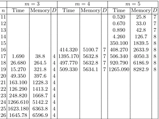
We implemented the methods proposed in Section 3 on a desktop computer (Intel(R) Xeon(R) CPU E31240 3.30GHz) using Groebner basis algorithms in Magma [1]. For each parameter set (n, m, n0), we solved 5 random instances of PDP over a randomly chosen elliptic curveE/F2n. In Table 1, we report on our experimental results for solving PDP(n, m, n0=bn/mc) withm= 3,4,5. In particular, for each of these 5 computations, we report on the maximum CPU time (seconds) and memory (MB) required for solving PDP. We also report on the maximum of the maximum step degreesD in the Groebner basis computations. Recall that in Section 3, we estimated DFirstFall ≤ 4 when m = 3;
DFirstFall≤7 whenm= 4; andDFirstFall≤9 whenm= 5. In our experiments, we observe
thatDreg= 4 whenm= 3;Dreg = 7 whenm= 4; and Dreg≤8 when m= 5.
Letm= 5 andn0=bn/mc. Based on our experimental data, it is tempting to assume that the underlying system of polynomial equations hasDreg≤9. Moreover, the system
hasN = 5n0+n≈2nboolean variables. Therefore, whenm= 5, we may estimate the cost of solving ECDLP(2, n) (see (3)) as
2n02
nm!
2mn0
N+D
reg−1
Dreg
w + 2w0n0
≈2n/5m!(2n)9w+ 2w0n/5
≈2342n/5n27+ 22n/5,
Table 1.Experimental results on solving PDP(n, m, n0 =bn/mc). Time in seconds; Memory in MB;Dis the maximum step degree.
m= 3 m= 4 m= 5
n Time MemoryD Time MemoryD Time MemoryD
11 0.520 25.8 7
12 0.670 33.0 7
13 0.890 42.8 7
14 4.260 126.7 8
15 350.100 1839.5 8
16 414.320 5100.7 7 408.270 2633.9 8 17 1.690 38.8 4 1395.170 5632.8 7 506.340 4050.3 8 18 26.680 264.5 4 497.770 5632.8 7 920.790 6186.9 8 19 15.270 321.8 4 509.330 5634.1 7 1265.090 8282.9 8 20 49.350 397.6 4
21 163.100 1228.3 4 22 126.290 1413.2 4 23 248.820 1668.7 4 24 1266.610 5142.2 4 25 1623.180 6363.8 4 26 1645.78 6596.9 4
5
Extensions and Optimization
In Section 3, we introduced a single auxiliary variable to lower the degree of Semaev polynomials. The degree of polynomials can further be lowered by introducing more auxiliary variables. As an example, we consider the casem= 5. LetR = (xR, yR)∈E,
as before. Notice that there existPi∈ Bsuch that
P1+P2+P3+P4+P5−R=∞
if and only if there existPi ∈ BandP12, P34, P50∈E such that
P1+P2−P12=∞
P3+P4−P34=∞
P5−P50−R=∞
P12+P34+P50=∞
(11)
Therefore, a 5-decomposition ofR=P1+P2+P3+P4+P5may be found as follows:
1. Define the following system of equations derived from Semaev polynomials
S3,1(x1, x2, x12) = 0
S3,1(x3, x4, x34) = 0
S3,2(x5, x50, xR) = 0
S3,1(x12, x34, x50) = 0
(12)
Note that this system is defined overF2nand has 8 variablesx1, x2, x3, x4, x5, x12, x34, x50. 2. Introduce boolean variables xi,j such that
xi= n0−1
X
j=0
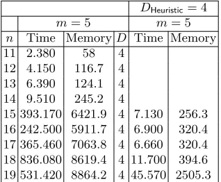
Table 2.Experimental results on solving PDP(n, m, n0 =bn/mc). Time in seconds; Memory in MB;Dis the maximum step degree;DHeuristic is set to be 4 in Groebner basis computations.
DHeuristic= 4
m= 5 m= 5
n Time MemoryD Time Memory 11 2.380 58 4
12 4.150 116.7 4 13 6.390 124.1 4 14 9.510 245.2 4
15 393.170 6421.9 4 7.130 256.3 16 242.500 5911.7 4 6.900 320.4 17 365.460 7063.8 4 6.660 320.4 18 836.080 8619.4 4 11.700 394.6 19 531.420 8864.2 4 45.570 2505.3
fori= 1,2,3,4,5, and
xi,j= n
X
k=0
xi,jσj,
fori= 12,34,50. Apply the Weil descent technique to (12) and define an equivalent system of 4nequations overF2 with 5n0+ 3nboolean variables
{xi,j: i= 1,2,3,4,5 j= 0, . . . n0−1} ∪ {xi,j: i= 12,34,50, j= 0, . . . n−1}.
Solve this new system of boolean equations and recoverx1, x2, x3, x4, x5∈F2n from
xi,j∈F2.
Note that the proposed method solves a system of 4nequations overF2with 5n0+ 3n boolean variables rather than solving a system of nequations overF2 with 5n0 boolean variables. Similar to the analysis in Section 3, we can show thatDFirstFall≤4.
In Table 2, we report on our experimental results for solving PDP(n, m, n0 =bn/mc) withm= 5 deploying only the third Semaev polynomials; see (12). The time and memory results in the second and third column of Table 2 are obtained using the Groebner basis implementation of Magma with thegrevlexordering of monomials. We observe that the maximum step degree isDreg= 4 for 11≤n≤19. The time and memory results in the
last two columns of Table 2 are obtained using the Groebner basis implementation of Magma with thegrevlexordering of monomials in a boolean ring. We also introduced two modifications in the computations: We set theReductionHeuristicparameter in Magma to 4; and we first computed Groebner bases of partial systems described by single equations in (12), and merged them later. These two techniques yield non-trivial optimization both in time and memory. For a comparison, whenn= 15 andm= 3, (Time, Memory) values decrease from (393.170,6421.9) to (7.130,256.3) when this modification is deployed in the computation; see Table 2. For the same parameters (n = 15 and m = 3), (Time, Memory) values are reported as (174.47,2635.4) in [12].
Based on our experimental data, it is tempting to assume that the underlying system of polynomial equations hasDreg ≤4 for alln. Moreover, the system hasN = 5n0+ 3n≈
ECDLP(2, n) (see (3)) as
2n02
nm!
2mn0
N+D
reg−1
Dreg
w + 2w0n0
≈2n/5m!(4n)4w+ 2w0n/5
≈2312n/5n12+ 22n/5,
where we assumew= 3 andw0 = 2. This running time outperforms square-root methods whenn >457. For example, whenn≈550, the cost of solving ECDLP(2, n) is estimated to be 2250which is significantly smaller than the cost 2275of square-root time algorithms.
Acknowledgment
I would like to acknowledge two recent papers [12, 9]. Semaev [12] claims a new com-plexity bound 2c(√nlnn) for solving ECDLP(2, n) under the assumption that the degree
of regularity in Groebner computations of particular polynomial systems is Dreg ≤ 4.
Semaev also shows that ECDLP(2, n) can be solved in time 2o(c√nlnn) under a weaker assumption that Dreg =o(
p
n/lnn) The techniques used in [12] and in this paper are similar. In [9], Kosters and Yeo provide experimental evidence that the degree of regular-ity of the underlying polynomial systems is likely to increase as a function ofn, whence the conjectureDreg≈DFirstFall may be false.
I would like to thank Michiel Kosters and Igor Semaev for their comments on the first version of this paper.
References
1. W. Bosma, J. Cannon, and C. Playoust,The Magma algebra system I: The user language, Journal of Symbolic Computation24(1997), 235–265.
2. C. Diem,On the discrete logarithm problem in elliptic curves II, Algebra and Number Theory
7(2013), 1281–1323.
3. J.-C. Faug`ere, A New efficient algorithm for computing Groebner bases (F4), Journal of Pure and Applied Algebra139(1999), 61–68.
4. ,A New efficient algorithm for computing Groebner bases without reduction to zero (F5), International Symposium on Symbolic and Algebraic Computation (2002), 75–83. 5. J.-C. Faug`ere, L. Perret, C. Petit, and G. Renault,Improving the complexity of index calculus
algorithms in elliptic curves over binary fields, Advances in Cryptology – EUROCRYPT 2012, Lecture Notes in Computer Science7237(2012), 27–44.
6. S. Galbraith and S. Gebregiyorgis,Summation polynomial algorithms for elliptic curves in characteristic two, Advances in Cryptology – INDOCRYPT 2014, Lecture Notes In Com-puter Science8885(2014), 409–427.
7. P. Gaudry, Index calculus for abelian varieties of small dimension and the elliptic curve discrete logarithm problem, Journal of Symbolic Computation44(2009), 1690–1702. 8. Y.-J. Huang, C. Petit, N. Shinohara, and T. Takagi,Improvement of Faug`ere et al.’s method
to solve ECDLP, Advances in Information and Computer Security, Lecture Notes in Com-puter Science8231(2013), 115–132.
9. M. Kosters and S. Yeo,Notes on summation polynomials, (2015), arXiv:1503.08001. 10. C. Petit and J.-J. Quisquater,On polynomial systems arising from a Weil descent, Advances
11. I. Semaev, Summation polynomials and the discrete logarithm problem on elliptic curves, Cryptology ePrint Archive: Report 2004/031, 2004.
12. ,New algorithm for the discrete logarithm problem on elliptic curves, (2015), Cryp-tology ePrint Archive: Report 2015/310.