Differentiation operation in the wave equation for the pseudospectral method
with a staggered mesh
Zhixin Zhao1, Jiren Xu1, and Shigeki Horiuchi2
1Institute of Geology, Chinese Academy of Geological Science, Beijing 100037, China
2National Research Institute for Earth Science and Disaster Prevention (NIED), Science and Technology Agency, 3-1 Tennodai, Tsukuba-shi, Ibaraki-ken 305-0006, Japan
(Received March 31, 2000; Revised March 1, 2001; Accepted March 2, 2001)
In the present analysis we introduced a calculation strategy of the staggered grid differentiation by using the real value FFT and real inverted FFT for the pseudospectral method and applied the technique to seismic wave simulation. The calculation method introduced here is one third faster on average than the traditional differentiation method by using the complex FFT. The introduced differentiation strategy is very efficient in economy. For example we apply the staggered grid differentiation by real valued FFT to the simulation of seismic wave propagation in inhomogeneous medium. The results show the validity of the present method.
1.
Introduction
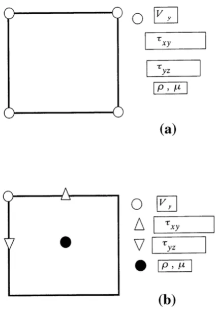
The pseudospectral (PS) method was employed in the cal-culations for fluid dynamics by Orszag (1972). The method has also been employed widely in the simulations of acous-tic wave and elasacous-tic wave equations because of its high ac-curacy and efficiency in use of the computer memory com-pared with the other discrete numerical method (Kosloff and Baysal, 1982; Fornberg, 1987; Reshefet al., 1988). The time differentiation in the PS method is generally performed by using a second order centered differential operator same as that in the finite difference method (FD) in the computation of synthetic seismograms. The spatial partial differentiation scheme of PS method, however, is different from that of the finite difference method. The spatial differentiation is per-formed through the operators of a pair of discrete Fourier transform and discrete inverse Fourier transform in the PS method (Ozdenvar and McMechan, 1996; Furumuraet al., 1998; Zhao and Kubota, 1999). The Hartley transform is also applied for the spatial differentiation in seismic simulation to improve the speed of differentiation operation (Saatcilar and Ergintav, 1991; Zhou, 1992). The Fourier transform of a discrete real sequence for a seismic wave simulation can be performed by a complex FFT in the PS method. It also can more efficiently be performed by a real FFT in the tradi-tional PS calculation in which the interested study domain is meshed with a centered mesh scheme (Fig. 1(a)). We call the meshed scheme as conventional meshed scheme in order to distinguish it from the staggered grid scheme (Fig. 1(b)). In conventional meshed scheme the relative physical variables are generally all sampled at the identical discretized nodes. The spatial derivatives of the variables are evaluated at the same nodes.
Copy right cThe Society of Geomagnetism and Earth, Planetary and Space Sciences (SGEPSS); The Seismological Society of Japan; The Volcanological Society of Japan; The Geodetic Society of Japan; The Japanese Society for Planetary Sciences.
A different discrete grid scheme, the staggered grid strat-egy, has been presented in the spatial numerical differen-tiation operator because of the more physical and accurate nature. Virieux (1984 and 1986) applied the staggered grid scheme in the FD method. Chen (1996) and Witte (1989) in-troduced the staggered grid scheme in the PS method to avoid the loss of the Nyquist component. Figure 1(b) shows the sampled parameters for a 2-D S H wave propagation of the elastic dynamic problem. In the staggered grid case, some components of variables are sampled and evaluated at the discretized nodes. The other components (even for the com-ponents of identical variable), however, are sampled half-way between the discreteized nodes (taken 1/2 simple shift in the Cartesian coordinates axes). The spatial differentiation is evaluated at the midway between grid points for a problem of the staggered grid scheme. For example in Fig. 1(b), the velocity of mediaVy is defined at the node of grid(n,m), the stressesτx y andτyz are defined at the halfway between the nodes in horizontal and vertical directions, respectively. The Lame constantμ and the densityρ can be defined at the center of grid. The numerical scheme of 2-D S H wave equation can be expressed as follows,
ρn,mv˙yn,m=∂τ˙x yn+1/2,m/∂x+∂τ˙yzn,m+1/2/∂z+ fy. (1)
Such differentiation operators of the first and second terms in the right hand side of (1) should be evaluated at the mid-way between the nodes, (n +1/2)x and(m+1/2)z, respectively.
The differential operator can be performed by the com-plex FFT. We, however, prefer to present a strategy for the staggered grid differential operator by using the real valued FFT and inverse FFT in the following section. The method is called as “RFFT staggered differentiation” for short.
Fig. 1. The sampled parameters for a 2-DS Hproblem. a) The conventional grid scheme; b) The staggered grid scheme. Vy: velocity;τx yandτyz: stresses;μ: Lame constant;ρ: density.
2.
Expansion of Fourier Series
After the analysis by Furumuraet al.(1998) afinite Fourier series expansion of a real sequence f(nx) (n=0,1, . . . ,
3.
Complex Differentiation for the Staggered Grid
Case
As respect to complex differential operator in the conven-tional mesh scheme, coefficients of the Fourier transform (FT) of real series (e.g. V orτ in (1)) are conjugate sym-metric about the Nyquist term and the imaginary parts of Nyquist terms are zero. In order to obtain a real differential result for original real series, the FT coefficients multiplied by wavenumberlkwith imaginary numberialso should be a conjugate symmetric one and the imaginary part of Nyquist term should be zero (real coefficient already becomes zero). So the imaginary part of Nyquist term forced to be zero in the inverse Fourier transform. The Nyquist information is lost.
As the spatial differentiation of variable V andτ in the wave problem in (1) are operated in a staggered meshed scheme in the PS method, derivatives in (1) are evaluated at the position of midway between the discretized grids(n+
1/2)x, shifting a 1/2 sample. The expression of complex differentiation is as follows (Witte, 1989):
d+f(x)/d x =d f((n+1/2)x)/d x
It can be seen that spectral differential operator in the con-ventional mesh scheme,ilk, has been replaced by the stag-gered spectral differential operator in (6),ilkexp(iπl/N). The Nyquist wavenumber (asl = N/2) in (6) is no longer equal to zero, being (−π/x), a purely real. So the numer-ically computed derivative is also purely real. The Nyquist information about the original function is retained through-out the process. Because Nyquist information is preserved and used, the staggered differential operators are more local. The nonzero Nyquist term makes the differentiation operator (6) more stable in the PS method. It is different from that in the conventional mesh scheme. The differentiation can also be performed by using complex FFT through transforming the real sequence into complex one in which the imaginary components arefilled up with zero values, or separating the real sequence in to real and imaginary parts of a complex one. Then it is transformed back to the physic domain by using the complex inverse FFT.
4.
Real Fourier Differentiation Method for the
Staggered Grid Case
d+f(x)/d x
After the proper trigonometric operators, Eq. (7) becomes as follows,
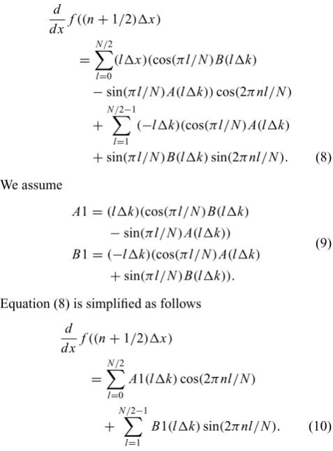
Equation (8) is simplified as follows
d
This is what we are interested in. It can be seen that the staggered grid differentiation (8) or (10) as employing in the PS method can be easily performed by using the real FFT and inverse FFT similarly to the conventional mesh dif-ferentiation. The procedure for the above staggered grid differentiation is summarized as follows. We first obtain the coefficients A(lk)andB(lk)of real data f(n(x)) (n=0,1, . . . ,N−1)according to the formulas (3), (4) and (5). Then we calculate the A1(lk)and B1(lk)coeffi -cients of cosine and sine of (10) according (9). The staggered grid differentiation can be calculated with implementing the real inverse FFT for (8) or (10).
We perform the staggered differentiation (8) or (10) by using the real FFT one third faster than by using the com-plex FFT in (6). So it has lower economic cost to using the differentiation of (10) in PS method. It is obviously seen that the Nyquist coefficient term is also retained (the sec-ond term of the right side of (8)). It is nonzero, equal to
(−π/x)A(k N/2). So the stability of the differentiation of (8) by using real FFT is same as that by using the complex FFT in (6).
5.
Comparison for Real FFT Staggered Operator
and Cagniard-De Hoop Method
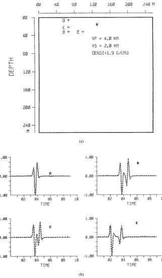
To demonstrate the accuracy of the algorithm presented in this analysis, we compared the calculation result by the real valued FFT differential operators in the staggered grid system presented in the analysis with the result from the ana-lytic result of Cagniard-De Hoop method (Aki and Richards, 1980) for a 2-DS Hproblem in half space with a line source as shown in Fig. 2(a). Figure 2(a) shows a homogenous half space model. The source directional force acting in the ydirection is taken as a Gaussian shape with a Ricker wavelet source time function having a peak frequency of 25 Hz. The time step is 0.001 seconds. In the numerical sim-ulation the 2-D model is sampled with 128×128 points at 20 m spacing in both horizontal and vertical directions. The absorbing boundary condition (Cerjan et al., 1985) is ap-plied on the lateral and bottom edges of the spatial grid in treating the boundary condition. The free-surface condition is approximated by including N-points zero shear velocity above the upper surface of the model in vertical derivatives of stress. The symmetric differentiation method by Furumura and Takenaka (1992) is applied for vertical differentiation of displacement to stabilize the derivatives near the surface nodes. Locations B, C, D and E in Fig. 2(a) are receivers. We will demonstrate calculated waveforms at those locations by the RFFT staggered differentiation method with that cal-culated by the analytic Caganiard-De Hoop method. Fig-ure 2(b) shows the waveform comparisons between results from the above two different methods. Waveforms obtained from RFFT staggered differentiation method (solid circles) and from Cagnard-De Hoop method (thin solid line) are all coincide well for location B, C, D and E, especially in thefirst direct phase. The difference can almost not be distinguished in the waveforms. Small difference can be seen between the two kinds of waveforms in the later reflection phase from surface (somewhat easily seeing in case at point B). Results in Fig. 1(b) suggest that accuracy of the real valued FFT dif-ferential technique in staggered system is comparable with the Cagniard-De Hoop technique. The accuracy of the RFFT staggered differentiation operator in the staggered system is satisfactory.
6.
Example
(a)
(b)
Fig. 2. Comparisons for waveforms calculated from the real valued FFT differential operator in the staggered system presented by this analysis and the Cagniard-De Hoop method. a) Half space homogeneous model for a 2-DS Hproblem; asterisk for line source; B, C, D and E are receivers. b) Waveform comparisons; solid circles for the waveform calculated from the RFFT staggered differentiation method by this paper; thin solid line for waveform from the Cagniard-De Hoop method. The unit of time is 0.1 seconds.
time function (Harrmann, 1979) having 0.4 seconds width with a spatial Guassian shape is used in the analysis taking as the source function. The surface condition and boundary condition in calculation schemes are treated similarly as those used in Section 5.
Figure 3 shows the simulated snapshots at time from 2.0 to 5.0 seconds too. The shots clearly show the propagation
Fig. 3. Heterogeneous velocity structure model with a thrust fault having thrust angle of 45 degrees and snapshots of simulation. Thickness of region I is 2 km. Surface node of the fault plane is 6 km away from the left end corresponding to the 120th grid in Fig. 4. The velocity ofSwave and the density are 1000 m/s and 2.1 g/cm3in the region I, 2000 m/s and 2.5 g/cm3in the region II, respectively. The asterisk for the line source.
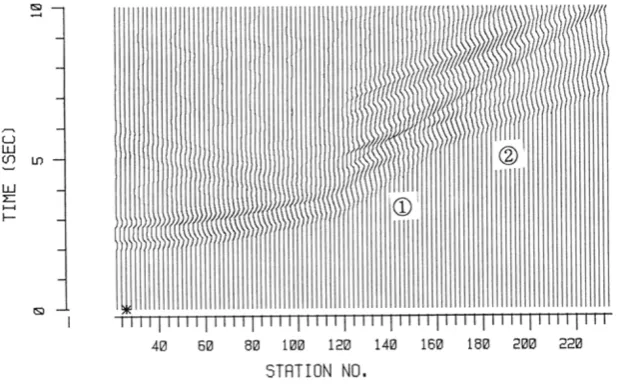
Fig. 4. The waveforms at sites on the surface in Fig. 3. Abscissa for number of stations (record sites), their distances away from the left end are equal to the station number multiplying by the grid spacing of 50 m.1 for the body wave phase,2 for the secondly surface wave phase.
in region II arrives at the free surface of region II fast and is reflected at the surface (seeing the left surface in Fig. 3). We can also see that the wave passes through the fault plane, enters the region I in the shot of 3.0 seconds and propagates along the horizontal direction in region I (seeing shots of 4.0 and 5.0 seconds). We called the wave propagating along horizontal layer (region I) as the secondly surface wave here. The secondly surface wave arrives in the left surface of region I before the upward waves do (seeing the shot of 4.0 seconds). The interference formed of the upward body wave phase and the secondly surface wave propagating along the surface from region II to region I can be seen at the shots of 4.0 and 5.0 seconds. The interference can usually result in the peak of the ground motion that causes large seismic mitigation (Zhao and Kubota, 1997). Irikura et al.(1999) collected some reports on wave interference in the ground motion. Pitarkaet al.(1998) and Kawaseet al.(1998) also reported
the relationship between the peak ground motion and the secondly surface wave in the simulations of the 1995 Hyogo-ken Nanbu earthquake by the FD method. We also can see that the reflected wave from the surface in region II then enters region I along the fault plane and the bottom of region I.
is equal to 1.0 km/s, the same as that of region I in Fig. 3. The phase may be the second surface wave propagating along the layer I in Fig. 3 as mentioned above. The traveltime curve picked from thefirst arrivals for the site number larger than 160 gets even (around region of symbol2), the velocity of wave gets fast. The velocity is near 2.0 km/s which is the apparent velocity of the upward waves with plane wavefront (seeing shots of 4.0 and 5.0 seconds in Fig. 3). Some later phases also can be seen in the waveforms in Fig. 4.
7.
Discussion and Conclusion
We introduced a calculation strategy of the staggered grid differentiation by using the real value FFT and inverse FFT for the PS method of the seismic wave propagation in the present analysis. The calculation by using the RFFT stag-gered differentiation method is one third faster than that by using the traditional complex FFT in the staggered meshed scheme. The Nyquist coefficient term is also retained, and the differentiation is more stable. The differentiation cal-culation strategy introduced in the present analysis is very efficient in economy. In the example for simulation ofS H
wave propagation, we can clearly see the direct wave and reflected wave in region II in Figs. 3 and 4. In the low ve-locity region I we can clearly observe the two transmitting waves, the secondly surface wave from the thrust fault plane and the upward body wave from the bottom of region I. The phenomena mentioned above can also be identified in the snapshots in Fig. 3. The results in Figs. 3 and 4 suggest that the RFFT staggered differentiation operator for the PS method is applicable for seismic simulation.
The differential operators in the staggered grid system by using real valued FFT presented in the analysis is already applied to a 2-DS Hproblem. We think that the RFFT stag-gered differentiation operator can also be extended to more complete wave propagation systems in 2-D or 3-D problem as an effective method.
Acknowledgments. The authors are very grateful to the two anony-mous reviewers for their valuable comments to improve this paper. We also express our heartfelt thanks to professor M. Kikuchi in Uni-versity of Tokyo for the helpful suggestions and comments. This study isfinancially supported by the research projects 2000444 and 2000445 of Ministry of Land and Source of China.
References
Aki, K. and P. G. Richards, Quantitative seismology theory and methods, pp. 224–243, W. H. Freeman and Company, San Francisco, U.S.A., 1980.
Cerjan, C., D. Kosloff, R. Kosloff, and M. Reshef, A nonreflecting boundary condition for discrete acoustic and elastic wave equation,Geophysics,50, 705–708, 1985.
Chen, H. W., Staggered grid pseudospectral simulation in viscoacoustic wavefield simulation,J. Acoust. Soc. Am.,100, 120–131, 1996. Fornberg, B., The pseudospectral method: Comparisons withfinite
differ-ence for the elastic wave equation,Geophysics,52, 483–501, 1987. Furumura, T. and H. Takenaka, A stable method for numerical
differen-tiation of data with discontinuities at end-points by means of fourier transform-symmetric differentiation,Geophys. Expl.,45, 303–309, 1992 (in Japanese).
Furumura, T., B. L. N. Kennett, and H. Takenaka, Parallel 3-D pseudospec-tral simulation of seismic wave propagation,Geophysics,63, 279–288, 1998.
Herrmann, R. B., SH-wave generation by dislocation sources—A numerical study,BSSA,69, 1–15, 1979.
Irikura, K., K. Kudo, H. Okada, and T. Sasatani, The effect of surface geology on seismic motion, in Chap. 3, simultaneous simulation of Kobe, A.A. Balkema, 1594 pp., Rotterdam Press, Netherlands, 1999. Kawase, H., S. Matsushima, R. W. Graves, and P. G. Somervelle,
Three-dimensional wave propagation—The cause of the damage belt during the 1995 Hyogo-ken Nanbu earthquake,Zishin,50, 431–449, 1998. Kosloff, R. and E. Baysal, Forward modeling by a Fourier method,
Geo-physics,42, 1402–1412, 1982.
Orszag, S. A., Comparison of pseudospectral and spectral approximation,
Stud. Appl. Math.,51, 253–259, 1972.
Ozdenvar, T. and G. A. McMechan, Causes and reduction of numerical artefacts in pseudo-spectral wavefield extrapolation,Geophys. J. Int.,126, 819–828, 1996.
Pitarka, A., K. Irikura, T. Iwata, and H. Sekikuchi, Three-dimensional sim-ulation of the near-fault ground motion for the 1995 Hyogo-ken Nanbu (Kobe), Japan, earthquake,BSSA,88, 428–440, 1998.
Reshef, M., D. Kosloff, M. Edwards, and C. Hsiung, Three-dimensional elastic modeling by the Fourier method, Geophysics,53, 1184–1193, 1988.
Saatcilar, R. and S. Ergintav, Solving elastic wave equations with the Hartley method,Geophysics,56, 247–278, 1991.
Virieux, J., SH wave propagation in heterogeneous media: velocity-stress finite difference method,Geophysics,49, 1933–1957, 1984.
Virieux, J., p-sv wave propagation in heterogeneous media: velocity-stress finite-difference method,Geophysics,51, 889–901, 1986.
Witte, D. C., The pseudospectral method for simulating wave propagation, Doctor Thesis, Columbia University, 29 pp., 1989.
Zhao, Z.-X. and R. Kubota, The distribution of strong ground motion from uppermost crustal structure-comparison with disaster from the Hyogo-ken nanbu earthquake, Proceeding of the 97th SEGJ Conference 71– 74, The Society of Exploration Geophysicists of Japan, October, 1997, Sapporo, Japan, 1997.
Zhao, Z.-X. and R. Kubota, The empirical Green’s function method by using simulated waveforms, inThe Effect of Surface geology on Seismic Motion-Recent Progress and New Horizon on ESG Study, Volume 3, edited by K. Irikura, K. Kudo, H. Okata, and T. Sasatani, pp. 1435–1442, A.A. Balkema, Rotterdam Press, Netherlands, 1999.
Zhou, B., On the use of the Hartley transform in geophysical applications,
Geophysics,57, 196–197, 1992.