Indoor robot path planning assisted by wireless network

R E S E A R C H

Open Access

Indoor robot path planning assisted

by wireless network

Xiaohua Wang

, Tengteng Nie

and Daixian Zhu

Abstract

Indoor robot global path planning needs to complete the motion between the starting point and the target point according to robot position command transmitted by the wireless network. Behavior dynamics and rolling windows in global path planning methods have limitations in their applications because the path may not be optimal, there could be a pseudo attractor or blind search in an environment with a large state space, there could be an environment where offline learning is not applicable to real-time changes, or there could be a need to set the probability of selecting the robot action. To solve these problems, we propose a behavior dynamics and rolling windows approach to a path planning which is based on online reinforcement learning. It applies Q learning to optimize the behavior dynamics model parameters to improve the performance, behavior dynamics guides the learning process of Q learning and improves learning efficiency, and each round of intensive learning action selection knowledge is gradually corrected as the Q table is updated. The learning process is optimized. The simulation results show that this method has achieved remarkable improvement in path planning. And, in the actual experiment, the robot obtains the target location information by wireless network, and plans an optimized and smooth global path online.

Keywords:Behavior dynamics, Rolling windows, Q learning, Path planning

1 Introduction

Autonomous navigation in an unknown environment should require that the robot finds a suitable, safe, smooth, and even optimal path from the starting point (position and attitude) to the end point (position and at-titude). Researchers have performed a large amount of research, using artificial neural networks [1],ant colony algorithm[2], and so on combined with fuzzy logic to achieve understanding and rapid classification of current environmental perceptions, the artificial potential field method [3], behavior dynamics [4], Firefly algorithm [5], full coverage path planning algorithm [6], lidar acquisi-tion data and RBPF-SLAM [7] to construct maps, and other methods to solve the autonomous navigation problem in unknown environments for global planning of the robot path or for a combination of global and local planning [8–10]. Researchers combine behavior dy-namics and rolling windows to perform path planning

[11, 12]; the local sub-objective is optimized by using a heuristic function according to the local information in the rolling window obtained by the robot; the behavior dynamics model is used to perform autonomous path planning [13] in the rolling windows; and the planning trajectory of a series of windows is connected end to end to realize the global path planning. Behavior dynamics uses point attractor and point repulsor to build robot behavior, and the robot’s heading angle and motion speed are used as behavior variables to describe robots moving in a plane [14], but in the application, the line speed is limited by the heading angular velocity con-trol and causes a deadlock; in addition, because of the non additivity of the virtual forces, there are also pseudo attractor problems. The literature [15,16] uses the linear velocity control method to solve this problem, but it is required that the linear velocity ensures that the robot’s heading angle is always near the heading angle of the attractor. At the same time, there is also a situation in which the path between windows in the rolling windows method is not smooth because of the different directions of the robot motion.

© The Author(s). 2019Open AccessThis article is distributed under the terms of the Creative Commons Attribution 4.0 International License (http://creativecommons.org/licenses/by/4.0/), which permits unrestricted use, distribution, and reproduction in any medium, provided you give appropriate credit to the original author(s) and the source, provide a link to the Creative Commons license, and indicate if changes were made.

* Correspondence:[email protected]

1_{College of Electrics and Information, Xi’an Polytechnic University, Xi’an,}

China

Reinforcement learning is a machine learning algo-rithm that adjusts its own action strategy by interacting with the environment and ultimately finds the optimal strategy to achieve the goal. The adaptive navigation and obstacle avoidance algorithm based on reinforcement learning can solve the abovementioned problems well and has strong adaptive ability. However, the intensive learning method takes too long to train, and the conver-gence is slow. The general idea of the application of reinforcement learning in robot path planning is as follows [17]: robots roam in the environment, learn obstacle avoidance movements, and gain experience; when robots enter new unknown environments, they rely on previously learned experience to plan obstacle avoidance paths. This kind of approach which involves blind search makes the target reward and punishment spread very slowly, so it is almost impossible to solve the problem of robot navigation in the complex environ-ment with a large state space; in addition, the offline learning method does not apply to the real-time chan-ging environment. Researchers optimize from the aspect of reducing the state space, the action selection, and so on, but they have lost useful information, so the learning cannot be adequately optimized. Some scholars intro-duce the theory of hierarchical reinforcement learning, and they decompose complex reinforcement learning problems into sub-problems that are easy to solve. By solving these sub-problems separately, the original reinforcement learning problems are finally solved [18, 19]. It has also been proposed to use neural net-work structures to automate the hierarchical abstrac-tion and learning of problems [20]. The literature [21] has proposed a reinforcement learning method that is based on path knowledge enlightenment, which uses the knowledge gained by online learning to reduce the blindness of the search, but it needs to set the robot action selection probability fictitiously.

Taking the above research methods into consideration, an idea comes to our mind. If the robot can choose the action itself according to the current state and the ex-perience gained in the learning process, it can not only apply knowledge to enhance the learning efficiency but also enhance the robot’s autonomous navigation ability.

Q learning with behavior dynamics and rolling win-dows is proposed in this paper to solve the problems in robot autonomous navigation while applying the above methods. On the one hand, the online knowledge obtained by applying behavior dynamics improves the robot learning efficiency in this window, and it continu-ously corrects the knowledge obtained in the previous window to optimize the subsequent learning process. On the other hand, the Q-learning behavior dynamics model parameters enable the robot to adaptively change the mo-tion scheme online to adapt to the state in the process of

interacting with the environment, thereby obtaining a good running state and planning an optimal path.

This paper is organized as follows. In Section 2, the robot behavior dynamics model and rolling window path planning method is introduced. Q learning algorithm and the parameters of the Q learning algorithm corres-pond to the motion state of the robot are introduced in Section 3. Afterward, behavior dynamics and rolling windows path planning based on Q learning method is proposed in Section 4. Simulation and experiments are implemented to verify the proposed method in Section 5. Section6gives conclusions.

2 Behavior dynamics and rolling window path planning

2.1 Robot behavior dynamic model

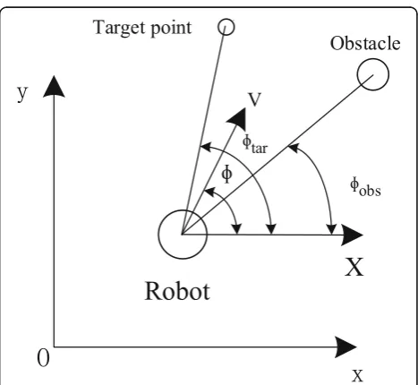
Behavior dynamics uses point attractor and point repul-sor to build robot behavior, and it uses the robot’s head-ing angle and motion speed as the behavior variables to describe robots that move in the plane. The description of the robot and its environment is shown in Fig.1.

The behavior of the robot is determined by both mov-ing toward the target and performmov-ing obstacle avoidance. The behavior dynamics model is coupled by a behavior state dynamics model and a behavior pattern dynamics model. It is a nonlinear differential equation group, and the dynamic state model of robot navigation behavior can be expressed as follows:

φ¼jwtarjftarþjwobsj

X

n

fobsti ð1Þ

whereftaris toward the target behavior function, fobstiis

the obstacle avoidance behavior function, n is the num-ber of obstacles in the environment, and wtar and wobs

are the weights toward the target behavior and the obs-tacle avoidance behavior. This equation constitutes the behavior dynamics model: rameters;α1and α2respectively, represent the competi-tive advantage of the toward the target behavior and the obstacle avoidance behavior; γ12is the coefficient of the constraining ability of the running toward target behav-ior to the obstacle avoidance behavbehav-ior in competition; andγ21is the coefficient of obstacle avoidance behavior’s constraining ability to target behavior in competition. These four parameters describe the extent of coupling between the robot and the environment, and its value changes as the robot’s position changes.

If (wtar,wobs)T= (0, 0)T; then, the fixed points (wtar,

According to Lyapunov’s first approximation theorem [22], as long as the parameters α1, α2, γ12, and γ21 are properly designed so that all of the eigenvalues of the Jacobi matrix that satisfy Eq. (2) have negative real parts, then the fixed point is stable; otherwise, the fixed-point is unstable.

Considering the overall behavior equation of the robot (1), the stability of the above four abovementioned types of fixed points in Eq. (2) can be seen:

1. The first type of fixed point (0, 0) means that the weights of the target behavior and the obstacle avoidance behavior are zero, and both are in the state of complete suppression (i.e., off ), which indicates that the robot is in a roaming disorder state. In the robot navigation process of this paper, this state is not needed. As long asα1> 0 andα2> 0

are satisfied, the fixed point is unstable, and this situation can be avoided.

2. The second type of fixed point (0, ±1) means that in the overall behavior of the robot, there is only obstacle avoidance behavior without target behavior; this situation occurs in the case of robot emergency obstacle avoidance, and as long asy12>

0,α2> 0 is satisfied, this fixed point is stable.

3. The third type of fixed point (±1, 0) means that when there is no obstacle in front of the robot, the robot moves directly to the target point, as long as γ21>α2andα1> 0 are satisfied, the fixed point is a

stable fixed point.

4. The fourth type of fixed point (±A1, ±A2) means

that the weights of the two behavior modes are not 0 or 1 but are between 0 and 1. At this time, both of them act simultaneously,and the navigation behavior of the robot emerges. It is necessary to move to the target while avoiding obstacles and being in a competitive state. Since the parameters α1,α2,γ12, andγ21are descriptions of the coupling

state between the robot and the environment, the value changes as the position of the robot changes. Therefore, the fixed point is changed. The fixed point is stable as long asα1> 0,α2> 0,α1>γ12,

α2>γ21,γ12γ21< 0, orγ12> 0,γ21> 0 are satisfied.

It can be seen from the above stability analysis that the stability of various fixed points is mutually exclusive.-When a fixed point is stable at a certain time, other fixed points are unstable, as long as there are reasonable de-sign parametersα1,α2,γ12,γ21in such a way that the pa-rameters can accurately reflect the relationship between the robot and the environment; then, the correct naviga-tion of the robot can be realized.

In the robot autonomous navigation task, the robot exhibits a mutually coordinated target behavior and obs-tacle avoidance behavior. In interactions with the envir-onment, the robot needs to independently determine the direction and speed of the navigation. The robot’s head-ing angle dynamics model is:

€

system, the distance between the robot and the target point is dt, anddo is the distance between the obstacle

and the robot. The speed dynamics model of the robot is expressed as follows:

whereVexp _tis the desired speed of the target behavior

andVexp _ois the desired speed of the obstacle avoidance

behavior.

2.2 Rolling window path planning

The rolling window path planning method is to use the local environment information acquired by the sensor in real time near the current position of the robot and to perform local path planning under each sub-window to realize the robot behavior control. As the robot advances, the sub-window scrolls forward. This kind of repeated scrolling window local planning realizes a com-bination of optimization and feedback to complete the global planning [23].

The robot acquires environmental information within a certain range of its current location. Regarding this en-vironment as a window, the heuristic function is used to determine the local sub-target point of the window based on the location of the feature point and the obs-tacle. Starting from the current position, the path to reaching the local sub-goal is planned. During the entire navigation process, the window is scrolled forward accordingly, and the prior information in the local envir-onment is corrected. To determine the sub-objects in the window is the premise of the local path planning. The sub-objectives are usually judged by a heuristic function. The heuristic function in this paper is as follows [16]:

F Pð Þ ¼G Pð Þ þH Pð Þ þJ Pð Þ ð5Þ

The G(P) value represents the distance from the sub-target in the setPto the global target guide pointG, and the setPalways guarantees that the sub-target exists in the window.H(P) is the cost ofPto travel to the glo-bal target guidance point, ensuring that the sub-target will not be located in the robot forbidden zone of exist-ing obstacles;J(P) guarantees that the sub-targets of two adjacent windows at momentiand momenti−1 are dif-ferent. The point at whichF(P) is the minimum must be included in the point set at whichH(P) andJ(P) are sim-ultaneously minimized, and if the point at whichG(P) is minimized is also selected at the point set, then the sub-target point of this window is ascertained. The loca-tion of the global target guidance point is the main fac-tor that determines the target of each window. The sub-target point determined by the heuristic function is always close to the global target guidance point.

In each window, the experience acquired by the robot does not form the knowledge of applying subsequent navigation behavior, which results in problems such as the path of the robot’s window junction place not being smooth and the path not being optimal.

3 Q learning algorithm

3.1 Original Q learning algorithm

Most reinforcement learning systems apply a theoretical framework of the Markov decision process (MDP) [24].

The MDP includes the following four parts:S is the en-vironmental state set, A is the set of actions, W:S×

A→T(A) is the set of environmental state transitions, and R:S×A→Ris the feedback signal of the environ-ment state to action which is also a reward value. At

each time t moment, robot obtains an environmental

statestand executes a corresponding actionataccording to a certain strategy, and then, the environment state changes according to the action. At the next moment, robot receives the reward value rt+ 1 from the environ-mental state; that is, for each group given (s,a), here is a reward value Ras; at the same time, robot moves to new environment statest+ 1, and the transition probability is

pa

s. In this learning process, experience knowledge (st,

at, st + 1,at + 1) is obtained. Based on this empirical know-ledge, the Q(s,a) value is modified. Robot’s goal is to

seek in each discrete state S such that Q(s,a) is maximal.

The Q learning algorithm is as follows: InitializationQ(s,a)

For each round of learning { Selection status S = source;

While (Does not satisfy the end condition)

In the current states, we select the behaviora accord-ing to a certain strategy;

Performing actiona, obtaining rewardr, entering state

st+ 1, and updating theQvalue:

Among these, 0 <γ< 1 is called a discount coefficient andβis called a learning rate.

In Q learning, the robot selection action is usually ran-dom or blind. In the single-step reinforcement learning process, the reward obtained after searching for the tar-get can only be propagated one step in the next round, and most of the experience results gained in each round of the search is lost and not fully utilized.

3.2 Q learning about robot

the specified angle in a timely manner according to the angle between the robot and the obstacles.When the robot is farther away from the obstacles, it will acceler-ate or turn the specified angle in a timely manner. Therefore, determining the reward function needs to consider two factors: the distance and angle. The value of the reward function for different distances and angles should be different, specifically as follows:

r¼

tance that the robot has traveled at this moment relative to the previous moment.

Since the robot system does not satisfy the constraint conditions that the state/action must be finite discrete in the Q learning algorithm, there is a need for generalization. In this paper, the neural network is applied to generalize the Q learning algorithm [25]; because the value of the kin-etic parameter is a real number between zero and one, we take 0.2 as the opening degree, and the state-discrete is expressed as s= {s1, s2,s3,s4,s5}, where 0 <s1≤0.2, and so on, 0.8 <s5≤1. The input of the back propagation (BP) net-work corresponds to the five discrete states of the behavior dynamics parameters.The output of the BP network corre-sponds to the Q value of each turning angle action, and there are seven output values in total.

4 Path planning of behavior dynamics and rolling window based on Q learning

4.1 Q learning action search

Original Q learning usually follows certain rules and selects actions, and the choice of actions is random, which results in decreasing the convergence speed of the learning. Applying behavior dynamics knowledge in the rolling window to guide Q learning can reduce the search space and improve the learning efficiency. At the same time, Q learning adjusts the behavior dy-namics parameters in such a way that the robot can better adjust its own running status based on the en-vironmental information.

The Q learning set of actions in this paper is the robot turning angle. The behavior dynamics model also calcu-lates the robot’s heading angle at any time.The current heading angle of the robot is used to guide the Q learn-ing search for the action space to reduce the search scope. The current heading angle of the robot is recorded as A; this angle corresponds to the action space B, and the two discrete action ranges on the left and right, which are similar to this angle, are taken as possible performing actions of the robot, thereby shrink-ing the action space. The probability of execution of each robot action is:

This equation indicates the probability of selecting actionifromjactions in states.

4.2 Shortest path guided robot action selection

In each scroll window, the robot is learning while mov-ing to the sub-target point as the termination condition. The action of the robot is initially calculated by the be-havior dynamics model; with the gradual establishment of theQvalue table, in a certain states, the environmen-tal state also corresponds to a certain action. At this point, there are two possibilities for the robot action. One option is to select the action based on the size of the Q value, and the other option is to use the angle action calculated from formula (3).

This paper is based on the principle in favor of gaining the global shortest path, and it uses the shortest path to determine the robot’s choice of action. At momentt, the robot obtains an environmental statestthat corresponds to the parameters of the behavior dynamics, calculates the distance between the robot and the end point when the robot moves to a new location according to this par-ameter, and calculates the distance between the robot and the end point when the robot that executes the cor-responding actionatreaches the new position according to the Q learning strategy; then, the robot selects an action according to the short distance between the two distances, and at the same time, the Q value table is updated. If the robot performs actions according to the behavior dynamics parameters, this parameter is com-pared to the corresponding state value in the Q value table; then it obtain rewards and updates the Q value table. If the robot performs actions according to the Q learning strategy, theQvalue table is directly updated.

4.3 Q learning knowledge acquisition

One round of learning of the robot will gain some ex-perience, retain the result of this exex-perience, and be able to optimize the later learning process. This paper uses the value of the reward function to make the knowledge in the previous round of learning be applied.

function becomes 2r; that is, each round of know-ledge gained strengthens the learning of the later round. In the process of the robot running, after a series of Q learning, it gradually establishes the Q

value that corresponds to the action knowledge, which is used to guide the Q learning, and it also constantly perfects the knowledge itself. Q learning improved the behavior dynamics parameters, and the interaction between the robot and the environment was significantly improved.

(a)

(b)

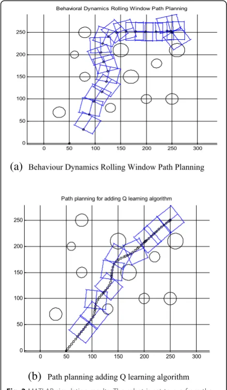
Fig. 2MATLAB simulation results. The robot is set to run from the origin (50, 0) to the endpoint (250, 250), and the maximum speed does not exceed 2 m/s. There are multiple obstacles of different sizes in the environment. The size of the rectangular window is 40 × 34. In the scroll window, the small“。”indicates the position of the robot and forms the robot’s movement trajectory.a, bThe same environment, inbrobot can walk from small space to target point. This result show that Behavior Dynamics Rolling Window Path Planning adding Q learning algorithm is much suitable than Behavior Dynamics Rolling Window Path Planning

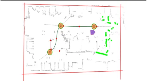
Fig. 3Running track. The trajectory in this figure is the trajectory of the robot in Fig.2b when Q learning method is applied in path planning

(a)

(b)

4.4 Path planning based on Q learning

Based on the above definition of the environment state space, action definition, action search method, action selection, and design of reward function, the path plan-ning step of the behavior dynamics rolling window based on Q learning proposed in this paper is as follows:

Step 1: System initialization; the robot detects the first child window and determines sub-goals.

Step 2: The robot moves in the child window accord-ing to the behavior dynamics model, and it plans the path. The first round of Q learning begins at the same time as the robot movement, and the behavior dynamics model is used to guide the search for Q learning accord-ing to the method of Section3.1; the T table is created.

Step 3: At the starting point of the next window, a new Q learning process is started. A proper reward func-tion value is obtained by querying the table T. The robot performs the action selection according to the method of Section3.2, and the table T is updated.

Step 4: Repeat step 3 until the robot reaches the global end point.

5 Experiments and results analysis

In path planning based on the behavior dynamics model, the position of the obstacles detected by each rolling

window is different, and then, the path walked by the robot is also different. To verify the validity of the above method combination and the continuity and smoothness of the path planning, this paper selects a representative situation in the path planning, and we conduct simula-tion experiments in the MATLAB.

Figure 2a shows the experiment that applies only the behavior dynamics rolling window method. It can be seen from the figure that the robot can avoid the obs-tacle and reach the target point. Figure 2b shows the behavior dynamics rolling window method combined with the Q learning algorithm. In contrast to the path in Fig.2a, the robot can walk in between the obstacles, im-proving the planned path in Fig. 2a and minimizing the path to reach the destination. In the same external envir-onment and exercise conditions, in Fig.2b, the path that the robot can plan is more reasonable than that in figure (a) after applying Q learning algorithm.

The treading track of the robot using Q learning algorithm is shown in Fig.3, and the track shown in Fig.3is smooth. It shows that the Q learning improves the phenomenon that the track is not smooth when the sub-windows are con-nected to each other, making the robot’s kinematic perform-ance perform better in the actual operation.

Figure4is a comparison of robot speeds in the experi-ments shown in Fig.2a and Fig.2b. It can be seen that

the robot speed variation in graph (b) added to the Q learning algorithm is much more moderate than that of graph (a), especially in terms of the distance from the obstacle area after reaching the end point; in graph (b), speed variation trend is obviously better than that of graph (a), which shows that the accumulated know-ledge of Q learning can instruct the robot to better interact with the environment and make the robot move more smoothly.

This method is applied to a real robot system. Mobile R robots carry laser ranging sensor urg-10 lx, accurate Odomete Odomete, gyro module GPX, absolute encoder e6b2-cwz6c 10P/R sensor, and wireless data transmission function circuit module; the wireless data transmission module is used to receive the robot target position infor-mation in the indoor environment, such as point 2 and 3 (Fig. 5). In the process of walking toward the target point (especially from point 1 to point 2), the robot can plan a reasonable route and walk a smooth trajectory. The experimental results show that the proposed method can improve the walking performance of the robot and realize the online global path smoothing.

6 Conclusions

In this paper, the online Q learning method is used to solve the accuracy problem that exists in the robot behavior dynamics model and the problem of the Not smooth path of the rolling window connection. The behavior dynamic model guided Q learning reduced the search space and improved the learning efficiency. The experience and knowledge accumulated in the previous window are beneficial to the later learning; the gradually improved Q learning online adjusts the model parame-ters in such a way that the robot exhibits better performance in interactions with the environment, and an optimized and smooth global path is obtained. This method described in this paper can obtain and use knowledge of the environment in real time, which can improve the practicality of the dynamic model and rolling window path planning and plan an optimal path safely and stably.

Abbreviations

BP:Back propagation; MDP: Markov decision process; RBPF-SLAM: Rao-Blackwellized particle filter (RBPF)-simultaneous localization and mapping (SLAM)

Acknowledgements

The research of this paper is supported by the National Natural Science Foundation of China and the project of ministry of education.

Funding

The authors acknowledge the National Natural Science Foundation of China (No.51607133) and Ministry of education of humanities and social science research special tasks (engineering technology personnel training research) (No.18JDGC029).

Availability of data and materials Not applicable.

Authors_’contributions

Xiaohua Wang is the main writer of this paper. She proposed the main idea, deduced the performance of Q learning algorithm completed the simulation, and analyzed the result. Tengteng Nie introduced the Q learning in robot domain. Daixian Zhu deduced the performance of rolling window path planning algorithm completed the simulation, and analyzed the result. All authors read and approved the final manuscript.

Competing interests

The authors declare that they have no competing interests.

Publisher’s Note

Springer Nature remains neutral with regard to jurisdictional claims in published maps and institutional affiliations.

Author details

1

College of Electrics and Information, Xi’an Polytechnic University, Xi’an, China.2_{College of Communication and Information Engineer, Xi’an University} of Science and Technology, Xi’an, China.

Received: 20 February 2019 Accepted: 18 April 2019

References

1. N.H. Singh, K. Thongam, Mobile robot navigation using MLP-BP approaches in dynamic environments. Arab. J. Sci. Eng.43(12), 8013–8028 (2018) 2. W.B. Zhang, X.P. Gong, G.J. Han, Y.T. Zhao, An improved ant Colony

algorithm for path planning in one scenic area with many spots. IEEE ACCESS. Commun.5, 13260_–13269 (2017)

3. J. Borenstein, Y. Koren, Real time obstacle avoidance for fast mobile robots. IEEE Trans. on Systems Man and Cybernetics Commun.19(5), 1179–1187 (1989)

4. A. Philipp, I. Henrik, Behaviour coordination in structured environments. Adv. Robot17, 657–674 (2003)

5. Y. Shao, S.L. Zhu, R.J. Liu, X.C. Zhou, Diversity-guided dynamic step firefly algorithm. Int. J. of Hybrid Inf. Technol9(8), 95–104 (2016)

6. S.S. Mansouri, K. Christoforos, E. Fresk, D. Kominiak, G. Nikolakopoulos, Cooperative coverage path planning for visual inspection. Control Eng. Pract. Commun.74, 118–131 (2018)

7. J. Hyunggi, H.M. Cho, J.S. jin, K. Euntai, Efficient grid-based Rao-Blackwellized particle filter SLAM with interparticle map sharing. IEEE/ASME Transactions on Mechatronics. Commun.23(2), 714–724 (2018)

8. M. Galicki, Real-time constrained trajectory generation of mobile manipulators. Rob. Autom. Syst.78, 49–62 (2016)

9. J. Keller, D. Thakur, M. Likhachev, J. Gallier, V. Kumar, Coordinated path planning for fixed-wing UAS conducting persistent surveillance missions. IEEE Transactions on Automation Science and Engineering, Commun.14(1), 17–24 (2017)

10. P.K. Mohanty, D.R. Parhi, Optimal path planning for a mobile robot using cuckoo search algorithm. J. Exp. Theor. Artif. Intell.28(1–2), 35–52 (2016) 11. C.A. Liu, X.H. Yan, C.Y. Liu, H. Wu, Dynamic path planning for mobile robot

based on improved ant colony optimization algorithm. Acta Electronica sinica.39(5), 1220_–1224 (2011)

12. J.J. TY Zhang, G.X. Zhang,Analysis of a dual-arm mobile robot dynamics and balance compensationInt. J. Comput. Appl. Technol. 41(3–4), 246–252 (2011)

13. L. Zhang, X.J. Zhang, K.H. Guo, C.L. Wang, L. Yang, T. Liu, Rolling window optimization for intelligent vehicle trajectory planning in unknown environment. Journal of Jilin University (Engineering and Technology Edition), Commun.48(3), 652–660 (2018)

14. Y.F. Zhang, W.L. Li, D. Silva, W. Clarence, RSMDP-based robust Q-learning for optimal path planning in a dynamic environment. Int J Rob Autom.31(4), 290–300 (2016)

16. A. Gentile, A. Messina, Dynamic behaviour of a mobile robot vehicle with a two caster and two driving wheel configuration. Veh. Syst. Dyn.25(2), 89_– 112 (1996)

17. H.K. Sajad, B.S. Saeed, S.K. Soroush, Path planning of modular robots on various terrains using Q-learning versus optimization algorithms. Intell. Serv. Robot10(2), 121_–136 (2017)

18. Z.F. Shao, J.E. Meng, A survey of inverse reinforcement learning techniques. International Journal of Intelligent Computing and Cybernetics, Commun 5(3), 293–311 (2012)

19. L.W. Zhou, P. Yang, C.L. Chen, Y. Gao, Multiagent reinforcement learning with sparse interactions by negotiation and knowledge transfer. IEEE Transactions on Cybernetics, Commun.47(5), 1238–1250 (2017) 20. H. Huang, X.T. Hu, Y. Zhao, M. Milad, Q.L. Dong, S.J. Zhao, L. Guo, T.M. Liu,

Modeling task fMRI data via deep convolutional autoencoder. IEEE Transactions on Medical Imaging, Commun.37(7), 1551–1561 (2018) 21. H.P. Zhu, F. Tian, K. Wu, S. Nazaraf, Y. Chen, Y.F. Ni, X.H. Zhang, K.M. Chao, Q.

H. Zheng, A multiconstraint learning path recommendation algorithm based on knowledge map. Knowl. -Based Syst.143, 102_–114 (2018) 22. A.J. Krener, M.Q. Xiao, Nonlinear observer design in the siegel domain. SIAM

J. Control Optim.41(3), 932–953 (2003)

23. L.L. Yu, D.C.H. Kong, X.Y. Shao, X.X. Yan, A path planning and navigation control system design for driver less electric bus. IEEE Access, Commun.6, 53960–53975 (2018)

24. C.H. Jaedeug, K.E. Kim, Inverse reinforcement learning in partially observable environments. J. Mach. Learn. Res.12, 691–730 (2011)