Mark Dredze [email protected]
Koby Crammer [email protected]
Department of Computer and Information Science, University of Pennsylvania, Philadelphia, PA 19104 USA
Fernando Pereira1 [email protected]
Google, Inc., 1600 Amphitheatre Parkway, Mountain View, CA 94043 USA
Abstract
We introduce confidence-weighted linear clas-sifiers, which add parameter confidence infor-mation to linear classifiers. Online learners in this setting update both classifier param-eters and the estimate of their confidence. The particular online algorithms we study here maintain a Gaussian distribution over parameter vectors and update the mean and covariance of the distribution with each in-stance. Empirical evaluation on a range of NLP tasks show that our algorithm improves over other state of the art online and batch methods, learns faster in the online setting, and lends itself to better classifier combina-tion after parallel training.
1. Introduction
Online learning algorithms operate on a single instance at a time, allowing for updates that are fast, simple, make few assumptions about the data, and perform well in wide range of practical settings. Online learn-ing algorithms have become especially popular in nat-ural language processing for tasks including classifica-tion, tagging, and parsing. In this paper, we revisit the design of linear classifier learning informed by the particularities of natural language tasks. Specifically, feature representations for natural language processing have very high dimension (millions of features derived from words and word combinations are common), and most features are observed on only a small fraction of instances. Nevertheless, those many rare features are important in classifying the instances in which they
1
Work done at the University of Pennsylvania.
Appearing inProceedings of the 25thInternational Confer-ence on Machine Learning, Helsinki, Finland, 2008. Copy-right 2008 by the author(s)/owner(s).
occur. Therefore, it is worth investigating whether online learning algorithms for linear classifiers could be improved to take advantage of these particularities of natural language data.
We introduce confidence-weighted (CW) learning, a new class of online learning methods that maintain a probabilistic measure of confidence in each parameter. Less confident parameters are updated more aggres-sively than more confident ones. Parameter confidence is formalized with a Gaussian distribution over param-eter vectors, which is updated for each new training in-stance so that the probability of correct classification for that instance under the updated distribution meets a specified confidence. We show superior classification accuracy over state-of-the-art online and batch base-lines, faster learning, and new classifier combination methods after parallel training.
We begin with a discussion of the motivating particu-larities of natural language data. We then derive our algorithm and discuss variants. A series of experiments shows CW learning’s empirical benefits. We conclude with a discussion of related work.
2. Online Algorithms and NLP
In natural language classification tasks, many differ-ent features, most of which are binary and are infre-quently on, can be weakly indicative of a particular class. Therefore, we have both data sparseness, which demands large training sets, and very high dimen-sional parameter vectors. For certain types of prob-lems, such as structured prediction in tagging or pars-ing, the size and processing complexity of individual instances make it difficult to keep more than a small number of instances in main memory. These particu-larities make online algorithms, which process a single instance at a time, a good match for natural-language tasks. Processing large amounts of data is simple for online methods, which require observing each instance once — though in practice several iterations may be
necessary — and update parameter vectors using a sin-gle instance at a time. In addition, the simple nature of most online updates make them very fast.
However, while online algorithms do well with large numbers of features and instances, they are not de-signed for the heavy tailed feature distributions char-acteristic of natural language tasks. This type of feature distribution can have a detrimental effect on learning. With typical linear classifier training algo-rithms, such as the perceptron or passive-aggressive (PA) algorithms (Rosenblatt, 1958; Crammer et al., 2006), the parameters of binary features are only up-dated when the features occur. Therefore, frequent features typically receive more updates. Similarly, fea-tures that occur early in the data stream take more re-sponsibility for correct prediction than those observed later. The result is a model that could have good pa-rameter estimates for common features and inaccurate values for rare features. However, no distinction is made between these feature types in most online algo-rithms.
Consider an illustrative example from the problem of sentiment classification. In this task, a product review is represented asn-grams and the goal is to label the review as being positive or negative about the prod-uct. Consider a positive review that simply read “I
liked this author.” An online update would increase
the weight of both “liked” and “author.” Since both are common words, over several examples the algo-rithm would converge to the correct values, a positive weight for “liked” and zero weight for “author.” Now consider a slightly modified negative example: “I liked
this author, but found the book dull.” Since “dull”
is a rare feature, the algorithm has a poor estimate of its weight. An update would decrease the weight of both “liked” and “dull.” The algorithm does not know that “dull” is rare and the changed behavior is likely caused by the poorly estimated feature (“dull”) in-stead of the common well estimated feature (“liked.”) This update incorrectly modified “liked” and does not attribute enough negative weight to “dull,” thereby decreasing the rate of convergence.
This example demonstrates how a lack of memory for previous instances — a property that allows online learning — can hurt learning. A simple solution is to augment an online algorithm with additional in-formation, a memory of past examples. Specifically, the algorithm can maintain a confidence parameter for each feature weight. For example, assuming bi-nary features, the algorithm could keep a count of the number of times each feature has been observed, or, for general real-valued features, it could keep the
cu-mulative second moment per feature. The larger the count or second moement, the more confidence in a feature’s weight. These estimates are then used to influence parameter updates. Instead of equally up-dating every feature weight for the features present in an instance, the update favors changing more low-confidence weights than high-low-confidence ones. At each update, the confidence in all observed features is in-creased by focusing the update on low confidence fea-tures. In the example above, the update would de-crease the weight of “dull” but make only a small change to “liked” since the algorithm already has a good estimate of this parameter.
3. Online Learning of Linear Classifiers
Online algorithms operate in rounds. On round ithe algorithm receives an instance xi ∈ Rd to which it
applies its current prediction rule to produce a pre-diction ˆyi ∈ {−1,+1} (for binary classification.) It
then receives the true labelyi ∈ {−1,+1} and suffers
a loss`(yi,yˆi), which in this work will be the zero-one
loss `(yi,yˆi) = 1 if yi = ˆ6 yi and `(yi,yˆi) = 0
other-wise. The algorithm then updates its prediction rule and proceeds to the next round.
Just as in many well known algorithms, such as the perceptron and support vector machines, in this work our prediction rules are linear classifiers
fw(x) :fw(x) = sign(x·w). (1)
If we fix the norm of w, we can identify fw with w,
and we will usew in the rest of this work.
The margin of an example (x, y) with respect to a
specific classifier w is given by y(w ·x). The sign of the margin is positive iff the classifier w predicts correctly the true label y. The absolute value of the margin|y(w·x)| =|w·x|is often thought of as the
confidencein the prediction, with larger positive values corresponding to more confident correct predictions. We denote the margin at roundibymi=yi(wi·xi).
A variety of linear classifier training algorithms, in-cluding the perceptron and linear support vector ma-chines, restrict w to be a linear combination of the input examples. Online algorithms of that kind typi-cally have updates of the form
wi+1=wi+αiyixi , (2)
for some non-negative coefficientsαi.
In this paper we focus on PA updates (Crammer et al., 2006) for linear classifiers. After predicting with wi
algorithm updates the prediction function such that the example (xi, yi) will be classified correctly with a
fixed margin (which can always be scaled to 1):
wi+1= min w 1 2kwi−wk 2 (3) s.t. yi(w·xi)≥1 .
The dual of (3) gives us the round coefficients for (2): αi= max ( 1−yi(wi·xi) kxik2 ,0 )
Crammer et al. (2006) provide a theoretical analysis of algorithms of this form, and they have been shown to work well in a variety of applications.
4. Distributions over Classifiers
We model parameter confidence for a linear classi-fier with a diagonal Gaussian distribution with mean
µ ∈Rd and standard deviation σ ∈ Rd. The values
µj and σj represent our knowledge of and confidence
in the parameter for feature j. The smaller σj, the
more confidence we have in the mean parameter value µj. For simplicity of presentation, we use a covariance
matrix Σ ∈ Rd×d for the distribution, with diagonal
σ and zero for off-diagonal elements. Note that while our motivation assumed sparse binary features, the al-gorithm does not depend on that assumption.
Conceptually, to classify an input instancex, we draw a parameter vectorw∼ N(µ,Σ) and predict the label according to the sign ofw·x. This multivariate Gaus-sian distribution over parameter vectors induces a uni-variate Gaussian distribution over the margin viewed as a random variable:
M ∼ N yi(µ·xi), x>i Σxi
.
The mean of the margin is the margin of the averaged parameter vector and its variance is proportional to the length of the projection ofxi on Σi. Since a
pre-diction is correct iff the margin is non-negative, the probability of a correct prediction is
Prw∼N(µ,Σ)[M ≥0] = Prw∼N(µ,Σ)[yi(w·xi)≥0] .
When possible, we omit the explicit dependency on the distribution parameters and write Pr [yi(w·xi)≥0].
4.1. Update
On roundi, the algorithm adjusts the distribution to ensure that the probability of a correct prediction for training instance i is no smaller than the confidence hyperparameter η∈[0,1]:
Pr [yi(w·xi)≥0]≥η . (4)
Following the intuition underlying the PA algo-rithms (Crammer et al., 2006), our algorithm chooses the distribution closest in the KL divergence sense to the current distributionN(µi,Σi). Thus, on roundi,
the algorithm sets the parameters of the distribution by solving the following optimization problem:
(µi+1,Σi+1) = min DKL(N(µ,Σ)k N(µi,Σi)) (5)
s.t. Pr [yi(w·xi)≥0]≥η . (6)
We now develop both the objective and the constraint of this optimization problem following Boyd and Van-denberghe, (2004, page 158). We start with the con-straint (6). As noted above, under the distribution N(µ,Σ), the margin for (xi, yi) has a Gaussian
dis-tribution with mean µM = yi(µ·xi) and variance
σ2
M =x>i Σxi. Thus the probability of awrong
classi-fication is Pr [M ≤0] = Pr M −µM σM ≤−µM σM .
Since (M −µM)/σM is a normally distributed random
variable, the above probability equals Φ (−µM/σM),
where Φ is the cumulative function of the normal dis-tribution. Thus we can rewrite (6) as
−µM
σM
≤Φ−1(1−η) =−Φ−1(η) .
Substituting µM and σM by their definitions and
re-arranging terms we obtain: yi(µ·xi)≥φ
q
x>i Σxi ,
whereφ= Φ−1(η).
Unfortunately, this constraint is not convex in Σ, so we linearize it by omitting the square root:
yi(µ·xi)≥φ x>i Σxi
. (7)
Conceptually, this is a large-margin constraint, where the value of the margin requirement depends on the examplexivia a quadratic form.
We now study the objective (5). The KL divergence between two Gaussians is given by
DKL(N(µ0,Σ0)k N(µ1,Σ1)) = 1 2 log det Σ 1 det Σ0 + Tr Σ−11Σ0 + (µ1−µ0) > Σ−11(µ1−µ0)−d . (8)
Using the foregoing equations and omitting irrelevant constants, we obtain the following revised optimization problem: (µi+1,Σi+1) = min 1 2log det Σ i det Σ +1 2Tr Σ −1 i Σ +1 2(µi−µ) > Σ−i 1(µi−µ) s.t. yi(µ·xi)≥φ x>i Σxi . (9)
The optimization objective is convex in µ and Σ si-multaneously and the constraint is linear, so any con-vex optimization solver could be used to solve this problem. We call the corresponding update Variance-Exact. However, for efficiency we prefer a closed-form approximate update that we callVariance. In this ap-proximation, we allow the solution for Σi+1 in (9) to produce (implicitly) a full matrix, and then project it to a diagonal matrix, where the non-zero off-diagonal entries are dropped. The Lagrangian for this optimiza-tion is L = 1 2log det Σi det Σ +1 2Tr Σ −1 i Σ +1 2(µi−µ) > Σ−i1(µi−µ) +α −yi(µ·xi) +φ x>i Σxi . (10) At the optimum, we must have
∂ ∂µL= Σ
−1
i (µ−µi)−αyixi= 0 .
Assuming Σi is non-singular we get,
µi+1=µi+αyiΣixi . (11)
At the optimum, we must also have ∂ ∂ΣL=− 1 2Σ −1+1 2Σ −1 i +φαxix>i = 0.
Solving for Σ−1 we obtain
Σ−i+11 = Σi−1+ 2αφxix>i . (12)
Finally, we compute the inverse of (12) using the Woodbury identity (Petersen & Pedersen, 2007, Eq. 135) and get, Σi+1= Σ−i1+ 2αφxix>i −1 = Σi−Σixi 1 2αφ+x > i Σixi −1 x>i Σi = Σi−Σixi 2αφ 1 + 2αφx>i Σixi x>i Σi . (13)
The KKT conditions for the optimization imply that the either α = 0, and no update is needed, or the constraint (7) is an equality after the udpate. Substi-tuting (11) and (13) into the equality version of (7), we obtain: yi(xi·(µi+αyiΣixi)) = φ x>i Σi−Σixi 2αφ 1 + 2αφx>i Σixi x>i Σi xi . (14) Rearranging terms we get,
yi(xi·µi) +αx>i Σixi=
φx>i Σixi−φ x>i Σixi
2 2αφ
1 + 2αφx>i Σixi
. (15) For simplicity, let Mi =yi(xi·µi) be the mean
mar-gin and Vi = x>i Σixi be the margin variance before
the update. Substituting these into (15) we get, Mi+αVi=φVi−φVi2
2αφ 1 + 2αφVi
.
It is straightforward to see that this is a quadratic equation inα. Its smaller root is always negative and thus is not a valid Lagrange multiplier. Let γi be its
larger root: γi= −(1+2φMi)+ q (1+2φMi)2−8φ(Mi−φVi) 4φVi . (16) The constraint (7) is satisfied before the update ifMi−
φVi ≥ 0. If 1 + 2φMi ≤ 0, thenMi ≤φVi and from
(16) we have that γi >0. If, instead, 1 + 2φMi ≥0,
then, again by (16), we have γi>0 ⇔ q (1 + 2φMi) 2 −8φ(Mi−φVi)>(1 + 2φMi) ⇔Mi< φVi .
From the KKT conditions, eitherαi= 0 or (9) is
sat-isfied as an equality. In the later case, (14) holds, and thusαi =γi >0. To summarize, we have proved the
following:
Lemma 1 The optimal value of the Lagrange multi-plier is given byαi= max{γi,0}.
The above derivation yields a full covariance matrix. As noted above, we restrict ourself to diagonal matri-ces and thus we project the solution into the set of diagonal matrices to get our approximation. In prac-tice, it is equivalent to computeαias above but update
with the following rule instead of (12).
Algorithm 1Variance Algorithm (Approximate) Input: confidence parameterφ= Φ−1(η)
initial variance parametera >0 Initialize: µ1=0, Σ1=aI
fori= 1,2. . . do
Receivexi∈Rd ,yi∈ {+1,−1}
Set the following variables: αi as in Lemma 1 µi+1=µi+αiyiΣixi (11) Σ−i+11 = Σ−i1+ 2αiφdiag (xi) (17) end for comp comp.sys.ibm.pc.hardware comp.sys.mac.hardware sci sci.electronics sci.med talk talk.politics.guns talk.politics.mideast
Table 1. 20 Newsgroups binary decision tasks.
where diag (xi) is a diagonal matrix with the square
of the elements ofxi on the diagonal.
The pesudocode of the algorithm appears in Alg. 1. From the initalization of Σ1 and the update rule of (12), we conclude that the eigenvalues of Σi are
shirinking, but never set to zero explicltly, and thus the covariance matrices Σi are not singular.
5. Evaluation
We evaluated our Variance and Variance-Exact algo-rithms on three popular NLP datasets. Each dataset contains several binary classification tasks from which we selected a total of 12 problems, each contains a balanced mixture of instance labels.
20 Newsgroups The 20 Newsgroups corpus con-tains approximately 20,000 newsgroup messages, par-titioned across 20 different newsgroups.2 The dataset is a popular choice for binary and multi-class text clas-sification as well as unsupervised clustering. Following common practice, we created binary problems from the dataset by creating binary decision problems of choosing between two similar groups, as shown in Ta-ble 1. Each message was represented as a binary bag-of-words. For each problem we selected 1800 instances. Reuters The Reuters Corpus Volume 1 (RCV1-v2/LYRL2004) contains over 800,000 manually catego-rized newswire stories (Lewis et al., 2004). Each article
2
http://people.csail.mit.edu/jrennie/20Newsgroups/
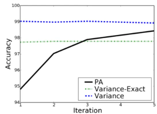
Figure 1.Accuracy on test data after each iteration on the
“talk” dataset.
contains one or more labels describing its general topic, industry and region. We created the following binary decision tasks from the labeled documents: Insurance: Life (I82002) vs. Non-Life (I82003), Business Services: Banking (I81000) vs. Financial (I83000), and Retail Distribution: Specialist Stores (I65400) vs. Mixed Re-tail (I65600). These distinctions involve neighboring categories so they are fairly hard to make. Details on document preparation and feature extraction are given by Lewis et al. (2004). For each problem we selected 2000 instances using a bag of words represen-tation with binary features.
Sentiment We obtained a larger version of the sen-timent multi-domain dataset of Blitzer et al. (2007) containing product reviews from 6 Amazon domains (book, dvd, electronics, kitchen, music, video). The goal in each domain is to classify a product review as either positive or negative. Feature extraction follows Blitzer et al. (2007). For each problem we selected 2000 instances using uni/bi-grams with counts. Each dataset was randomly divided for 10-fold cross validation experiments. Classifier parameters (φ for CW andC for PA) were tuned for each classification task on a single randomized run over the data. Results are reported for each problem as the average accuracy over the 10 folds. Statistical significance is computed using McNemar’s test.
5.1. Results
We start by examining the performance of the Vari-ance and VariVari-ance-Exact versions of our method, dis-cussed in the preceding section, against a PA algo-rithm. All three algorithms were run on the datasets described above and each training phase consisted of five passes over the training data, which seemed to be
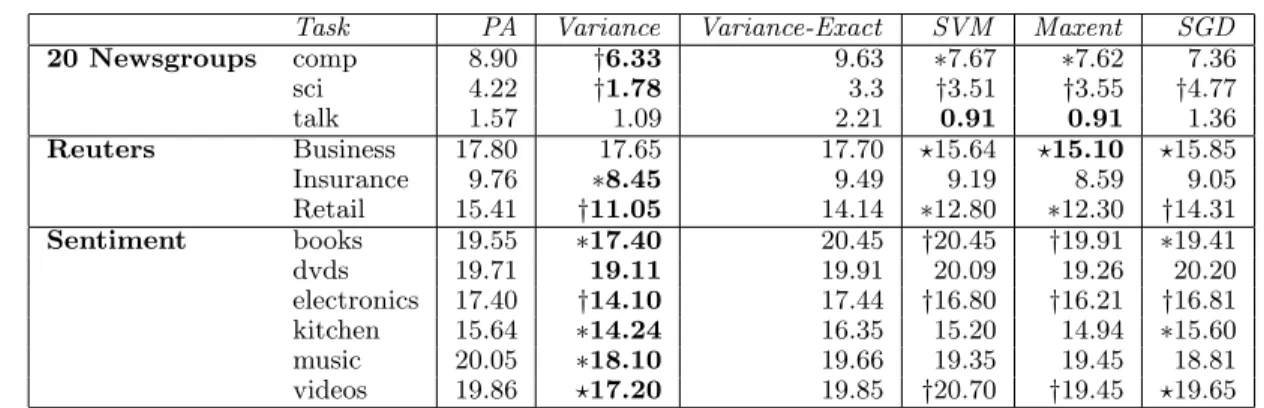
Task PA Variance Variance-Exact SVM Maxent SGD 20 Newsgroups comp 8.90 †6.33 9.63 ∗7.67 ∗7.62 7.36 sci 4.22 †1.78 3.3 †3.51 †3.55 †4.77 talk 1.57 1.09 2.21 0.91 0.91 1.36 Reuters Business 17.80 17.65 17.70 ?15.64 ?15.10 ?15.85 Insurance 9.76 ∗8.45 9.49 9.19 8.59 9.05 Retail 15.41 †11.05 14.14 ∗12.80 ∗12.30 †14.31 Sentiment books 19.55 ∗17.40 20.45 †20.45 †19.91 ∗19.41 dvds 19.71 19.11 19.91 20.09 19.26 20.20 electronics 17.40 †14.10 17.44 †16.80 †16.21 †16.81 kitchen 15.64 ∗14.24 16.35 15.20 14.94 ∗15.60 music 20.05 ∗18.10 19.66 19.35 19.45 18.81 videos 19.86 ?17.20 19.85 †20.70 †19.45 ?19.65
Table 2.Error on test data using batch training. Statistical significance (McNemar) is measured against PA or the batch
method against Variance. (∗p=.05,?p=.01,†p=.001)
enough to yield convergence. The average error on the test set for the three algorithms on all twelve datasets is shown in table 2.
Variance-Exact achieved about the same performance as PA, with each method achieving a lower error on half of the datasets. In contrast, Variance (approxi-mate) significantly improves over PA, achieving lower error on all twelve datasets, with statistically signifi-cant results on nine of them.
As discussed above, online algorithms are attractive even for batch learning because of their simplicity and ability to operate on extremely large datasets. In the batch setting, these algorithms are run several times over the training data, which yields slower per-formance than single pass learning (Carvalho & Co-hen, 2006). Our algorithm improves on both accuracy and learning speed by requiring fewer iterations over the training data. Such behavior can be seen on the “talk” dataset in Figure 1, which shows accuracy on test data after each iteration of the PA baseline and the two variance algorithms. While Variance clearly improves over PA, it converges very quickly, reaching near best performance on the first iteration. In con-trast, PA benefits from multiple iterations over the data; its performance changes significantly from the first to fifth iteration. Across the twelve tasks, Vari-ance yields a 3.7% error reduction while PA gives a 12.4% reduction between the first and fifth iteration, indicating that multiple iterations help PA more. The plot also illustrates Variance-Exact’s behavior, which initially beats PA but does not improve. In fact, on eleven of the twelve datasets, Variance-Exact beats PA on the first iteration. The exact update results in ag-gressive behavior causing the algorithm to converge very quickly, even more so than Variance. It appears that the approximate update in Variance reduces over-training and yields the best accuracy.
10 50 100 Number of Parallel Classifiers 90 91 92 93 94 95 96 Test Accuracy Reuters 10 50 100 Number of Parallel Classifiers 90 91 92 93 94 95 96 Test Accuracy Sentiment Average Uniform Weighted PA Variance
Figure 2.Results for Reuters (800k) and Sentiment
(1000k) averaged over 4 runs. Horizontal lines show the test accuracy of a model trained on the entire training set. Vertical bars show the performance ofn(10, 50, 100) clas-sifiers trained on disjoint sections of the data as the average performance, uniform combination, or weighted combina-tion. All improvements are statistically significant except between uniform and weighted for Reuters.
5.2. Batch Learning
While online algorithms are widely used, batch algo-rithms are still preferred for many tasks. Batch al-gorithms can make global learning decisions by exam-ining the entire dataset, an ability beyond online al-gorithms. In general, when batch algorithms can be applied they perform better. We compare our new on-line algorithm (Variance) against two standard batch algorithms: maxent classification (default configura-tion of the maxent learner in McCallum (2002)) and support vector machines (LibSVM (Chang & Lin, 2001)). We also include stochastic gradient descent (SGD) (Blitzer et al., 2007), which performs well for NLP tasks. Classifier parameters (Gaussian prior for maxent, C for SVM and the learning rate for SGD) were tuned as for the online methods.
Results for batch learning are shown in Table 2. As ex-pected, the batch methods tend to do better than PA,
with SVM doing better 9 times and maxent 11 times. However, in most cases Variance improves over the batch method, doing better than SVM and maxent 10 out of 12 times (7 statistically significant.) These re-sults show that in these tasks, the much faster and sim-pler online algorithm performs better than the slower more complex batch methods.
We also evaluated the effects of commonly used tech-niques for online and batch learning, including aver-aging and TFIDF features, none of which improved accuracy. Although the above datasets are balanced with respect to labels and predictive features, we also evaluated the methods on variant datasets with un-balanced label or feature distributions, and still saw similar benefits from the Variance method.
5.3. Large Datasets
Online algorithms are especially attractive in tasks where training data exceeds available main memory. However, even a single sequential pass over the data can be impractical for extremely large training sets, so we investigate training different models on differ-ent portions of the data in parallel and combining the learned classifiers into a single classifier. While this of-ten does not perform as well as a single model trained on all of the data, it is a cost effective way of learning from very large training sets.
Averaging models trained in parallel assumes that each model has an equally accurate estimate of the model parameters. However, our model provides a confidence value for each parameter, allowing for a more intelli-gent combination of parameters from multiple models. Specifically, we compute the combined model Gaus-sian that minimizes the total divergence to the setC of individually trained classifiers for some divergence operatorD: min µ,Σ X c∈C D((µ,Σ)||(µc,Σc)), (18)
IfDis the Euclidean distance, this is just the average of the individual models. If D is the KL divergence, the minimization leads to the following weighted com-bination of individual model means:
µ= P c∈CΣ− 1 c −1P c∈CΣ− 1 c µc, Σ− 1=P c∈CΣ− 1 c .
We evaluate the single model performance of the PA baseline and our method. For our method, we evaluate classifier combination by trainingn(10, 50, 100) mod-els by dividing the instance stream intondisjoint parts and report the average performance of each of the n classifiers (average), the combined classifier from tak-ing the average of then sets of parameters (uniform) and the combination using the KL distance (weighted)
on the test data across 4 randomized runs.
We evaluated classifier combination on two datasets. The combined product reviews for all the domains in Blitzer et al. (2007) yield one million sentiment instances. While most reviews were from the book do-main, the reviews are taken from a wide range of Ama-zon product types and are mostly positive. From the Reuters corpus, we created a one vs. all classification task for theCorporate topic label, yielding 804,411 in-stances of which 381,325 are labeled corporate. For the two datasets, we created four random splits each with one million training instances and 10,000 test in-stances. Parameters were optimized by training on 5K random instances and testing on 10K.
The two datasets use very different feature representa-tions. The Reuters data contains 288,062 unique fea-tures, for a feature to document ratio of 0.36. In con-trast, the sentiment data contains 13,460,254 unique features, a feature to document ratio of 13.33. This means that Reuters features tend to occur several times during training while many sentiment features occur only once.
Average accuracy on the test sets are reported in Fig-ure 2. For Reuters data, the PA single model achieves higher accuracy than Variance, possibly because of the low feature to document ratio. However, combining 10 Variance classifiers achieves the best performance. For sentiment, combining 10 classifiers beats PA but is not as good as a single Variance model. In every case, com-bining the classifiers using either uniform or weighted improves over each model individually. On sentiment weighted combination improves over uniform combi-nation and in Reuters the models are equivalent. Finally, we computed the actual run time of both PA and Variance on the large datasets to compare the speed of each model. While Variance is more complex, requiring more computation per instance, the actual speed is comparable to PA; in all tests the run time of the two algorithms was indistinguishable.
6. Related Work
The idea of using parameter-specific variable ing rates has a long history in neural-network learn-ing (Sutton, 1992), although we do not know of a previ-ous model that specifically models confidence in a way that takes into account the frequency of features. The second-order perceptron (SOP) (Cesa-Bianchi et al., 2005) is perhaps the closest to our CW algorithm. Both are online algorithms that maintain a weight vector and some statistics about previous examples. While the SOP models certainty with feature counts,
CW learning models uncertainty with a Gaussian dis-tribution. CW algorithms have a probabilistic moti-vation, while the SOP is based on the geometric idea of replacing a ball around the input examples with a refined ellipsoid. Shivaswamy and Jebara (2007) used this intuition in the context of batch learning. Gaussian process classification (GPC) maintains a Gaussian distribution over weight vectors (primal) or over regressor values (dual). Our algorithm uses a dif-ferent update criterion than the the standard Bayesian updates used in GPC (Rasmussen & Williams, 2006, Ch. 3), avoiding the challenging issues in approximat-ing posteriors in GPC. Bayes point machines (Herbrich et al., 2001) maintain a collection of weight vectors consistent with the training data, and use the sin-gle linear classifier which best represents the collec-tion. Conceptually, the collection is a non-parametric distribution over the weight vectors. Its online ver-sion (Harrington et al., 2003) maintains a finite num-ber of weight-vectors updated simultaneously.
Finally, with the growth of available data there is an increasing need for algorithms that process training data very efficiently. A similar approach to ours is to train classifiers incrementally (Bordes & Bottou, 2005). The extreme case is to use each example once, without repetitions, as in the multiplicative update method of Carvalho and Cohen (2006).
Conclusion: We have presented confidence-weighted linear classifiers, a new learning method designed for NLP problems based on the notion of parameter confidence. The algorithm maintains a distribution over parameter vectors; online updates both improve the parameter estimates and reduce the distribution’s variance. Our method improves over both online and batch methods and learns faster on a dozen NLP datasets. Additionally, our new algorithms allow more intelligent classifier combi-nation techniques, yielding improved performance after parallel learning. We plan to explore theoretical properties and other aspects of CW classifiers, such as multi-class and structured prediction tasks, and other data types.
Acknowledgements: This material is based upon work supported by the Defense Advanced Research Projects Agency (DARPA) under Contract No. FA8750-07-D-0185.
References
Blitzer, J., Dredze, M., & Pereira, F. (2007). Biogra-phies, bollywood, boom-boxes and blenders:
Do-main adaptation for sentiment classification.
As-sociation of Computational Linguistics (ACL).
Bordes, A., & Bottou, L. (2005). The huller: a simple and efficient online svm. European Conference on
Machine Learning( ECML ), LNAI 3720.
Boyd, S., & Vandenberghe, L. (2004). Convex
opti-mization. Cambridge University Press.
Carvalho, V. R., & Cohen, W. W. (2006). Single-pass online learning: Performance, voting schemes and online feature selection. KDD-2006.
Cesa-Bianchi, N., Conconi, A., & Gentile, C. (2005). A second-order perceptron algorithm. SIAM Journal on Computing,34, 640 – 668.
Chang, C.-C., & Lin, C.-J. (2001). LIBSVM: a library
for support vector machines. Software available at
http://www.csie.ntu.edu.tw/∼cjlin/libsvm. Crammer, K., Dekel, O., Keshet, J., Shalev-Shwartz,
S., & Singer, Y. (2006). Online passive-aggressive algorithms. JMLR, 7, 551–585.
Harrington, E., Herbrich, R., Kivinen, J., Platt, J., & Williamson, R. (2003). Online bayes point ma-chines. 7th Pacific-Asia Conference on Knowledge
Discovery and Data Mining (PAKDD).
Herbrich, R., Graepel, T., & C.Campbell (2001). Bayes point machinesonline passive-aggressive algo-rithms. JMLR,1, 245–279.
Lewis, D. D., Yand, Y., Rose, T., & Li., F. (2004). Rcv1: A new benchmark collection for text catego-rization research. JMLR,5, 361–397.
McCallum, A. K. (2002). Mallet: A machine learning for language toolkit. http://mallet.cs.umass.edu. Petersen, K. B., & Pedersen, M. S. (2007). The matrix
cookbook.
Rasmussen, C. E., & Williams, C. K. I. (2006). Gaus-sian processes for machine learning. The MIT Press. Rosenblatt, F. (1958). The perceptron: A probabilistic model for information storage and organization in the brain. Psych. Rev.,68, 386–407.
Shivaswamy, P., & Jebara, T. (2007). Ellipsoidal ker-nel machines. Artificial Intelligence and Statistics. Sutton, R. S. (1992). Adapting bias by gradient
de-scent: an incremental version of delta-bar-delta.
Proceedings of the Tenth National Conference on