R E S E A R C H
Open Access
Coherent CFAR detection in compound
Gaussian clutter with inverse gamma texture
Graham V Weinberg
Abstract
Recent publications have explored coherent radar detection in a compound Gaussian clutter environment with inverse gamma texture, since the latter clutter model has been validated for X-band high-resolution maritime surveillance radar clutter returns. This paper explores the development of coherent constant false alarm rate (CFAR) detectors for this scenario. In the first instance, a detector is constructed with explicit knowledge of the clutter parameters. It is then shown that the probability of false alarm/threshold relationship does not vary with the clutter power. To achieve a CFAR detector, clutter parameter approximations are then introduced, and the cost associated with this is then analysed.
Keywords: Coherent detection, CFAR, Inverse gamma texture, Pareto intensity clutter models, Neyman-Pearson detection
1 Introduction
The compound Gaussian clutter model has provided radar researchers and engineers with a mathematically tractable model for correlated non-Gaussian radar returns [1,2]. This clutter model has been validated by consid-erations of observed real radar returns [3]. Essentially, using the theory of spherically invariant random processes (SIRPs), the clutter is modelled as locally Gaussian with a random power level. From the random variable perspec-tive, the clutter vector is a product of a fast fluctuating component (the speckle) and a slowly modulating com-ponent (the texture). The speckle is taken as a Gaussian process, while the texture can be selected to generate a specific marginal intensity distribution [4].
Coherent multilook radar detection in heavy-tailed compound Gaussian clutter is a topic of much interest in current signal processing research [2,5-11]. Specifi-cally, with the validation of compound Gaussian clutter with inverse gamma texture as a model for X-band high-resolution maritime surveillance clutter returns, many publications have been examining appropriate detection schemes. Validation of the resultant Pareto clutter inten-sity model for X-band radar returns has been included in [12-14]. The analysis of relevant detection schemes
Correspondence: [email protected]
Electronic Warfare and Radar Division, Defence Science and Technology Organisation, P.O. Box 1500, Edinburgh, South Australia 5111, Australia
can be found in [2,15-18]. Much work has been devoted to examining the Neyman-Pearson optimal detector [19] and its suboptimal variants, such as the generalised like-lihood ratio test (GLRT) detector [2,18]. In addition, the Gaussian optimal detector or whitening matched filter (WMF) has been shown to be a useful suboptimal detector for the compound Gaussian clutter model of interest [18]. This is mainly for the case where the clutter is approx-imately Gaussian distributed, which tended to occur for the vertically polarised case.
Constant false alarm rate (CFAR) detectors are impor-tant because they eliminate the sensitivity of the prob-ability of false alarm (Pfa) and threshold relationship to variations in the clutter power level [20,21]. Coherent multilook detectors are said to have the CFAR property if their Pfa/threshold relationship is independent of clutter parameters. Recently, a coherent CFAR detector has been examined in [18]. In there, it is shown that a scaled ver-sion of the WMF can result in CFAR control with respect to the underlying Pareto clutter parameters. However, this detector was found to have limited application due to the fact that it required a significantly large number of looks to avoid detector saturation [18]. Consequently, it became of interest to investigate whether other such CFAR detectors could be produced.
This paper introduces a new coherent detector for tar-get detection in the clutter model of interest, which has
explicit dependence on the clutter parameters. It will be shown that this detector’s probability of false alarm and threshold relationship does not vary with the clutter power level. To achieve a CFAR detector, approximations are made to these clutter parameters, together with a mis-matched threshold. The cost of this is then analysed, and conditions are established under which the resultant false alarm probability is not increased to an undesirable level in practice.
Throughout, detection in compound Gaussian clut-ter with inverse gamma texture will be also referred to as Pareto coherent detection for brevity. The paper is arranged as follows. Section 2 sets the framework for the analysis to follow. A general detector is then introduced in Section 3, while a CFAR suboptimal version is pro-posed in Section 4. The latter includes a full analysis of the performance of this suboptimal CFAR from a mathe-matical perspective. Section 5 examines the performance of these detectors through detector performance curves. These will be based upon simulated clutter, generated with Pareto parameters estimated from real data sets. A simple Gaussian target model will also be used in all performance analysis, as in [2,18]. Further assumptions employed will be introduced as appropriate.
2 Detection framework
The following framework has been taken from [18], which has been based upon that in [9]. The radar return is
z, a complex N ×1 vector, and the coherent multilook detection problem is stated in the form
H0:zzz=cccagainstH1:zzz=Rppp+ccc, (1)
where all complex vectors are N × 1. The statistical hypothesisH0is that the return is pure clutter, whileH1 is the alternative hypothesis that the return is a mixture of signal and clutter. Vectorcccis the pure clutter return, andpppis the Doppler steering vector, whose components are given byppp(j) = ej2πifD, for j ∈ {1, 2,. . .,N}, where fDis the target normalised Doppler frequency (product of target Doppler frequency and radar pulse repetition inter-val), with −0.5 ≤ fD ≤ 0.5. It is assumed that this is fully known. The complex random variableRis the target model, and|R|is its amplitude.
The Neyman-Pearson Lemma [19] states that the form of the best test of (1) is a likelihood ratio under each of the respective hypotheses, compared to a thresholdτ. Hence, if f0(zzz) is the density under H0 and f1(zzz) is the density under H1, the statistical test that maximises the proba-bility of detection for a fixed probaproba-bility of false alarm is given by
L(zzz)= f1(zzz) f0(zzz)
H1 ≷ H0
τ, (2)
where L(zzz) is the likelihood function. The notation
L(zzz)H≷1 H0
τ used in (2) means that we rejectH0if and only if
L(zzz) > τ.
The compound Gaussian clutter is modelled as a sta-tionary stochastic processccc=SGGG, whereGGGis a zero-mean Gaussian process with covariance matrix. Throughout, as in [2,18], it will be assumed that this is completely known. Further work in this area will attempt to remove this restriction. It will also be assumed that its inverse is semi-definite positive so that a whitening approach can be applied to the detection problem. This is a valid exercise because a SIRP is unaffected by linear transformations [4]. Hence, we suppose that a Cholesky factorisation exists for
−1so that there exists a matrixAsuch that−1=AHA. The random variable S in the definition of the com-pound Gaussian model is non-negative and univariate and determines the form of the resultant marginal inten-sity distribution of the clutter [4]. For the case of inverse gamma texture,Shas density given by
fS(s)= 2βα (α)s
−2α−1e−βs−2, (3)
where α and β are non-negative texture distributional parameters. Using the theory of SIRPs, it can be shown that the corresponding clutter intensity model is Pareto, with shape parameterαand scale parameterβ[16].
We now specify the whitened version of the statistical test (1). By applying the Cholesky factor matrixAto the original statistical test and definingrrr = Azzz,nnn = Acccand
u u
u=Appp, we arrive at the statistically equivalent form
H0:rrr=nnnagainstH1:rrr=Ruuu+nnn. (4)
The transformed clutter process isnnn = SAGGG, andAGGG
is a multidimensional complex Gaussian process, with zero mean but covariance matrix, the N × N identity matrix [11]. The whitening approach used here is invalu-able in reducing the form of the likelihood densities, which simplifies the resultant detector considerably.
Using the formulation above and by applying SIRP the-ory to construct appropriate densities, the GLRT is shown in [2,16,18] to take the form
L(rrr)= W(rrr)
uuu2rrr2+β
H1 ≷ H0
τ, (5)
where
W(rrr)= |uuuHrrr|2 (6)
(5) will be referred to as the LTD for brevity. Here, it is assumed that the clutter scale parameterβ is completely known. Both these detectors are analysed in [18], where closed form expressions between the Pfa and threshold for each are derived. It is also shown explicitly that both (5) and (6) are not coherent CFAR processes.
However, by scaling the WMF, it is shown in [18] that the detector
T1(rrr)=
W(rrr) uuu2rrr2
H1 ≷ H0
τ1 (7)
operating in Pareto clutter has thresholdτ1given by
τ1=Pfa−1/N−1. (8)
This is often referred to as the normalised matched filter (NMF) and has been investigated in [3,6]. Its relation-ship to the optimal Neyman-Pearson detector has been explored in [22]. Consequently, (7) is a coherent CFAR process. Analysis of this detector in [18] showed that it had a tendency to saturate if the number of looks is not sufficiently large. As an example, for a false alarm probability of 10−6, one would requireN >> 30 looks. The motivation for the work presented here is to exam-ine whether other coherent CFAR processes exist in the context of interest. In particular, it will be of interest to examine, as in the approach of [18], whether transforma-tions of the NMF can yield new detectors with improved performance.
3 General detector
This section assumes that the clutter parametersα and
β are known. In the next section, a CFAR detector will be proposed, based upon approximating these. The main purpose of this section is to propose a new detector, whose Pfa/threshold relationship does not vary with the clutter power. This will then provide one with a threshold rela-tionship that can be used with the new detector, when approximations of clutter parameters are applied.
The literature contains many examples of CFAR detec-tors produced from ones not possessing the CFAR prop-erty [8,23,24]. As an example, the LTD detector (5) has been constructed with the assumption thatβ is known. To produce a suboptimal version, with the CFAR prop-erty, a maximum likelihood estimate ofβcould be applied to produce a detector with no dependence on β. If the Pfa/threshold relationship also contains clutter parameter dependence, approximations can be introduced to min-imise the effects of clutter power fluctuations. Alterna-tively, a mismatched threshold can be applied to eliminate clutter parameter dependence.
The development of the following detector resulted from an analysis of the LTD (5) and NMF (7) and its
dependency on the underlying clutter parameters. Sup-pose κ > 0 is a known fixed constant, which is inde-pendent of both Pareto clutter parameters. Consider the coherent detector given by
T2(rrr)=
W(rrr)−βκ1/α−1uuu2
uuu2rrr2 , (9)
with detection thresholdτ2. The following result shows that the Pfa and threshold do not vary with the clutter parameters:
Lemma 3.1. The detector (9) has false alarm probability given by
Pfa=(1+τ2)−N/κ. (10)
Observe that the choice ofκ = 1 results in the CFAR detector (7), and so is a special case of (9).
The proof of Lemma 3.1 is now outlined and follows closely the proof of analogous results in [18]. Throughout, IP denotes probability, while IE is the statistical mean with respect to IP. By conditioning onSand thenrrr2|{S= s}, it can be shown that
Pfa=
∞
0
∞
0
fS(s)frrr2|{S=s}×
IPW(rrr) >βκ1/α+τtuuu2{S=s},H0
dtds,
(11)
wherefSis the density (3) andfrrr2|{S=s}is the density of rrr2conditioned on the event{S=s}. Using the fact that under H0, rrr2|{S = s} has a gamma distribution with parametersN ands−2whileW(rrr)|{S = s}has an expo-nential distribution with parameters−2uuu−2(see [18]), it can be shown that the integrals in (11) simplify to
Pfa= 2β
α
(α)(N)
∞
0
s−2α−2N−1e−s−2βκ1/α
∞
0
tN−1e−ts−2(1+τ )dtds
= 2βα
(α)(1+τ ) −N
∞
0
s−2α−1e−βκ1/αs−2ds
= βα
(α)(1+τ ) −N
∞
0
xα−1e−βκ1/αxdx
=(1+τ )−N/κ, (12)
with a second application of the definition of the gamma function. This completes the proof.
The factor κ can be used to minimise the effects of detector saturation, as observed in the practical imple-mentation of the CFAR detector (7). For a small false alarm probability, the threshold set by (8) can be quite large if the number of looks is smaller than around 30 [18]. Such a number of looks will only be achieved if the radar’s scan rate is slow. Hence, the factor κ should be able to mitigate the effects of having only a small number of looks. It is now important to determine suitable choices forκ. Since the threshold is given by
τ2=(κPfa)−1/N−1, (13)
it is necessary to ensure that this threshold is non-negative. Hence, in view of (13), we must constrain
(κPfa)1/N < 1. Consequently, suppose we select a κ
such that κPfa = 10n, for some n. Then, it is immedi-ate that we must choosen< 0 to ensure the threshold is non-negative.
In addition, since the detector (7) has a tendency to sat-urate because of large thresholds, we can, without loss of generality, aim to choose aκthat results inτ2 < 1. This requires(κPfa)−1/N < 2, which can be shown to require
n>−Nloglog((102)) ≈ −0.3010N.
Again, without loss of generality, constrainκ >1. This assumption will be useful in the analysis to follow. If we assume that the false alarm probability is of the form Pfa= 10−m, for somem > 0, thenκ = 10m+n > 1 provided
n>−m. Hence, we can choose anynsuch that
max{−m,−0.3010N}<n<0. (14)
Further insight into the selection of an appropriate n
can be gained by examining the limiting behaviour of the detection probability of (9) asn→ 0. Note that, with the choice ofκ above, we can write the detection threshold explicitly as a function ofnasτ2(n)=10−n/N−1, which converges to zero asn → 0. Notice also thatκ = κ(n)
converges to 10m = Pfa−1asn → 0. Hence, writing the probability of detection (Pd) as a function ofn, it is clear with an application of (9) that
Pd(n)=IPW(rrr) > βκ(n)1/α−1uuu2
+ τ2(n)uuu2rrr2H1
.
(15)
In order to examine the limiting behaviour of (15) as
n → 0, we require an application of functional analy-sis limit theorems to justify taking the limit inside the probability in (15). The relevant result is Lebesgue’s dom-inated convergence theorem [25,26]. Here, we apply it withn → 0, instead of an infinite limit; it is not difficult to recast the theorem for the case under consideration. Define a sequence of indicator random variables with
Xn(rrr=II
W(rrr) > βκ(n)1/α−1uuu2+τ2(n)uuu2rrr2 , which takes the value of 1 if and only if the inequality specified in its definition is satisfied and is zero otherwise. Then, Pd(n)=IE(Xn(rrr)), where the expectation is under-stood to be with respect to the distribution ofrrrunderH1. Then, it follows, using the limits specified above, together with the fact that convergence of sets is equivalent to pointwise convergence of indicator set functions [26], limn→0Xn(rrr)=II
W(rrr) > βPfa−1/α−1uuu2 , which is an integrable random variable. Also,Xn(rrr)≤1 for allrrr, and so|Xn(rrr)|is bounded by an integrable random vari-able. Hence, Lebesgue’s dominated convergence theorem justifies taking the limit inside the expectation in (15), and so
lim
n→0Pd(n)=IP
W(rrr) >uuu2βPfa−1/α−1 H1 .
(16)
The limit in (16) is the detection probability of the WMF operating in Pareto clutter [18]. This result demonstrates that it is important to not choosentoo close to zero; oth-erwise, the performance of (9) may be similar to the WMF. In the case of horizontally polarised returns, the WMF has been shown to experience a significant detection loss because the clutter is very heavy tailed [16]. Hence, in such cases, it is prudent to select annfurther away from zero. For a scenario with vertically polarised returns, this restriction is less important.
As a simple example, suppose we are analysing detection performance withN = 10 looks and a false alarm prob-ability of 10−6. Then, max{−6,−3.010} = −3.010, which means we need to select ann > −3.010. Hence, for the case of detection in vertical polarised clutter, choose for simplicityn= −1. Then,κ =105andτ2 = 100.1−1 ≈ 0.2589. If the number of looks is reduced toN=3 and the false alarm probability increased to 10−4, then we need to select annsuch that−0.903 < n < 0. For example, in the case of horizontally polarised clutter, we can select
n= −0.5 so thatκ=103.5andτ2=100.1667−1≈0.4678.
4 Coherent CFAR detector
In a practical implementation of the detector (9), it is clear that estimates of the Pareto clutter parameters will need to be used. The most frequently used approach is to apply a maximum likelihood estimation (MLE) process to approx-imate these unknown parameters. Assuming a moderate to slow scan rate, the MLE should have a sufficient number of data points available to produce clutter estimates. Max-imum likelihood estimation for the clutter modelled as a compound Gaussian process with inverse gamma texture has been analysed in [12].
This new approach has been shown to improve not only on the accuracy of the MLE procedure, but additionally results in a reduction of computation time. Further, the method works well with sample sizes significantly smaller than those required for accurate estimation with an MLE procedure [27].
An alternative is that it is possible to guess these param-eters using the radar’s polarisation and azimuth angle as a guide to possible Pareto clutter parameters. Such a crude practice can be justified for the Pareto scale param-eter based upon the results in [15], where it is demon-strated that various detectors for the clutter model of interest do not seem to be overly sensitive to this param-eter. Hence, bounds can be used to approximate it. For example, it has been found that based upon the Defence Science and Technology Organisation (DSTO) X-band high-resolution radar clutter sets [14], very spiky hori-zontally polarised returns, in the upwind direction, will generally have very small shape parameters (3< α <5), with scale parameter β < 0.1. For vertically polarised returns, also in the upwind direction, the shape parame-ter tends to be large (α > 12), while the scale parameter 0.1 < β < 1. Based upon these bounds, we can approx-imate β quite easily. However, a statistical estimation procedure is still required for approximation of the texture shape parameter.
In this work, the focus will not be on the estimation of these parameters but on the cost of approximating them. For example, we will examine the performance of the detector (9) when the Pareto parameters are esti-mated with a percentage error. This will also be done using Pareto parameters fitted to a number of different X-band radar clutter data sets. Specifically, clutter param-eters estimated from the DSTO Ingara radar data [28-30] as well as the Canadian IPIX radar data [12] will be used.
Based upon the detector (9), consider the alternative detector given by
T3(rrr)=
W(rrr)− ˆβκ1/αˆ −1uuu2
uuu2rrr2 , (17)
whereαˆandβˆare estimates of the respective Pareto clut-ter parameclut-ters. Then, using an analysis as in the derivation resulting in (12), it can be shown that the probability of false alarm for this detector is given by the following:
Lemma 4.1. For the detector (17), operating in a Pareto clutter environment,
The proof is similar to that of the result (10) and so is omitted for brevity.
Due to the fact that estimated clutter parameters are used in the detector (17), the Pfa given by (18) is an esti-mate. To produce a CFAR detector, a mismatched thresh-old is used: suppose the threshthresh-old is actually set with (13). Further, suppose θ ∈ (0, 1) is the desired probability of false alarm of the detection scheme. Then, applying the thresholdτ =(κθ )−1/N−1 to (18), it is immediate that
wherePfaactualis the resultant estimated false alarm prob-ability due to using a mismatched threshold. The hope is that if the clutter parameter estimates are fairly accurate, there will neither be an increase in the desired false alarm probability nor a significant detection loss.
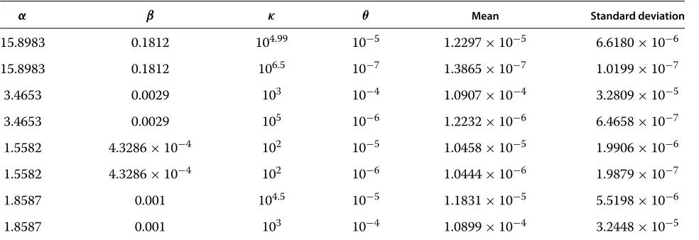
Observe that whenκ = 1, the actual false alarm prob-ability andθ will match exactly due to the detector (7). An analysis of (19) is now undertaken. To begin, the ques-tions of estimator unbiasedness and standard deviation are addressed. It is immediate that ifαandβare unbiased estimators ofαandβ, respectively, then it is unlikely that (19) is also an unbiased estimator of Pfa (also sinceκ >1). Table 1 shows Monte Carlo estimates for the mean and standard deviation of (19), for a selection of clutter param-eter sets and Pfa. The choice for eachκ has been on the basis of the result (14) for examples to be considered in the numerical examples to follow in the next section. Each mean and standard deviation estimate has been generated using a Monte Carlo sample size of 105, together with the Pareto parameter estimation algorithm developed in [27]. The latter uses a property of the Pareto order statistics, together with a linear regression algorithm. Each estimate ofαandβis produced using 1,000 sample points, which is explained in [27] to be sufficient. What is immediate from Table 1 is that the estimator (19) has a bias factor; however, the mean is of the correct order. The standard deviation estimates show that the estimator is efficient.
A mathematical analysis is now included to explore properties of (19) further. It is informative to consider the situation where the actual probability of false alarm is smaller thanθ. Performing some analysis of (19), this will occur whenβκˆ 1/αˆ−βκ1/α>βˆ−β. Hence, define a
func-Observe that the derivative in (20) is positive when
Table 1 Mean and standard deviation ofPfa
α β κ θ Mean Standard deviation
15.8983 0.1812 104.99 10−5 1.2297×10⁻⁵ 6.6180×10⁻⁶
15.8983 0.1812 106.5 10−7 1.3865×10⁻⁷ 1.0199×10⁻⁷
3.4653 0.0029 103 10−4 1.0907×10⁻⁴ 3.2809×10⁻⁵
3.4653 0.0029 105 10−6 1.2232×10⁻⁶ 6.4658×10⁻⁷
1.5582 4.3286×10⁻⁴ 102 10−5 1.0458×10⁻⁵ 1.9906×10⁻⁶
1.5582 4.3286×10⁻⁴ 102 10−6 1.0444×10⁻⁶ 1.9879×10⁻⁷
1.8587 0.001 104.5 10−5 1.1831×10⁻⁵ 5.5198×10⁻⁶
1.8587 0.001 103 10−4 1.0899×10⁻⁴ 3.2448×10⁻⁵
providedα >α. Thus, it is required thatαβ
αβ ≤1. Hence,
assuming these conditions hold, it follows that h is an increasing function fort ≥ 1, and soh(t) ≥ h(1)for all
t ≥1, and the estimated actual probability of false alarm will be smaller thanθ.
An alternative condition can be established by introducing the function
f(t)= t
1+ωt1/α−1 α, (21)
where ω = β/β . Note that f(1) = 1, and so in view of (19), the estimated actual probability of false alarm will be smaller than θ when f is a decreasing function. By applying the quotient differentiation rule, it can be shown that
f (t)= 1−ω+(ω−δ)t
1/α
1+ωt1/α−1 α+1, (22)
whereδ= ααββ. Note that the denominator in (22) is always positive because t ≥ 1. In the case where δ ≥ 1, the derivative is bounded by
f (t)≤ (ω−1)
t1/α−1
1+ωt1/α−1 α+1 <0, (23)
whenω <1, sincet>1.
To summarise these results, the estimated resultant probability of false alarm (19) is smaller than the desired probability of false alarmθ provided the condition
α ˆ α
ˆ β
β ≥1 (24)
holds, together with one of the requirements
(i) α < αˆ (25)
(ii) β < βˆ . (26)
In a practical implementation of the detector (17), using the threshold based upon (13), the hope is that if these condition are valid, we can achieve approximate CFAR control, with at worst a reduction in the desired false alarm rate. Observe that condition (26) justifies the usage of a lower bound on the Pareto scale parameter.
Note that in the case where condition (25) holds, then ifβ > βˆ , it is immediate that (24) is valid. Hence, under-estimating the shape parameter is necessary in practice in order to ensure that the false alarm probability does not increase. This means it will be required to utilise lower bounds on data, coupled with an MLE procedure. The practical implementation of such a scheme, relative to the DSTO Ingara data, will be explored in subsequent research.
As some examples when these conditions are met in practice, suppose we underestimate the Pareto shape parameter with a 10% error, and the Pareto scale parame-ter is overestimated by 10%. By this, it is understood that
α = 0.9α andβ= 1.1β. Then, the conditions (24) and (25) are both met. If both parameters are underestimated by the same percentage error, then (24) will hold, as well as both (25) and (26). If the shape parameter is underesti-mated with an error of 10%, while the scale parameter is underestimated with a 5% error, then all three conditions will also hold.
5 Performance analysis of detectors
WMF (6) are included. Additionally, the NMF (7) is also analysed since it is a special case of the detector (9), which has no requirement for Pareto clutter parameter estimation. In all cases, the detection probability has been estimated using Monte Carlo simulation, with 106runs. The clutter is assumed to have an exponential correlation structure, also known as a Toeplitz form, as in [8] and also [18]. This means we assume(i,j) = ρ|i−j|, where 0 < ρ < 1 and the indicesiandjrange from 1 to the maximum number of looks. In addition, the normalised Doppler frequency has been fixed at 0.5 throughout. A simple Gaussian target model has also been employed in all examples, as in [2,18], which is also known colloqui-ally in the signal processing literature as a Swerling I target model [2].
As remarked previously, clutter parameters will be based upon estimates obtained using MLE on real data sets. The Australian DSTO Ingara data set is a series of pure clutter returns obtained using the Ingara radar during a trial in the Southern Ocean in 2004. The Ingara radar is an airborne X-band, fully polarimet-ric radar, which operated in a circular spotlight mode. Further details concerning this radar can be found in [30], while a thorough analysis of the data is reported in [28]. During the data gathering exercise, the radar surveyed the same ocean patch at different azimuth angles, operating at 10.1 GHz with a 20-μs compressed pulse width, with a range resolution of 0.75 m. The fit-ting of a Pareto intensity model to the Ingara data is described in [14].
The IPIX radar is an experimental X-band search radar belonging to Canada’s McMaster University [31,32], and a clutter collection exercise was undertaken in 1998 as reported in [12]. As detailed in the latter, this radar is capable of dual polarised operations and used a dual fre-quency transmission range of between 8.9 and 9.4 GHz, with a pulse width of 0.06 μs. The range resolution is reported to have been 9 m. The clutter trial was conducted at a fixed location observing Lake Ontario from a height of 20 m so that the radar was stationary. Clutter parameter estimates are reported in [12], which provide a completely different range of Pareto clutter parameters than those obtained from the Ingara radar.
In the analysis to follow, four data sets will be used to present the performance of the detectors under a number of different scenarios. With reference to radar polarisation, throughout, HH will represent horizontal transmit and receive, and VV will be the vertical trans-mit and receive case. No examples of cross polarisation are included due to the fact that clutter parameter esti-mates resulting from this polarisation tend to fall between those obtained from the HH and VV polarisations [18]. Each example is listed by radar, polarisation and clutter parameter estimates. The definition of the inverse gamma
distribution in [12] replacesβ with its reciprocal in (3), which has been taken into account in the IPIX-based examples to follow.
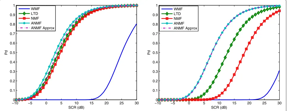
5.1 Ingara, VV,α=15.8983,β=0.1812
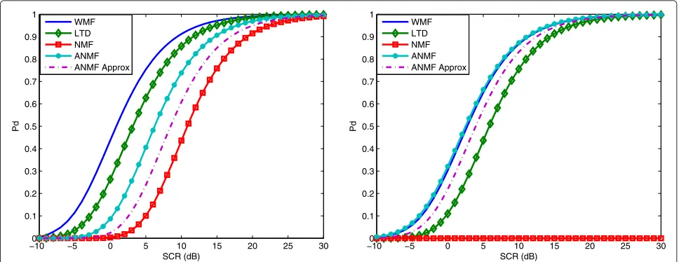
The first example is based upon a typical VV-polarised clutter set obtained from the Ingara data trial. For this particular data set, the Pareto clutter parameters have been estimated to be α = 15.8983 and β = 0.1812. Additionally, this clutter set was obtained at an azimuth angle of 255◦ (upwind direction is approximately 227◦). Figure 1 shows two plots of the performance of the WMF, LTD and NMF when the clutter parameters are assumed to be known. The performance of the detector (9) is also included and is referred to as the alternative NMF (ANMF) in the plots. The left subplot is for the case where the number of looks isN = 5, the Toeplitz fac-tor is ρ = 0.8 and a probability of false alarm is 10−5. With reference to (14), since max{−5,−1.505} = −1.505 and we are examining the VV-polarised case, we select
n = −0.01 so thatκ = 104.99. The plot shows the WMF and ANMF matching very closely, while the LTD has a detection loss relative to these detectors. This is due to the fact that the clutter is approximately Gaussian distributed. The NMF saturates because of the small number of looks. Hence, in this case, we see that the design of the ANMF has improved detection performance in the case of a small number of looks.
The right subplot in Figure 1 is for the same clutter, but whenN = 8,ρ = 0.8 and the false alarm probability is set to 10−7. Hence, since max{−7,−2.408} = −2.408, we selectn= −0.5 to generateκ =106.5. Here, we observe a similar situation to the previous plot, except that the LTD has a larger detection loss relative to the WMF and ANMF. The NMF has again saturated.
Figure 2 examines the performance of the detector (17), relative to the four detectors WMF, LTD, NMF and ANMF, where the latter detectors have full knowledge of clutter parameters. In the figures to follow, detector (17) will be abbreviated to ANMF Approx. In this simu-lation, the left subplot is forN = 20 andρ = 0.5, and the false alarm probability has been set to 10−6. Since max{−6,−6.02} = −6,n= −5 has been selected so that
−100 −5 0 5 10 15 20 25 30 0.1
0.2 0.3 0.4 0.5 0.6 0.7 0.8 0.9 1
SCR (dB)
Pd
WMF LTD NMF ANMF
−100 −5 0 5 10 15 20 25 30
0.1 0.2 0.3 0.4 0.5 0.6 0.7 0.8 0.9 1
SCR (dB)
Pd
WMF LTD NMF ANMF
Figure 1Detector performance in the VV-polarised case, corresponding to clutter simulated from the Ingara radar data trial.Due to the large Pareto shape parameter, the data are roughly Gaussian, resulting in the WMF performing very well. In the left subplot,N=5,ρ=0.8 and probability of false alarm is 10−5. The new detector ANMF matches the WMF almost exactly. Additionally, the ANMF improves on the NMF, which saturates. The right subplot is forN=8,ρ=0.8 and the false alarm probability of 10−7. Here, we can see a difference in the WMF and ANMF. The latter still improves on the NMF.
The right subplot in Figure 2 is for the case where
N = 10,ρ = 0.5 and false alarm probability is 10−7. Noting that max{−7,−3.01} = −3.01,n = −1 has been selected, and consequently, κ = 106. In this example, it is assumed that the shape parameter estimate is overestimated by triple, while the scale param-eter is also overestimated, but by double. The subplot shows the ANMF matching the WMF very closely, while
the estimator (17) has better performance than the LTD. The NMF has completely saturated due to an insuffi-cient number of looks. In this example, the resultant false alarm probability is 2.8255×10⁻⁵, which has been used to set the thresholds for the four other detectors. What is observed here is an increase in the false alarm proba-bility due to severe inaccuracy in the clutter parameter estimates.
−100 −5 0 5 10 15 20 25 30 0.1
0.2 0.3 0.4 0.5 0.6 0.7 0.8 0.9 1
SCR (dB)
Pd
WMF LTD NMF ANMF ANMF Approx
−100 −5 0 5 10 15 20 25 30 0.1
0.2 0.3 0.4 0.5 0.6 0.7 0.8 0.9 1
SCR (dB)
Pd
WMF LTD NMF ANMF ANMF Approx
−100 −5 0 5 10 15 20 25 30 0.1
0.2 0.3 0.4 0.5 0.6 0.7 0.8 0.9 1
SCR (dB)
Pd
WMF LTD NMF ANMF
−100 −5 0 5 10 15 20 25 30 0.1
0.2 0.3 0.4 0.5 0.6 0.7 0.8 0.9 1
SCR (dB)
Pd
WMF LTD NMF ANMF
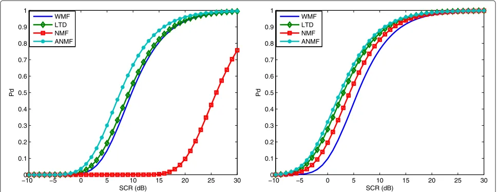
Figure 3Performance analysis in HH-polarised clutter, based upon the Ingara data.The left subplot is forN=20,ρ=0.1 and a false alarm probability of 10−6. This example shows that the ANMF can work very well, and certainly improves on the NMF. The right subplot is for
N=25,ρ=0.1 and false alarm probability of 10−5. In this scenario, we observe the ANMF provides a small gain on the LTD.
5.2 Ingara, HH,α=3.4653,β=0.0029
The second example is for the case of HH-polarised clut-ter, again obtained from the Ingara data trial. In this case, the azimuth angle was 315◦, and the Pareto clutter param-eters areα = 3.4653 and β = 0.0029. Figure 3 shows detector performance when the texture parameters are known. The left subplot is forN = 20,ρ = 0.1 and a false alarm probability of 10−6. Since max{−6,−6.02} =
−6, we have selected n = −1 so that κ = 105. With this choice, it is observed that the ANMF intro-duces a detection gain over the LTD and the WMF. Additionally, the performance of the ANMF far exceeds that of the NMF, which has poorer performance than the WMF.
The right subplot in Figure 3 is forN=25,ρ=0.1 and false alarm probability of 10−5. Since max{−5,−7.525} =
−5, n = −4 has been selected, and hence, κ =
10. Increasing the number of looks has resulted in an improvement on the performance of the NMF, which introduces a detection gain on the WMF. The ANMF has the best performance, with a slight gain on the LTD.
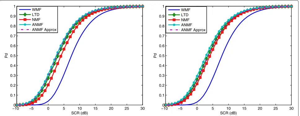
Figure 4 shows some examples of the performance of the detector (17) in horizontally polarised clutter. The left subplot corresponds toN = 30,ρ = 0.5 and a probabil-ity of false alarm of 10−6. Due to max{−6,−9.03} = −6,
n = −5 has been selected so thatκ = 10. It is assumed that both texture parameters have been overestimated by a factor of 5; consequently, the resultant false alarm prob-ability is 3.0169×10⁻⁸, based upon (19). Hence, there is a large reduction in the false alarm probability. All other detectors have had their thresholds set relative to this resultant probability. The subplot shows that the WMF
has very poor performance, as expected in heavy-tailed clutter. The ANMF and LTD have very good perfor-mance, with the ANMF having slightly larger probability of detection. The ANMF approximation (17) has very good performance, despite the inaccuracy with its param-eter estimates. In fact, it is slightly better than the LTD. The NMF’s performance trails that of the LTD. This exam-ple shows that the new CFAR (17) can improve on the NMF considerably.
The right subplot in Figure 4 is for N = 40,ρ =
0.9 and a false alarm probability of 10−7. Due to the fact that max{−7,−12.04} = −7, n = −6 has been selected so thatκ = 10 as previously. Here, it is assumed that the clutter parameter α is overestimated by dou-ble, while there is a 20% error in the estimation of β. The resultant false alarm probability is 3.0169 × 10⁻⁸, which has resulted in an order of magnitude reduction in the desired false alarm rate. The subplot shows similar results to the previous subplot, except that all detectors have closer performance, with the exception of the WMF. The CFAR (17) is matching the performance of the LTD almost exactly in this case.
5.3 IPIX, HH,α=1.5582,β=4.3286×10⁻⁴
−100 −5 0 5 10 15 20 25 30 0.1
0.2 0.3 0.4 0.5 0.6 0.7 0.8 0.9 1
SCR (dB)
Pd
WMF LTD NMF ANMF ANMF Approx
−100 −5 0 5 10 15 20 25 30 0.1
0.2 0.3 0.4 0.5 0.6 0.7 0.8 0.9 1
SCR (dB)
Pd
WMF LTD NMF ANMF ANMF Approx
Figure 4HH-polarisation examples of performance of CFAR (17), relative to Ingara data-based clutter parameter estimates.The left subplot is for the case whereN=30,ρ=0.5 and probability of false alarm is 10−6. Both texture parameters have been overestimated by a factor of 5. Despite this large error, the new CFAR performs very well and certainly improves on the NMF. The right subplot is forN=40,ρ=0.9 and a false alarm probability of 10−7. The clutter parameterαis overestimated by double, while there is a 20% error in the estimation ofβ. As before, we observe that the CFAR (17) has very good performance.
N=30,ρ=0.4 and false alarm probability is 10−6. Since max{−6,−9.03} = −6,n = −4 has been selected and
κ =100. The subplot shows that the WMF has very poor performance. The ANMF improves on the performance of both the LTD and NMF.
The right subplot corresponds to N = 25,ρ =
0.7 and probability of false alarm of 10−5. Due to max{−5,−7.525} = −5,n= −4 has been chosen and so
κ = 10. The results are similar to the previous subplot, except that the performance of the ANMF is much more pronounced. The ANMF is better than the LTD and NMF as before.
Figure 6 shows the performance of the CFAR (17) rel-ative to the other detectors. The left subplot is for N =
30,ρ = 0.4 and a false alarm probability of 10−6. Since max{−6,−9.03} = −6, n = −4 has been selected so
κ = 100. For this simulation, it is assumed that the shape parameterαhas been overestimated by 50%, while the scale parameter is overestimated by 5 times its actual value. This results in an actual false alarm probability of 4.5453×10⁻⁷, which is a reduction in the desired false alarm rate. The subplot shows that the WMF has very poor performance, which is due to the very spiky nature of the clutter. The CFAR (17) has performance bounded above by that of the ANMF and bounded from below by the LTD. Detector NMF has smaller probability of detec-tion than LTD. In this example, the CFAR (17) has very good performance. All detectors have the same probability of false alarm.
The right subplot is for N = 25,ρ = 0.7 and a false alarm probability of 10−7. Since max{−7,−7.525} =
−7,n = −5 has been selected, and hence, κ = 100.
Both clutter parameters are assumed to be underesti-mated by 20%. The resultant false alarm probability can be shown to be 4.4342 × 10⁻⁸, which is a reduction in the design false alarm rate. The subplot shows that the ANMF has the best performance, and the CFAR (17) introduces only a tiny detection loss relative to the ANMF. The LTD has a significant detection loss relative to the ANMF and its approximation. The NMF also has a significant detection loss relative to the ANMF, (17) and the LTD. The WMF has very poor performance in this example.
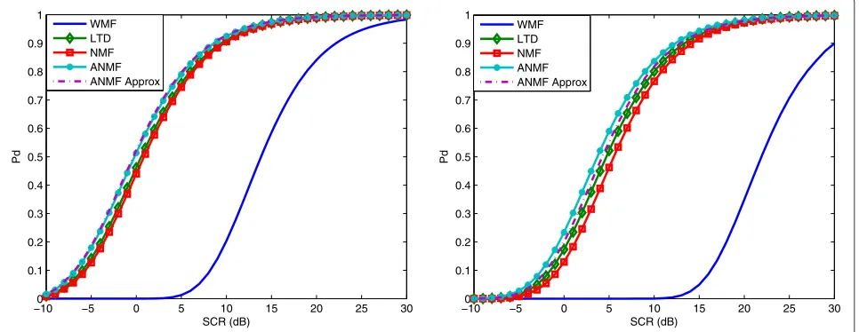
5.4 IPIX, VV,α=1.8587,β=0.001
The final example is for a VV-polarised case based upon the IPIX radar trial. In this scenario, the clut-ter parameclut-ters are α = 1.8587 and β = 0.001. Although this example is for the VV channel, these clut-ter parameclut-ters indicate very heavy-tailed non-Gaussian clutter statistics [33]. Figure 7 shows detector perfor-mance under the assumption of known clutter parame-ters. The left subplot is for N = 30,ρ = 0.6 and a false alarm probability of 10−5. Since max{−5,−9.03} =
−5,n = −3 has been selected, so κ = 100. The sub-plot shows that the WMF has very poor performance. The ANMF has better performance than the LTD and NMF.
The right subplot in Figure 7 is for N = 25,ρ =
0.1 and a false alarm probability of 10−7. Due to max{−7,−7.525} = −7,n = −6 has been chosen, with
−100 −5 0 5 10 15 20 25 30 0.1
0.2 0.3 0.4 0.5 0.6 0.7 0.8 0.9 1
SCR (dB)
Pd
WMF LTD NMF ANMF
−100 −5 0 5 10 15 20 25 30 0.1
0.2 0.3 0.4 0.5 0.6 0.7 0.8 0.9 1
SCR (dB)
Pd
WMF LTD NMF ANMF
Figure 5Detector performance based upon clutter parameter estimates from the IPIX data, HH polarisation.The left subplot is for N=30,ρ=0.4 and a false alarm probability of 10−6. The ANMF has the best performance, while the WMF has the worst, due to the heavy-tailed clutter distribution. The right subplot corresponds toN=25,ρ=0.7 and probability of false alarm of 10−5. Here, the ANMF has a larger gain over the other detectors.
WMF has very poor performance. This is another example showing that the ANMF works very well in spiky clutter.
Figure 8 now examines the performance of the CFAR (17) in this clutter scenario. The left subplot is forN =
40,ρ =0.6 and a false alarm probability of 10−5. In view of the fact that max{−5,−12.04} = −5,n= −4 has been selected so thatκ = 10. It is assumed that the parame-terαis underestimated by 20%, whileβis overestimated by 20%. This results in an actual false alarm probability of 4.2849×10⁻⁶, which is a decrease in the desired false
alarm rate level. The subplot shows that the ANMF and its CFAR approximation (17) have very comparable per-formance, with both detectors performing better than the LTD and NMF. Here, as before, the WMF has the worst performance. All detectors are operating with the same false alarm probability, for consistency.
The right subplot is forN = 30,ρ = 0.1 and a false alarm probability of 10−7. Since max{−7,−9.03} = −7,
n= −6 has been selected, yieldingκ=10. For this exam-ple, the Pareto shape parameter is overestimated by 80%,
−100 −5 0 5 10 15 20 25 30 0.1
0.2 0.3 0.4 0.5 0.6 0.7 0.8 0.9 1
SCR (dB)
Pd
WMF LTD NMF ANMF ANMF Approx
−100 −5 0 5 10 15 20 25 30 0.1
0.2 0.3 0.4 0.5 0.6 0.7 0.8 0.9 1
SCR (dB)
Pd
WMF LTD NMF ANMF ANMF Approx
−100 −5 0 5 10 15 20 25 30 0.1
0.2 0.3 0.4 0.5 0.6 0.7 0.8 0.9 1
SCR (dB)
Pd
WMF LTD NMF ANMF
−100 −5 0 5 10 15 20 25 30 0.1
0.2 0.3 0.4 0.5 0.6 0.7 0.8 0.9 1
SCR (dB)
Pd
WMF LTD NMF ANMF
Figure 7Detector performance with clutter parameter estimates based upon the IPIX radar trial, with VV polarisation.The left subplot is forN=30,ρ=0.6 and a false alarm probability of 10−5. The ANMF has a gain over all other detectors. The right subplot is forN=25,ρ=0.1 and a false alarm probability of 10−7. Again, the ANMF has very good performance. Due to the heavy-tailed nature of the clutter, the WMF has very poor performance.
while the scale parameter is overestimated by 20%. This results in an actual false alarm probability of 2.3328 × 10⁻⁷, which is larger than the desired false alarm rate. The plot shows similar results to the previous subplot, except that it is easier to discern the differences in detector per-formance. Again, the ANMF has the best performance, and the CFAR (17) has very good performance.
6 Conclusions
This paper introduced a modification of the NMF detec-tor, referred to as the ANMF and given by (9), which was
shown to work very well in practice. By using a parameter
κ, which is a function of the design false alarm probability and the number of looks, and whose value is then deter-mined by an application of (14), one can avoid the detector saturation issues inherent in the NMF. This new detector was shown to outperform the LTD and WMF in a large number of cases, when clutter parameters are known. In particular, this tended to occur for the case where the number of looks was large (N >> 30), and the clut-ter is very spiky. In addition to this, by then introducing approximations to the clutter parameters, an approximate
−100 −5 0 5 10 15 20 25 30 0.1
0.2 0.3 0.4 0.5 0.6 0.7 0.8 0.9 1
SCR (dB)
Pd
WMF LTD NMF ANMF ANMF Approx
−100 −5 0 5 10 15 20 25 30 0.1
0.2 0.3 0.4 0.5 0.6 0.7 0.8 0.9 1
SCR (dB)
Pd
WMF LTD NMF ANMF ANMF Approx
Figure 8Analysis of the CFAR detector (17) in the same clutter environment as for Figure 7.The left subplot is for the case where
CFAR version of this detector was analysed. It was shown to perform very well in practice, depending on the error in the approximation of the clutter parameters. The error in clutter parameter estimation resulted in a change in the desired false alarm probability. Some conditions were established to ascertain when there was not an increase in the false alarm rate. Provided that the clutter parameter errors were small, there were only small variations in the false alarm rate, as expected. Despite this, the CFAR (17) was shown to have very good performance in practice.
In further research, the detector (17) will be applied to real data to assess its performance in practice. This will be coupled together with real-time parameter estimation based upon the work of [27].
Abbreviations
ANMF: Alternative normalised matched filter; CFAR: Constant false alarm rate; DSTO: Defence Science and Technology Organisation; GLRT: Generalised likelihood ratio test; HH: Horizontal transmit and receive; LTD: Linear threshold detector; MLE: Maximum likelihood estimation; NMF: Normalised matched filter; Pd: Probability of detection; Pfa: Probability of false alarm; SCR: Signal-to-clutter ratio; SIRP: Spherically invariant random process; VV: Vertical transmit and receive; WMF: Whitening matched filter.
Authors’ contributions
The author declares that there are no competing interests.
Acknowledgements
The author would like to express thanks to an anonymous reviewer whose comments significantly improved the content and results of this paper.
Received: 8 January 2013 Accepted: 2 May 2013 Published: 15 May 2013
References
1. KJ Sangston, F Gini, inIEEE Radar Conference. MS Greco, New results on coherent radar target detection in heavy-tailed compound Gaussian clutter, Washington, DC, 2010), pp. 779–784. 10–14 May
2. KJ Sangston, F Gini, MS Greco, Coherent radar target detection in heavy-tailed compound Gaussian clutter. IEEE Trans. Aerosp. Electron. Syst.48, 64–77 (2012)
3. E Conte, M Longo, Characterisation of radar clutter as a spherically invariant random process. IEE Proc, Pt. F: Commun. Radar Signal Process. 134, 191–197 (1987)
4. M Rangaswamy, D Weiner, A Ozturk, Non-Gaussian random vector identification using spherically invariant random processes. IEEE Trans. Aerosp. Elec. Syst.29, 111–123 (1993)
5. KJ Sangston, K Gerlach, Coherent detection of radar targets in a non-Gaussian background. IEEE Trans. Aerosp. Electron. Syst.3, 330–340 (1994)
6. F Gini, Suboptimal coherent radar detection in a mixture of K-distributed and Gaussian clutter. IEE Proceed. Part F: Radar, Sonar, Navig.144, 39–48 (1997)
7. F Gini, MV Greco, A Farina, P Lombardo, Optimum and mismatched detection against K-distributed plus Gaussian clutter. IEEE Trans. Aerosp. Electron. Syst.34, 861–876 (1998)
8. F Gini, MV Greco, Suboptimal approach to adaptive coherent radar detection in compound Gaussian clutter. IEEE Trans. Aerosp. Electron. Syst.35, 1095–1104 (1999)
9. E Conte, M Lops, G Ricci, Asymptotically optimum radar detection in compound Gaussian clutter. IEEE Trans. Aerosp. Elec. Sys.31, 617–625 (1995)
10. Y Dong, Optimal coherent radar detection in a K-distributed clutter environment. IET Radar, Sonar Navig.6, 238–292 (2012)
11. GV Weinberg, inDigital Communication, ed. by C Palanisamy. Coherent multilook radar detection for targets in KK-distributed clutter (Intech, Croatia, 2012)
12. A Balleri, A Nehorai, J Wang, Maximum likelihood estimation for compound-Gaussian clutter with inverse-gamma texture. IEEE Trans. Aerosp. Electron. Syst.43, 775–780 (2007)
13. M Farshchian, FL Posner, inIEEE Radar Conference. The Pareto distribution for low grazing angle and high resolution X-band sea clutter,
Washington, DC, 2010), pp. 789–793. 10–14 May
14. GV Weinberg, Assessing the Pareto fit to high resolution high grazing angle sea clutter. IET Electron. Lett.47, 516–517 (2011)
15. X Shang, H Song, Radar detection based on compound-Gaussian model with inverse gamma texture. IET Radar, Sonar, Navig.5, 315–321 (2011) 16. GV Weinberg, Coherent multilook radar detection for targets in Pareto
distributed clutter. IET Electron. Lett.47, 822–824 (2011)
17. P Stinco, M Greco, F Gini, Adaptive detection in compound-Gaussian clutter with inverse gamma texture. IEEE Int. Conf. Radar.1, 434–437 (2011)
18. GV Weinberg, Assessing detector performance, with application to Pareto coherent multilook radar detection. IET Radar, Sonar, Navig.7(2013) (in press)
19. GP Beaumont,Intermediate Mathematical Statistics. (Chapman and Hall, London, 1980)
20. G Minkler, J Minkler,CFAR: The Principles of Automatic Radar Detection in Clutter. (Magellan, Baltimore, 1990)
21. J Guan, YN Peng, Y He, Proof of CFAR by the use of the invariant test. IEEE Trans. Aerosp. Elec. Sys.36, 336–339 (2000)
22. KJ Sangston, F Gini, MV Greco, A Farina, Structures for radar detection in compound Gaussian clutter. IEEE Trans. Aerosp. Elec. Sys.35, 445–458 (1999)
23. R Ravid, N Levanon, Maximum-likelihood CFAR for Weibull background. IEE Proceed. F.139, 256–264 (1992)
24. V Anasstassopoulos, GA Lampropoulos, Optimal CFAR detection in Weibull clutter. IEEE Trans. Aerosp. Elec. Sys.31, 52–64 (1995) 25. P Billingsley,Probability and Measure (2nd Ed). (Wiley, New York, 1986) 26. RG Kuller,Topics in Modern Analysis. (Prentice-Hall, Englewood Cliffs, 1969) 27. GV Weinberg, Estimation of Pareto clutter parameters using order
statistics and linear regression. IET Electron. Lett (2013). (in press) 28. Y Dong, Distribution of X-band high resolution and high grazing angle
sea clutter (DSTO Technical Report RR-0316,2006) (2013). http://www. dtic.mil/cgi-bin/GetTRDoc?AD=ADA462947, Accessed 12 May 29. N Stacy, D Crisp, A Goh, D Badger, M Preiss, Polarimetric analysis of fine
resolution X-band sea clutter data. Proceed. Int. Geoscience Remote Sensing Symp.4, 2787–2790 (2005)
30. NJS Stacy, MP Burgess, Ingara: the Australian airborne imaging radar system. Proceed. Int. Geoscience Remote Sensing Symp.4, 2240–2242 (1994)
31. TJ Nohara, S Haykin, Canadian east coast radar trials and the K-distribution. IEE Proc. F.138, 80–88 (1991)
32. A Farina, F Gini, MV Greco, L Verrazzani, High resolution sea clutter data: statistical analysis of recorded live data. IEE Proc. -Radar, Sonar, Navig. 144, 121–130 (1997)
33. GV Weinberg, Validity of whitening matched filter approximation to the Pareto coherent detector. IET Sig. Proc.6, 546–550 (2012)
doi:10.1186/1687-6180-2013-105