Simulation of the acoustic wave propagation using a meshless method

Simulation of the acoustic wave propagation using a meshless method

J.Bajko1a,P.Niedoba1, L. ˇCerm´ak1, and M.J´ıcha1

1_{Energy Institute, Department of Thermodynamics and Environmental Engineering, Brno University of}

Tech-nology, Technick´a 2896/2, 616 69 Brno, Czech Republic

Abstract. This paper presents numerical simulations of the acoustic wave propagation phenomenon modelled via Linearized Euler equations. A meshless method based on collocation of the strong form of the equation system is adopted. Moreover, the Weighted least squares method is used for local approximation of derivatives as well as stabilization technique in a form of spatial filtering. The accuracy and robustness of the method is examined on several benchmark problems.

1 Introduction

Numerical study of sound generation and propaga-tion phenomenon plays a major role in Computapropaga-tional Aeroacoustics (CAA), especially in predictions of sound generated by turbulent flows and its environmental consequences. This paper is aiming to contribute to the development of suitable methods for sound prop-agation simulations governed by the Linearized Euler equations (LEE), cf. [1, 2].

Various numerical mesh-based methods, cf. [3, 4], have been investigated in this context, but there is also growing interest in meshless methods, cf. [5–11], due to their potential advantages. Depending on applica-tions, these methods can be superior in accuracy, sta-bility, robustness and can deal with complex geome-tries, multiphase flow, problems with free boundaries and moving objects. In this paper, the development of a meshless method adjusted for linear systems is outlined.

Firstly, LEE as a linear hyperbolic system is in-troduced, followed by the Weighted Least SQuares (WLSQ) method which is employed in two ways - for local interpolation of acoustic variables and for spatial filtering, cf. [12, 13]. The WLSQ filtration technique serves primarily for the stabilization of the numerical scheme and can be utilized under the assumption that the governing equations are linear and the solution is smooth enough.

Finally, abilities of the method are demonstrated on various benchmark problems for the acoustic wave propagation, cf. [14–16]. The method is tested on un-structured point distributions and several types of bound-ary conditions (BC) are implemented, namely the non-reflecting BC realized by the Perfectly Matched Layer (PML), cf. [17–19].

a _{Present address: [email protected]}

2 Linearized Euler equations

The hyperbolic non-homogeneous LEE represent one of the suitable models for the acoustic wave propa-gation phenomenon. We consider the 2D matrix form (x= (x, y)∈Ω, t >0) written as

∂w

∂t +A1(w0) ∂w

∂x +A2(w0) ∂w

∂y =S, (1)

where

w_{(x, t) =}

⎛ ⎜ ⎜ ⎝

ρ(x, t) u(x, t) v(x, t) p(x, t)

⎞ ⎟ ⎟

⎠, w0(x) = ⎛ ⎜ ⎜ ⎝

ρ0(x) u0(x) v0(x) p0(x)

⎞ ⎟ ⎟ ⎠, (2)

Vector function w(x, t) denotes the time dependent acoustic variables (density, velocity components and pressure) and w₀(x) steady mean flow variables cor-responding to the underlying flow field.

Jacobian matrices of the system (1) are given as

A1= ⎛ ⎜ ⎜ ⎝

u0 ρ0 0 0 0 u0 0 _ρ01 0 0 u0 0 0 γp0 0 u0

⎞ ⎟ ⎟ ⎠,A2=

⎛ ⎜ ⎜ ⎝

v0 0 ρ0 0 0 v0 0 0 0 0 v0 ρ01 0 0 γp0 v0

⎞ ⎟ ⎟ ⎠, (3)

where γ = 1.4 is the ratio of specific heats and S= S(x, t) represents the acoustic source term, cf. [1, 2].

The initial–value boundary problem for LEE then consists of the equation system (1) with the initial and boundary condition

(IC) w(x,0) =w_in (x), x∈Ω, (4)

3 Meshless method with WLSQ filtering

In the context of meshless methods we distiguish be-tween the global cloud ˆΩdefined as a set ofnpoints discretizing a domain of interest Ω and local clouds

ˆ

Ωi, i= 1, . . . , nthat are calculated in the pre-processing step of the simulation. Ani-th local cloud usually con-sists of a set ofnineighbours chosen by a certain rule. Practically, efficient algorithms for nearest neighbor search such as the k-d tree are used. Therefore, the number of pointsni is controlled by the radius of an open ball or it can be prescribed manually.

3.1 Weighted Least Squares Method

For every local cloud ˆΩi we wish to find a local ap-proximation ˆw:Ωi→Rin the form

ˆ w(x) =

m

l=1

αlpl(x) =pT(x)α (6)

where

pT_{(x) = (p}

1(x), p2(x), . . . , pm(x)) (7)

and

α= (α1, α2, . . . , αm)T ∈Rm. (8) Functionspl:Rd→R, l= 1, . . . , m, form a basisBof an approximation spaceF = span(B). The complete (multivariate) polynomial basis of degreeν, cf. [5, 10] is adopted in this work. Ford= 2 andν= 3, the basis

B= 1, x, y, x2, xy, y2, x3, x2y, xy2, y3. (9)

3.2 WLSQ approximation

It is well known that WLSQ method finds the coeffi-cients α in (6) by minimizing the objective function J(α) with weights

J(α) = (Pα−w)TΦ(Pα−w), (10)

wherePdenotes the moment matrix of type (ni×m), Φ the diagonal weight matrix of orderni and w the vector of given function values. The weighting function φ:Rd→Rprescribes the contribution of every point to J(α) in the local cloud according the distance to the star pointxi

1, cf. [10].

Solution to the system ofnormal equations

PT_ΦPα=PT_{Φw. (11)}

then yields

α=PTΦP−1PTΦw (12)

assumming the invertibility of the above mentioned matrix. We suppose that the number of points ni in

ˆ

Ωi is greater than the number of basis functions m, i.e.ni> mholds.

3.3 WLSQ interpolation

By adding theinterpolation constraint

ˆ

w(xi₁) =w1, (13)

to the Normal equations (11), the value w1 is repro-duced at the star point x_i exactly. This modification can be gently implemented and allows to use the WLSQ method for multiple purposes, namely the spatial dis-cretization of the governing equations (interpolation) as well as numerical filtering (approximation).

3.4 Spatial discretization of LEE

In order to obtain the semi–discrete form of governing equations (1), the collocation method is adopted, i.e. the expression

∂wˆ

∂t +A1 ∂wˆ

∂x +A2 ∂wˆ

∂y −S

x=xi

= 0 (14)

has to be satisfied. Acoustic variables ˆwi are locally approximated using WLSQ method with interpolation condition described in section (3.1).

The collocation then leads to a system of ordinary differential equations (ODE) in form

dw_i(t)

dt =RHSi(t) +S(xi, t) (15)

where RHSi(t) contains contributions to the right-hand side from all neighbours of the star pointx_i, cf. [7, 10, 11]. The interpolation condition in the WLSQ approach allows to simplify the left side of the equa-tion system (15) avoiding the necessity to solve the system ofnlinear equations. Therefore, using WLSQ with interpolation condition greatly reduces the com-putation costs and improves stability, cf. [10, 11]. The system of ODE (15) is then solved with high order low-dissipation and low-dispersion runge-kutta scheme op-timized for wave propagation problems, cf. [20].

3.5 Numerical filtering

Thei-th local cloud ˆΩi is utilized for filtering after every time step in a way that wi(t) ≈ w(xi, t) is replaced by the filtered value

wi(t) =pT(xi)α (16)

at the star pointxi.

3.6 Boundary conditions

Firstly, solid–wall slip BC is prescribed at points where the acoustic waves should be reflected. The acoustic velocity vector v = (u, v) at the boundary point x∈Γ is forced to stay orthogonal to the normal vec-torn= (nx, ny), i.e.

v_{·n= 0. (17)}

Secondly, non–reflecting BC is prescribed at do-main boundaries, where waves should leave the com-putational domain without any reflection. It can be achieved artificially by designing a layer of points around the domain of interest that will affect the solution in such a way that the major spectrum of incoming waves will dissipate. The PML is implemented in our numer-ical experiments, cf. [17–19].

4 Numerical experiments

4.1 2D Wall-reflected acoustic pulse problem

This benchmark problem is designed to verify the im-plementation of the wall boundary condition and the accuracy and stability of a numerical method when a reflection of an acoustic wave from the solid wall oc-cur. Let us consider a 2D domainΩ= (−100,100)×

0,150) that is depicted in Fig. 1 together with an initial pulse located at (xp, yp) = (0,25). The wall boundary condition is prescribed at line y = 0. We suppose the underlying medium at rest, which implies that the mean flow velocity equals zero and therefore the Mach numberM = 0 and forw₀ it holds

ρ0= 1, u0=v0= 0, p0= ρ0 γ =

5

7. (18)

The Initial-value boundary problem consists of the equation system (1) with the source termS=0, above mentioned boundary conditions and initialized by the initial conditionw(x, y,0) given as follows

w

in(x, y) =εexp(−κr2p) (1,0,0,1)T, (19)

where the radius rp =

(x−xp)2+ (y−yp)2 and κ = (ln 2)/b2. The amplitude and the half–width of the acoustic initial pulse are determined byε= 1 and b= 5, respectively.

x y

200 150

25

Fig. 1. Rectangular domain Ω, wall (solid line) and ex-ternal boundary (dashed line).

4.1.1 Numerical solution

Results of the acoustic wave simulation in terms of the acoustic pressure contours are plotted ase a series of Fig. (2–5) at particular times T = 10,25,50,75. The time integration was performed with time step dt= 0.025 that corresponds to the unstructured point distribution withn= 36006 number of points.

Fig. 2.Ac. pressurep(x, y, T) contours at timeT = 10.

The comparison of the acoustic pressurep(x, y, T) along the line x = 0 and analytical solution at time T = 75 is shown in Fig. 6.

4.2 2D Convected acoustic monopole

Fig. 3. Ac. pressurep(x, y, T) contours at timeT = 25.

Fig. 4. Ac. pressurep(x, y, T) contours at timeT = 50.

Fig. 5. Ac. pressurep(x, y, T) contours at timeT = 75.

Fig. 6. Ac. pressurep(x, y, T) along the linex= 0.

x y

Ωe

M0= 0.5

100 100

50 50

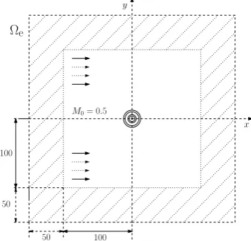
Fig. 7. Square domainΩ, PML layerΩ_e (shaded region) and external boundary (dashed line).

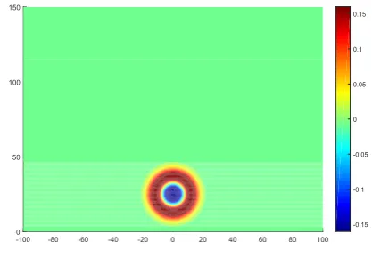
We will consider subsonic underlying mean flow in x-direction with Mach number M0 = 0.5 as well as supersonic flow with M0 = 1.5. In this example, the acoustic source term on the right-hand side of the sys-tem (1) is the periodic perturbation of acoustic density and pressure at the origin xs=ys= 0 which is given as

S(x, t) =e−α((x−xs)2+(y−ys)2) sin(ωt)(1,0,0,1)T (20) where α = ln(2)/2, amplitude ε = 0.5 and angular frequencyω= 2π/30.

Fig. 8. Subsonic flow - acoustic pressure p(x, y, T) con-tours at timeT= 270.

Fig. 9. Supersonic flow - detail of the acoustic pressure

p_{(x, y, T) contours at timeT = 270.}

4.3 2D Acoustic monopole in a sheared mean flow

Prescribing the velocity components in (18) in form

u0(x, y) =umaxtanh(2y/δ), v0= 0 (21)

we get the non-constant underlying flow known as sheared mean flow, cf. [1, 15]. In this example, the peak velocity is taken as umax = 0.5 and the shear layer thickness δ = 150. The convection velocity profile is depicted in Fig. 10.

Instantaneous acoustic pressure contours at time T = 270 are plotted in Fig. 11.

5 Discussion

Linearity of governing equations (LEE) and therefore the absense of shock waves and strong disturbances

Fig. 10.Velocity profileu0(x, y)

Fig. 11.Acoustic pressurep(x, y, T) at timeT = 270.

in the solution allowed to develop a new stabilization technique in a meshless framework. Instead of the up-wind approximation of derivatives widely used, e.g. in Finite volume methods, the stability of the meshless method was achieved by the WLSQ filtering of the numerical solution after each time step.

The method was tested on acoustic benchmark problems, such as the 2D wall bounded acoustic pulse problem and the acoustic monopole in a free stream and sheared mean flow. In order to suppress waves leaving the domain, the non-reflecting boundary con-dition in form of the PML was sucessfully utilized, cf. Fig. 8. To conclude, the method proved its ability to solve the wave propagation problems governed by LEE in various settings and is prepared for further applications.

Acknowledgement

References

1. Ch. Bailly, D. Juv´e, AIAA38(2000).

2. W.D. Roeck,Hybrid Methodologies for the compu-tational Aeroacoustic Analysis of Confined, Subsonic Flows, Katholieke Universiteit Leuven (2007). 3. Ch.K.W. Tam, J.C. Webb, J. Comput. Phys.107

262–281 (1993).

4. X. Nogueira, S. Khelladi, I. Colominas, L. Cueto-Felgueroso, J. Par´ıs, H. G´omez, Arch. Comput. Meth. Eng.18315–340 (2011).

5. G.R. Liu, Y.T. Gu, An Introduction to Meshfree Methods and Their Programming (2005).

6. G.E. Fasshauer, Meshfree Approximation Methods with Matlab,6, ISBN: 978-981-270-634-8, (2007). 7. J. Bajko, L. ˇCerm´ak, M. J´ıcha, Comput. Meth.

Appl. Mech. Eng. 280157–175 (2014). 8. A.J. Katz, A. Jameson, AIAA6992008.

9. A.J. Katz: Meshless methods for computational fluid dynamics, Stanford University (2009).

10. E. Ortega, E. O˜nate, S. Idelsohn, Int. J. Numer. Meth. Fluids 60937–971 (2009).

11. R. L¨ohner, C. Sacco, E. O˜nate, S. Idelsohn, Int. J. Numer. Meth. Eng.53, 1765–1779 (2002). 12. A. Savitzky, M. J. E. Golay, Anal. Chem. 36(8)

1627–1639 (1964).

13. P.A. Gorry, Anal. Chem.62(6)570–573 (1990). 14. Ch. K. W. Tam,Benchmark Problems and

Solu-tions, 1-13 (1995).

15. R. Ewert, W. Schr¨oder, J. Comput. Phys.188(2) 365–398 (2003).

16. K. Li, Q.B. Huang, J.L. Wanga, L.G. Lin, Eng. Anal. Boundary Elem.35 47–55 (2011).

17. T. Colonius, Annu. Rev. Fluid Mech.36 315–45 (2004).

18. F. Q. Hu, J. Comput. Phys.175455–480 (2001). 19. F. Q. Hu, J. Comput. Phys.208, 469–492 (2005). 20. F.Q. Hu, M.Y. Hussainy, J.L. Manthey, J.