Classifying music perception and imagination using EEG

Western University Western University

Scholarship@Western

Scholarship@Western

Electronic Thesis and Dissertation Repository

5-12-2016 12:00 AM

Classifying music perception and imagination using EEG

Classifying music perception and imagination using EEG

Avital Sternin

The University of Western Ontario

Supervisor Dr. Jessica Grahn

The University of Western Ontario Joint Supervisor Dr. Adrian Owen

The University of Western Ontario Graduate Program in Psychology

A thesis submitted in partial fulfillment of the requirements for the degree in Master of Science © Avital Sternin 2016

Follow this and additional works at: https://ir.lib.uwo.ca/etd

Part of the Cognitive Neuroscience Commons

Recommended Citation Recommended Citation

Sternin, Avital, "Classifying music perception and imagination using EEG" (2016). Electronic Thesis and Dissertation Repository. 3769.

https://ir.lib.uwo.ca/etd/3769

This Dissertation/Thesis is brought to you for free and open access by Scholarship@Western. It has been accepted for inclusion in Electronic Thesis and Dissertation Repository by an authorized administrator of

Abstract

This study explored whether we could accurately classify perceived and imagined musical

stimuli from EEG data. Successful EEG-based classification of what an individual is

imag-ining could pave the way for novel communication techniques, such as brain-computer

inter-faces. We recorded EEG with a 64-channel BioSemi system while participants heard or

imag-ined different musical stimuli. Using principal components analysis, we identified components common to both the perception and imagination conditions however, the time courses of the

components did not allow for stimuli classification. We then applied deep learning techniques

using a convolutional neural network. This technique enabled us to classify perception of music

with a statistically significant accuracy of 28.7%, but we were unable to classify imagination

of music (accuracy=7.41%). Future studies should aim to determine which characteristics of music are driving perception classification rates, and to capitalize on these characteristics to

raise imagination classification rates.

Keywords:music perception, music imagination, classification, electroencephalography (EEG), machine learning, deep learning, neural network, brain-computer interface (BCI)

Acknowledgements

Thank you to my supervisors, Dr. Jessica Grahn and Dr. Adrian Owen, for guiding me through this project. Without their support, encouragement, and tireless editing, this document would not be in your hands today.

Thank you to Dr. Sebastian Stober for his machine learning expertise and for pushing me to explore new and difficult topics.

Thank you to the members of the Owen and Grahn Labs for their invaluable suggestions, feedback, and assistance at each stage of this experiment.

Thank you to those who called the first floor of the Brain and Mind Institute home. They helped me grapple with difficult concepts while being the kindest friends one could ask for.

Thank you to my family for supporting me in this endeavour, especially to my father for teaching me how to be a scientist.

Contents

Abstract i

Acknowledgements ii

List of Tables v

List of Figures vi

List of Appendices viii

1 Introduction 1

2 Methods 7

2.1 Participants . . . 7

2.2 Stimuli . . . 7

2.3 Equipment and Procedure . . . 8

2.3.1 Behavioural Testing . . . 8

2.3.2 EEG recording . . . 10

2.4 Preprocessing . . . 12

3 ERP Analysis 14 4 Neural Network 18 4.1 Layer 1: Similarity Constraint Encoding . . . 19

4.2 Layer 2: Temporal Filter & Layer 3: Templates . . . 21

4.3 Full model explanation . . . 22

4.4 Results . . . 23

4.5 Discussion . . . 27

5 Behavioural Experiment 29 5.1 Participants . . . 29

5.2 Procedure . . . 29

5.3 Results . . . 30

6 Discussion 33

References 39

A Ethics Approval Form 42

B Questionnaire 43

C Neural Net Classification Using PCA Derived Filters 46

Curriculum Vitae 49

List of Tables

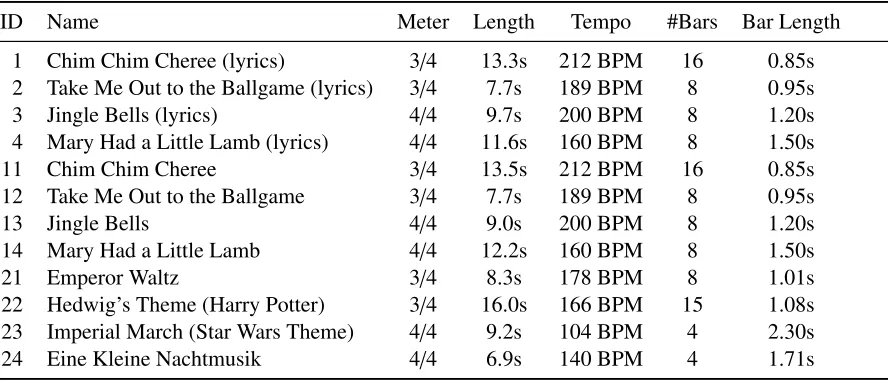
2.1 Tempo, meter and length of the stimuli used in the experiment. . . 9

List of Figures

2.1 Setup for the EEG experiment. The presentation and recording systems were placed outside to reduce the impact of electrical line noise that could be picked up by the EEG amplifier. . . 10 2.2 Illustration of the design for the EEG portion of the study. . . 11

3.1 Topographic visualization of the top 4 principal components with percentage of the explained signal variance. Channel positions in the 64-channel EEG layout are shown as dots. Colors are interpolated based on the channel weights. The PCA was computed onA: the grand average event-related potentials (ERPs) of all perception trials;B: the grand average ERPs of all cued imagination trials; C: the concatenated perception trials;D: the concatenated cued imagination trials. 15 3.2 The time course of component three during perception (blue) and imagination

(red) of Eine Kleine Nachtmusic. The correlation between the two time courses isr(190)=0.40 (p<0.001). . . 16 3.3 The time course of component three during perception (blue) and imagination

(red) of The Emperor Waltz. The correlation between the two time courses is

r(190)=0.30 (p<0.001). . . 16 3.4 The time course of component three during perception (blue) of the Star Wars

theme and imagination (red) of Jingle Bells (no lyrics). The correlation be-tween the two time courses isr(190)=0.52 (p<0.001). . . 17 4.1 Visualization of our neural network, which processes raw EEG at a sampling

rate of 512 Hz. Layer 1 was pre-trained using similarity-constraint encoding and is a spatial representation of EEG electrode weights. Layer 2 is a 37 sample long temporal filter. Layer 3 shows the compressed representations of the raw EEG data. The numbers are the ID numbers of the stimuli found in Table 2.1. The colours are an indication of the weighting decided on by the model. We can interpret the intense red and blue colours as being more important for stimulus classification than the white areas. . . 21 4.2 12-class confusion matrix for perception data. The numbers along the axes

cor-respond to the ID numbers of the stimuli found in Table 2.1. Intensity indicates the number of times a true label was classified as a predicted label with darker colours indicating more classifications. . . 23

4.3 Binary confusion matrices for perception data. The inset shows the p-values determined by using the cumulative binomial distribution to estimate the like-lihood of observing the respective binary classification rate by chance. The significance threshold was bonferroni corrected toalpha=0.05/66=7.5e-04 . 24 4.4 12-class confusion matrix for imagination data. The numbers along the axes

correspond to the ID numbers of the stimuli found in Table 2.1. Intensity indi-cates the number of times a true label was classified as a predicted label with darker colours indicating more classifications. . . 25 4.5 Binary confusion matrices for imagination data. The inset shows the p-values

determined by using the cumulative binomial distribution to estimate the like-lihood of observing the respective binary classification rate by chance. The significance threshold was bonferroni corrected toalpha=0.05/66=7.5e-04 . 26 5.1 Average time it takes for participants to recognize these stimuli (red).

Indi-vidual data is shown in black and song length is shown in blue. The magenta bars indicate the highlighted time periods from layer three in the neural net (Figure 4.2). . . 31 5.2 Similarity ratings (from 0-100) of binary comparisons of all stimuli. . . 32 C.1 Principal component analysis (PCA) done on all perception training trials (432

trials) . . . 46 C.2 Classification results when layer 1 of the neural net is replaced with the first

component from Figure C.1 . . . 46 C.3 Classification results when layer 1 of the neural net is replaced with the second

component from Figure C.1 . . . 47 C.4 Classification results when layer 1 of the neural net is replaced with the third

component from Figure C.1 . . . 47 C.5 Classification results when layer 1 of the neural net is replaced with the fourth

component from Figure C.1 . . . 48

List of Appendices

Appendix A Ethics Approval Form . . . 42 Appendix B Questionnaire . . . 43 Appendix C Neural Net Classification Using PCA Derived Filters . . . 46

Chapter 1

Introduction

The vast majority of people imagine music. Imagining music can be defined as a

deliber-ate internal recreation of the perceptual experience of listening to music (Schaefer, Farquhar,

Blokland, Sadakata, & Desain, 2011). Individuals can imagine themselves producing music,

imagine listening to others produce music, or simply “hear” the music in their heads.

Mu-sic imagination is used by muMu-sicians to memorize muMu-sic, and anyone who has ever had an

“ear-worm” – a tune stuck in their head – has experienced imagining music. Because of its

simplicity, no training is required to imagine a song, and researchers have therefore been

inves-tigating the utility of music imagery for brain-computer interfaces (BCIs). A BCI is a system

that allows an external device to be controlled or modified using brain activity. Music imagery

appears to be a very promising means for driving BCIs that use electroencephalography (EEG)

– a popular non-invasive neuroimaging technique that relies on electrodes placed on the scalp

to measure the electrical activity of the brain. For instance, Schaefer et al. (2011) argue that

“music is especially suitable to use here as (externally or internally generated) stimulus

ma-terial, since it unfolds over time, and EEG is especially precise in measuring the timing of a

response.” For patients that have difficulties communicating behaviourally (e.g., patients with locked-in syndrome), BCIs are a promising communication tool. BCIs that currently exist are

generally binary systems that allow the user to choose between two options to answer yes/no questions (Monti et al., 2010). A system with a larger number of options would allow for a

2 Chapter1. Introduction

more complete and efficient communication experience. Using music as the basis for a BCI is a promising way to build such a system because of the large number of musical pieces that

exist. Ideally, a music-based BCI would allow the user to imagine a piece of music to

con-vey a particular thought. However, the translation from music imagination will require careful

processing of the EEG data.

EEG data contain a variety of signals (elicited by external stimuli like sounds, lights etc.)

that can be exploited by a BCI. For a BCI to be successful, it must be able to distinguish

be-tween different induced brain states. Perceived rhythmic sequences have been shown to alter EEG signals resulting in unique brain states. It has been shown that oscillatory neural activity

in the gamma frequency band (20-60 Hz) is sensitive to accented tones in a rhythmic sequence

(Snyder & Large, 2005). Oscillations in the beta band (20-30 Hz) entrain to rhythmic sequences

(Cirelli et al., 2014; Merchant, Grahn, Trainor, Rohrmeier, & Fitch, 2015) and increase in

an-ticipation of strong tones in a non-isochronous, rhythmic sequence (Iversen, Repp, & Patel,

2009; Fujioka, Trainor, Large, & Ross, 2009, 2012). The magnitude of steady state evoked

potentials (SSEPs), which reflect neural oscillations entrained to the stimulus, increases in

fre-quencies related to the metrical structure of the rhythm when subjects hear rhythmic sequences.

In addition, perturbations of the rhythmic pattern lead to distinguishable ERPs (Geiser, Ziegler,

Jancke, & Meyer, 2009; Vlek, Schaefer, Gielen, Farquhar, & Desain, 2011). It is also

possi-ble to detect imagined auditory accents imposed over a steady metronome click from EEG

(Nozaradan, Peretz, Missal, & Mouraux, 2011). Finally, EEG signals have been used to

3

alters EEG patterns in systematic ways that may be exploited by a BCI. Because rhythm is an

inherent part of music, we expect music to have a similar effect on EEG signals.

EEG has already successfully been used to classify perceived melodies. In a study by

Schaefer et al. (2011), 10 participants listened to 7 short melody clips 3-4 seconds long. Each

stimulus was presented 140 times in randomized back-to-back sequences of all stimuli. The

classification accuracy varied between 25% and 70% within subjects. Applying the same

clas-sification scheme across participants, they obtained between 35% and 53% accuracy.

Recently, studies have identified an overlap between the brain areas that are active during

the imagination and the perception of music (Halpern, Zatorre, Bouffard, & Johnson, 2004; Kraemer, Macrae, Green, & Kelley, 2005; Herholz, Lappe, Knief, & Pantev, 2008; Herholz,

Halpern, & Zatorre, 2012). Knowing that it is possible to classify perceived music stimuli from

EEG, and that there is an overlap in brain areas active during music perception and

imagina-tion, we therefore sought to examine EEG data collected while participants listen to melodies

to learn about the neural responses during music perception, and determine which salient

el-ements are to be expected during music imagination. Exploring EEG data during music

per-ception could inform how we approach music imagination data, and the brain signals recorded

while listening to music could serve as reference data for decoding music imagination. This is

4 Chapter1. Introduction

of imagination training needed, which will reduce potential user fatigue.

Brain activity induced by music imagination has also been detected by EEG (Schaefer,

Desain, & Farquhar, 2013), and encouraging preliminary results for classifying imagined music

fragments from EEG recordings were reported in Schaefer et al. (2009) in which 4 out of 8

participants produced imagery that was classifiable. In this experiment participants imagined

four different musical phrases, but classification was done within pairs of stimuli. The best results in a single pair of stimuli showed an accuracy between 70% and 90% after 11 repetitions

of the imagined musical phrase.

Although EEG has been used to decode music imagination, the accuracy levels were not

robust enough for these decoding techniques to be used in a BCI. Basic EEG processing

methods may not have the sensitivity to detect the subtle changes that occur during music

imagination. However, sophisticated processing techniques, such as those used in machine

learning, may be more suited to this challenge.

Machine learning is a method that produces algorithms that can learn from and make

pre-dictions about data. For example, the programs used by postal services to recognize

handwrit-ing on envelopes or the speech recognition software in your cell phone are based on machine

learning techniques. One such technique uses convolutional neural networks (CNNs) (?, ?).

CNNs were inspired by the powerfully complex visual system found in humans and other

an-imals. In the retina, cells respond to small regions of the visual field called receptive fields

(Kalat, 2008). As information moves along the visual processing stream, single cells in higher

5

combined, giving cells higher up in the processing stream an increasingly global view of the

information collected by the retinal cells (i.e., what the retinal cells are ‘seeing’). Complex

visual information is processed farther along the processing stream than simple information

as cells in these far layers are sent information from a larger number of retinal cells. For

ex-ample, when looking at a house, information about edges and colour are processed at lower

levels. Information from multiple low-level cells is combined and passed to high-level cells

that process more global information like shape. The recognition of the full object as being

a house occurs at the highest level in the stream. Neural networks work in a similar way to

process complex data. The processing units in a neural network act like cells in the visual

system. The “receptive field” of each one of these units is determined by a filter, which can be

thought of as a pattern of weights. Each filter is created based on a variety of parameters set

by the researcher, or determined by the network during the training process. The filters in each

subsequent layer of the network ‘see’ larger amounts of the original input data, and the input is

classified in the final layer of the network. Before a neural network can be used to classify data

it must learn the characteristics of the data. Through backpropagation, the layers of the model

were trained to optimize the outcome. In our model, the filters were optimized to produce the

best classification results. The optimized filters are applied to new data and the accuracy of the

classification is determined. In this study, a convolutional neural network is used to classify

music stimuli from brain data collected during music perception and imagination.

To classify our music stimuli from EEG data we first tried an ERP analysis, using principal

6 Chapter1. Introduction

of music a participant was listening to or imagining. In this experiment, we collected fewer

trials per stimulus and therefore had much less data than Schaefer et al. (2011). As a result,

the ERP analysis proved unsuccessful, so we used a machine learning technique called a deep

neural network to detect more complex characteristics of the music from EEG that would

better allow us to classify stimuli. Neural networks that use deep learning are characterized

by having multiple layers of nonlinear processing units, the learning of features (supervised or

unsupervised) in each layer, and the formation of layers into a hierarchy from low- to high-level

features (?, ?). Using this technique we were able to classify perception of 12 music pieces with

Chapter 2

Methods

This experiment was granted ethics approval from the Western University Non-Medical

Re-search Ethics Board. The approval form can be found in Appendix A.

2.1

Participants

Fourteen participants (3 male), aged 19-36, with normal hearing and no history of brain injury

took part in this study. Eight participants had formal musical training (1- 26 years), and four of

those participants played instruments regularly at the time of data collection.

2.2

Stimuli

Stimulus details can be found in Table 2.1. Stimuli were fragments of familiar musical pieces

and were selected based on time signature (3/4 or 4/4 time) and the presence and absence of lyrics. By listening to songs from existing lists of children’s nursery rhymes, movie

sound-tracks, Christmas carols etc. we chose stimuli that fit into our time signature and lyric

cate-gories, but otherwise sounded very different from each other. Using EchoNest software (Ellis, Whitman, Jehan, & Lamere, 2010) the ‘energy’ of the stimuli was assessed. The energy

at-tribute of a piece of music encompasses perceptual features such as dynamic range, perceived

8 Chapter2. Methods

loudness, timbre, onset rate, and general entropy, and typical songs with high energy feel fast

and loud. Energy values fall on a scale from 0 to 1. Our stimuli had energy values from 0.06 to

0.64, and no two stimuli had the same energy value. The stimuli were kept as similar in length

as possible with care taken to ensure that they all contained complete musical phrases

(com-plete musical thoughts). Each musical fragment was preceded by approximately two seconds

of clicks as a cue to the tempo and onset of the music. The beats began to fade out at the one

second mark and stopped at the onset of the music.

2.3

Equipment and Procedure

2.3.1

Behavioural Testing

We collected information about participants’ previous music experience, their ability to

imag-ine sounds, and information about musical sophistication using an adapted version of the

widely used Goldsmith’s Musical Sophistication Index (G-MSI) (M¨ullensiefen, Gingras, Musil,

& Stewart, 2014) combined with an adapted clarity of auditory imagination scale (Willander &

Baraldi, 2010). The questionnaire can be found in Appendix B. Participants also completed a

beat tapping and a stimulus familiarity task. Participants listened to each stimulus and tapped

along with the music on the table top. Participants’ tapping abilities were rated on a scale from

1 (difficult to assess) to 3 (tapping done properly). After listening to each stimulus, participants rated their familiarity with the stimuli on a scale from 1 (unfamiliar) to 3 (very familiar). To

2.3. Equipment andProcedure 9

Table 2.1: Tempo, meter and length of the stimuli used in the experiment.

ID Name Meter Length Tempo #Bars Bar Length

1 Chim Chim Cheree (lyrics) 3/4 13.3s 212 BPM 16 0.85s

2 Take Me Out to the Ballgame (lyrics) 3/4 7.7s 189 BPM 8 0.95s

3 Jingle Bells (lyrics) 4/4 9.7s 200 BPM 8 1.20s

4 Mary Had a Little Lamb (lyrics) 4/4 11.6s 160 BPM 8 1.50s

11 Chim Chim Cheree 3/4 13.5s 212 BPM 16 0.85s

12 Take Me Out to the Ballgame 3/4 7.7s 189 BPM 8 0.95s

13 Jingle Bells 4/4 9.0s 200 BPM 8 1.20s

14 Mary Had a Little Lamb 4/4 12.2s 160 BPM 8 1.50s

21 Emperor Waltz 3/4 8.3s 178 BPM 8 1.01s

22 Hedwig’s Theme (Harry Potter) 3/4 16.0s 166 BPM 15 1.08s

23 Imperial March (Star Wars Theme) 4/4 9.2s 104 BPM 4 2.30s

24 Eine Kleine Nachtmusik 4/4 6.9s 140 BPM 4 1.71s

90% on the beat tapping task. This measure ensured that participants could adequately

main-tain a steady beat. We anticipated that participants able to mainmain-tain a steady beat would have

fewer tempo fluctuations during music imagination. Participants received scores from 75%–

100% with an average score of 96%. Furthermore, they needed to receive a score of at least

80% on our stimulus familiarity task. This measure ensured that participants were familiar

with the stimuli. We anticipated that imagination would be easiest for familiar music.

Par-ticipants received scores from 71%–100% with an average score of 87%. These requirements

resulted in rejecting 4 participants. This left 10 participants (3 male), aged 19–36, with normal

hearing and no history of brain injury. These 10 participants had an average tapping score of

98% and an average familiarity score of 92%. Eight participants had formal musical training

(1–10 years), and four of those participants played instruments regularly at the time of data

10 Chapter2. Methods

2.3.2

EEG recording

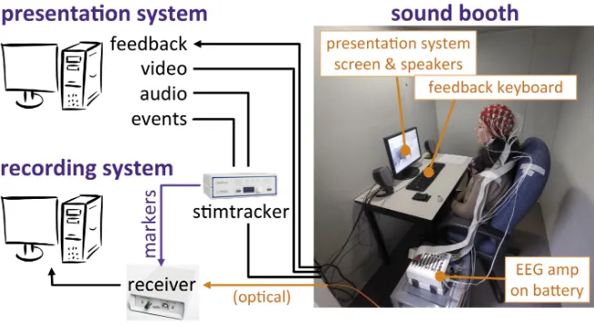
For the EEG portion of the study, the 10 participants sat in an audiometric room (Eckel model

CL-13). A BioSemi Active-Two system with 64+2 EEG channels recorded EEG data at 512 Hz as shown in Figure 2.1. Horizontal and vertical EOG channels recorded eye movements.

Figure 2.1: Setup for the EEG experiment. The presentation and recording systems were placed outside to reduce the impact of electrical line noise that could be picked up by the EEG amplifier.

The presented audio was routed through a Cedrus StimTracker connected to the EEG receiver,

which allowed a high-precision synchronization (<0.05 ms) of the stimulus onsets with the

EEG data. The experiment was programmed and presented using PsychToolbox run in Matlab

2014a. A computer monitor displayed the instructions and fixation cross for the participants

to focus on during the trials to reduce eye movements. The stimuli and cue clicks were played

through two tabletop speakers (Altec Lansing VS2121) at a comfortable level that was kept

constant across participants. Headphones were not used because pilot participants reported

2.3. Equipment andProcedure 11

of the experiment. After the experiment, we asked participants the method they used to imagine

the music stimuli. The participants were split evenly between imagining themselves producing

the music (singing or humming) and simply “hearing the music in [their] head.”

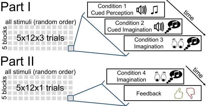
The EEG experiment was divided into 2 parts with 5 blocks each as illustrated in Figure 2.2.

A single block comprised all 12 stimuli in randomized order. Between blocks, participants

time

Condition 1

Cued Perception

♫

Part I

Part II

5x12x3 trials

all stimuli (random order)

5x12x1 trials

5

bl

ocks

all stimuli (random order)

Figure 2.2: Illustration of the design for the EEG portion of the study.

12 Chapter2. Methods

We recorded EEG in 4 conditions:

1. Stimulus perception preceded by cue clicks

2. Stimulus imagination preceded by cue clicks

3. Stimulus imagination without cue clicks

4. Stimulus imagination without cue clicks, with feedback

Conditions 3 and 4 simulate a more realistic query scenario during which the participant

has not heard the stimulus immediately prior to imagining. Conditions 3 and 4 were identical

except for the trial context. While the condition 1–3 trials were recorded directly back-to-back

within the first part of the experiment, all condition 4 trials were recorded separately in the

second part without any cue clicks or tempo priming by prior presentation of the stimulus.

After each condition 4 trial, participants provided feedback by pressing one of two buttons

indicating whether or not they felt they had imagined the stimulus correctly. In total, 240 trials

(12 stimuli x 4 conditions x 5 blocks) were recorded per subject.

2.4

Preprocessing

The raw EEG and EOG data were preprocessed using the MNE-Python toolbox. Channels

containing noise that could not be removed by simple filtering techniques (i.e., resulting from

muscle movements or bad electrical contact with scalp) were identified as ‘bad’ by visual

inspection. The bad channels were removed and interpolated (between 0 and 3 per subject). For

2.4. Preprocessing 13

data were then filtered with an overlap-add FIR filter (filter length 10s), keeping a frequency

range between 0.5 and 30 Hz. The width of the transition band was 0.1 at 0.5Hz and 0.5 at

30Hz. The filtering removed unwanted high frequency information and any slow signal drift in

the EEG. Removing unwanted noise (i.e. from external sources or muscle movements) restricts

analyses to data within the frequency range of signals produced by the brain. We computed

independent components using extended Infomax independent component analysis (ICA) (Lee,

Girolami, & Sejnowski, 1999) and removed components that had a high correlation with the

EOG channels to remove artifacts caused by eye blinks. This ensured that the final results could

be attributed to brain responses, not other sources of electrical activity. Finally, the data from

the 64 EEG channels were reconstructed from the remaining independent components. The

data from two participants were rejected during preprocessing due to excessive noise caused

Chapter 3

ERP Analysis

Our first analysis of the data followed a strategy similar to the one used in Schaefer et al. (2011).

Schaefer et al. (2011) used short stimuli (3.26s) allowing each stimulus to be repeated many

times and the data to be averaged across hundreds of short trials. The grand average ERPs were

concatenated to create one long data set and subjected to a PCA, yielding clearly defined spatial

features. The differences in the time courses of these components were used to classify their stimuli. We tried to replicate these results, using the time courses of components derived from

the average of the first 3.26 seconds of each of our stimuli. We were unable to achieve

signifi-cant classification results, likely because of our small number of stimuli repetitions. Therefore,

to preserve as much data as possible, we conducted a second PCA using the full length of the

trials as opposed to the first 3.26 seconds. We computed grand average ERPs for each stimulus

by averaging the full length trials (excluding the cue). We then concatenated the grand average

ERPs and applied a PCA. This resulted in principal components with poorly defined spatial

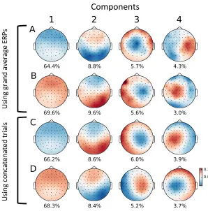
components in Figure 3.1 (A and B).

When we calculated grand average ERPs, some of the data was lost which could have

negatively impacted the PCA results. To preserve as much of the data as possible, we took

an alternative approach. All of the raw trials, rather than the averages, were concatenated to

create a single, long trial that contained all of the raw EEG information. We ran a PCA on the

concatenated raw trials. This produced clearly defined spatial components Figure 3.1 (C and

15

Components

Figure 3.1: Topographic visualization of the top 4 principal components with percentage of the explained signal variance. Channel positions in the 64-channel EEG layout are shown as dots. Colors are interpolated based on the channel weights. The PCA was computed onA: the grand average ERPs of all perception trials;B: the grand average ERPs of all cued imagination trials; C: the concatenated perception trials;D: the concatenated cued imagination trials.

D). Except for their (arbitrary) polarity, the components are very similar across perception and

imagination, which replicates the results found in (Schaefer et al., 2011).

To investigate how similar these components were across conditions and stimuli, we

corre-lated the time courses of component three during perception and imagination. We used

compo-nent three as it accounted for the most variance while being most similar to a typical auditory

component (peak in the fronto-central region of the topographic spatial map). The correlation

16 Chapter3. ERP Analysis

near the beginning of the trial, before participants’s imagination had a chance to drift too far

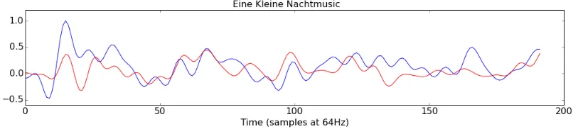
from the cued tempo. The highest correlations produced by this component werer(190)=0.40 (p<0.001) for “Eine Kleine Nachtmusic” (Figure 3.2) and r(190)= 0.30 (p<0.001) for “The

Figure 3.2: The time course of component three during perception (blue) and imagination (red) of Eine Kleine Nachtmusic. The correlation between the two time courses is r(190) = 0.40 (p<0.001).

Emperor Waltz” (Figure 3.3). Although these correlations seem promising for stimulus

classi-Figure 3.3: The time course of component three during perception (blue) and imagination (red) of The Emperor Waltz. The correlation between the two time courses is r(190) = 0.30 (p<0.001).

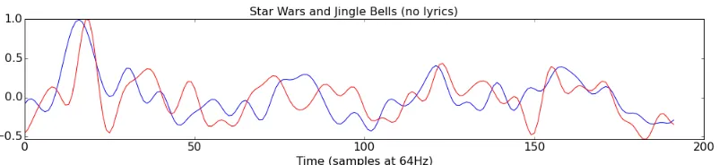
fication, the highest correlation ofr(190)=0.52 (p<0.001) occurred between the imagination of Jingle Bells (without lyrics) and the perception of the Star Wars theme Figure 3.4. The

high correlation between unrelated stimuli indicated that the component time course was not

tracking the brain’s unique response to each stimulus. Instead, it may be representative of more

17

Figure 3.4: The time course of component three during perception (blue) of the Star Wars theme and imagination (red) of Jingle Bells (no lyrics). The correlation between the two time courses isr(190)=0.52 (p<0.001).

occurred between trials from different stimuli we could not use this approach to classify our stimuli.

Our inability to accurately classify stimuli using the time courses of components could be

caused by recording fewer trials than Schaefer et al. (2011). We collected fewer trials per

stimulus because the end-goal was to build a music-based BCI to be used with patients. We

wanted to investigate the possibility of developing a BCI that would use minimal training which

would reduce the risk of training fatigue in patients. We only had 5 trials per stimulus, ranging

from 6.9s to 16s, while Schaefer et al. (2011) collected 145 trials of each of their stimuli, each

Chapter 4

Neural Network

Schaefer et al. (2011) were able to use the unique time course of the component responsible

for the most variance to differentiate between stimuli. With our components we were unable to reproduce this stimulus classification accuracy.

To classify our data, we used a technique from computer science called a convolutional

neural network (CNN). A CNN contains one or more convolutional layers that process the

data. In these layers, the input was processed by a filter (weight matrix) that was trained

using backpropagation (Rumelhart, Hinton, & Williams, 1986). The same filter was applied

at different positions (time points) of the input. Our network was optimized for our stimulus classification task and included three processing layers. The first layer was pre-trained on the

perception data using 384 trials (8 subjects x 12 stimuli x 4 trials) and then was not changed

during training of the full 3-layer model. One trial of each stimulus from each subject’s data

was left out to be used as the test set for later model testing (96 trials (8 subjects x 12 stimuli

x 1 trial) ). The full explanation of how we arrived at the best model can be found in (Stober,

Sternin, Owen, & Grahn, 2016) (arXiv:1511.04306).

4.1. Layer1: SimilarityConstraintEncoding 19

4.1

Layer 1: Similarity Constraint Encoding

We wanted to find features in the data that were stable across trials and subjects, and also

dis-tinguished between classes. To identify such features, we used a pre-training strategy called

similarity-constraint encoding. As introduced by Schultz and Joachims (2004), a relative

sim-ilarity constraint (a,b,c) describes a relative comparison of the trialsa,b, andcin the form “a

is more similar to bthan ais to c.” Here, ais the reference trial used for this comparison, b

is a trial from the same stimulus, and cis a trial from another stimulus. The number of

vio-lated constraints is used as a cost function for learning features of the data that are important

for stimulus classification. A cost function describes the characteristics of the system that we

want to minimize – in this case we want to minimize the number of violations to the similarity

constraint.

To this end, we combined all pairs of trials (a,b) from the same stimulus with all trials

c from other stimuli. During supervised learning, the system was forced to learn features of

the data constrained byaandbbeing more similar thana andc. For example, we created all

possible pairs of trials from the perception of Jingle Bells with lyrics and then combined each

of those pairs with all other perception trials. Each one of these triplets was then processed by

the similarity constraint encoder (SCE). The SCE learned features, in this case EEG channel

weights, that, when applied to the EEG trials, produced representations of each one of the

trials in the triplet. The representations were compared using the dot product as a similarity

measure. Each triplet produced two similarity scores: one comparing a and b (trials from

20 Chapter4. NeuralNetwork

constraint, the similarity score betweenaandbmust be higher thanaandc.

During training, the number of violated constraints was minimized using

backpropaga-tion and stochastic gradient descent with a learning rate momentum (Rumelhart, Hinton, &

Williams, 1988). In this scenario, backpropagation allowed the SCE to update its learned

fea-tures (channel weights) to produce representations of the trials that satisfied the constraint. To

help the SCE hone in on the optimal learned features, stochastic gradient descent forced the

learned features to be updated in the direction of minimizing the violations of the constraint.

Learning rate momentum is a method to improve the performance of stochastic gradient

de-scent by controlling how the model’s parameters are modified. Rather than the features

(chan-nel weights) being updated after each triplet was processed, the features were updated after

128 trials (referred to in the literature as a ‘mini-batch’) had been processed. The final features

learned by the SCE were more similar for trials from the same stimulus than for trials from

different stimuli.

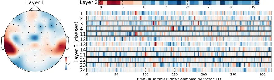
The spatial pattern of the features learned by this SCE is visualized in Layer 1 of

Fig-ure 4.1. The coloFig-ured areas represent the regions and the electrode weightings that the encoder

has determined are optimal for differentiating stimuli. This pattern acts as a spatial filter that processes the raw data. The 64 EEG channels are reduced to a single data stream of weighted

EEG by this filter1_.

1_{After being processed by the spatial filter we applied a non-linear activation function to the data (a step which}

4.2. Layer2: TemporalFilter& Layer3: Templates 21

Layer 3 (classes)

Layer 1

-0 +

0 5 10 15 20 25 30 35

Layer 2

1

2

3

4

11

12

13

14

21

22

23

0 50 100 150 200 250 300

time (in samples, down-sampled by factor 11)

24

Figure 4.1: Visualization of our neural network, which processes raw EEG at a sampling rate of 512 Hz. Layer 1 was pre-trained using similarity-constraint encoding and is a spatial repre-sentation of EEG electrode weights. Layer 2 is a 37 sample long temporal filter. Layer 3 shows the compressed representations of the raw EEG data. The numbers are the ID numbers of the stimuli found in Table 2.1. The colours are an indication of the weighting decided on by the model. We can interpret the intense red and blue colours as being more important for stimulus classification than the white areas.

4.2

Layer 2: Temporal Filter & Layer 3: Templates

Layers two and three were trained together with supervised learning and optimized by

back-propagation through the entire model with a cost function to minimize classification error. The

single data stream output from layer one entered the second layer where it was convolved with

the filter (step size of 1). The resulting output was then pooled over 21 samples with a step size

of 11. This produced a compressed representation of the EEG data.

To find the optimal parameters (learning rate, filter size, etc.) for our neural network, we

employed a 8-fold cross validation scheme by training on the data from 8 subjects (384 trials)

and validating on the remaining subject (48 trials). The cross-validation was done within the

training set. The final versions of layer 2 and 3 seen in Figure 4.1 are an average of the model

22 Chapter4. NeuralNetwork

and layer 3 contains a temporal pattern that was learned from the output of layer 2 and is a

compressed representation of the EEG data.

4.3

Full model explanation

The classification accuracy of the model was then tested with the test set of 96 trials. Each

trial in the test set was processed by the filters in layer 1 and layer 2. The resulting

com-pressed representation (the output from layer 2) of the test trial was compared against each

of the optimized temporal patterns in layer 3 of the model. The dot product of the test trial’s

representation was taken with each of the optimized layer 3 patterns. This produced 12 values

(one for each stimulus) that described the similarity of the test trial’s representation with each

of the optimized patterns. Using the dot product as a similarity measure, the test trial was given

4.4. Results 23

4.4

Results

First, we tested the model with the perception data. Significance values were determined by

using the cumulative binomial distribution to estimate the likelihood of observing a given

clas-sification rate by chance (Combrisson & Jerbi, 2015). Using the cumulative binomial

distribu-tion allows us to determine the number of observadistribu-tions that are correctly classified by chance

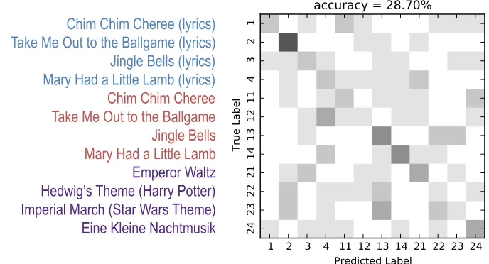
with respect to the number of observations. Our model was able to classify the 12-classes (12

stimuli listed in Table 2.1) with a 28.7% accuracy rate (chance = 17.59%) at a significance level of p=0.001. Figure 4.2 is a confusion matrix which shows the classification results for each stimulus. From the confusion matrix we can see that some stimuli were more accurately

12-Class Stimuli Confusion

2015-12-01

Sebastian Stober - Deep Feature Learning for EEG 51

Chim Chim Cheree (lyrics) Take Me Out to the Ballgame (lyrics) Jingle Bells (lyrics) Mary Had a Little Lamb (lyrics)

Chim Chim Cheree Take Me Out to the Ballgame Jingle Bells Mary Had a Little Lamb

Emperor Waltz Hedwig’s Theme (Harry Potter) Imperial March (Star Wars Theme) Eine Kleine Nachtmusik

Figure 4.2: 12-class confusion matrix for perception data. The numbers along the axes cor-respond to the ID numbers of the stimuli found in Table 2.1. Intensity indicates the number of times a true label was classified as a predicted label with darker colours indicating more classifications.

classified than others. Stimulus 2 (Take Me Out to the Ballgame with lyrics) is the most

24 Chapter4. NeuralNetwork

their lyric counterparts (stimuli 3 and 4) can be seen. Confusion between lyric and non-lyric

pairs can also be seen with stimulus 1 being classified as stimulus 11.

To further investigate which pairs of stimuli the classifier could distinguish best, we put

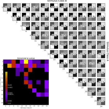
all combinations of paired stimuli through our classifier. This resulted in the series of binary

confusion matrices in Figure 4.3 that show us that some pairs of stimuli are more easily

dif-ferentiated than others. Within each binary confusion matrix chance is 66.67% (alpha=0.05). 1 2 2 3 3 4 4 11 11 12 12 13 13 14 14 21 21 22 22 23 23 24

2 3 4 11 12 13 14 21 22 23 24

Stimulus Class B 1 2 3 4 11 12 13 14 21 22 23

Stimulus Class A

Stimulus Class B

Stimulus Class A

binomial p-value 0.01 0.005 0.00075 0.0005 0.0001 5e-05

4.4. Results 25

For example: Chim Chim Cheree with lyrics is classified correctly 100% of the time when

paired with Jingle Bells without lyrics. The statistical significance (p-value) of each of the

comparisons is visualized in the figure’s inset.

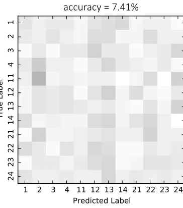
The imagination data was then tested on the same model (i.e. there was no additional

training using the imagination data). The model was not able to classify the 12 stimuli from

the EEG data collected during music imagination. Figure 4.4 is a confusion matrix which

shows the imagination classification results at 7.41% (below chance=12.96%, alpha=0.05). As can be seen in the figure, there is no clear pattern to the confusion indicating that the system

was not making classification errors in a systematic way.

12-Class Stimuli Confusion

2015-12-01

Sebastian Stober - Deep Feature Learning for EEG 51

Chim Chim Cheree (lyrics) Take Me Out to the Ballgame (lyrics) Jingle Bells (lyrics) Mary Had a Little Lamb (lyrics) Chim Chim Cheree Take Me Out to the Ballgame Jingle Bells Mary Had a Little Lamb

Emperor Waltz Hedwig’s Theme (Harry Potter) Imperial March (Star Wars Theme) Eine Kleine Nachtmusik

accuracy = 7.41%

Figure 4.4: 12-class confusion matrix for imagination data. The numbers along the axes cor-respond to the ID numbers of the stimuli found in Table 2.1. Intensity indicates the number of times a true label was classified as a predicted label with darker colours indicating more classifications.

We investigated whether there were pairs of imagined stimuli that the classifier could

26 Chapter4. NeuralNetwork

at a statistically significant level.

1 2 2 3 3 4 4 11 11 12 12 13 13 14 14 21 21 22 22 23 23 24 2 3 4 11 12 13 14 21 22 23 24

Stimulus Class B 1 2 3 4 11 12 13 14 21 22 23

Stimulus Class A

Stimulus Class B

Stimulus Class A

binomial p-value 0.05 0.01 0.005 0.00075 0.0001

4.5. Discussion 27

4.5

Discussion

The neural net does not give us information about what characteristics from the EEG it used

to classify the stimuli, and it is difficult to interpret from the results what signals the brain is producing that allow this classification to occur. In layer 3 of Figure 4.1 we see compressed

representations of the EEG data for each stimulus. One characteristic of these representations

is the dark red vertical bands that stand out from the rest of the time course. These red bands

indicate time periods that the neural net has identified as being important for classifying the

stimuli. When taking a closer look, we see that these bands occur at the same time point for

lyric/non-lyric pairs of stimuli. For example, the darkest red band in stimulus 1 (Chim Chim Cheree with lyrics) appears at a very similar time point as the darkest red band in stimulus 11

(Chim Chim Cheree without lyrics). A similar pattern can be seen for stimuli 2/12 and 3/13. Upon investigation of the audio of the stimuli at these time periods, there were no

characteris-tics (e.g. lyric repetition, important music moments, end of phrases, change in dynamics, etc.)

that stood out as driving these moments to be labeled as important. These red bands may

repre-sent a cognitive process, such as recognition, that occurs at these time points during perception

of the stimuli. To investigate this possibility, we ran a follow-up behavioural experiment asking

participants to indicate when they consciously recognized each stimulus. This experiment is

described in the next section.

The results of our neural net show that some stimuli are better classified than others, and

28 Chapter4. NeuralNetwork

asking participants to rate the similarity of pairs of stimuli. The results will tell us whether the

Chapter 5

Behavioural Experiment

We ran a follow-up experiment to learn more about what information from the EEG data the

neural net used to classify the stimuli. First, we investigated whether the vertical red bands

from layer 3 (Figure 4.1) were associated with a cognitive process that may have supported the

neural net’s classification, such as recognition of the music. Then, we investigated whether the

neural net confused stimuli that were rated as highly similar by humans.

5.1

Participants

Nine participants (four male), aged 22-28, with normal hearing and no history of head injuries

took part in this study. Six participants had formal music training (2-15 years), and four of

those participants played instruments regularly at the time of data collection.

5.2

Procedure

The 12 stimuli were the same songs as those in the original experiment (See Table 2.1). The

experiment had two parts and lasted about 50 mins. First, participants listened to each of the

12 stimuli and pressed a button when (and if) they recognized the piece of music. The timing

of their key press was recorded. During the second part of the experiment, participants were

30 Chapter5. BehaviouralExperiment

presented with all possible paired combinations of stimuli (78 pairs). They listened to the first

song followed immediately by the second, and then rated how similar the two songs sounded

on a scale from 0 - 100 (0=the songs sound nothing alike, 100=the songs sound exactly the same). Participants were given the following instructions:

Different pieces of music can sound similar or different for many reasons. For

example, different songs may sound similar if sung by the same person, or played

on the same instrument. Other times, the same song might sound very different

when sung by different people or played on different instruments. During this

experiment you will hear pairs of songs and rate how similar they sound to you.

You should focus on how generally similar the songs feel to you. Don’t worry

about whether you are correct or not.

5.3

Results

To determine whether the periods of time highlighted by the neural net in layer 3 of Figure 4.1

(vertical red bands) are related to a cognitive process, such as recognition, we collected the

average time at which people recognized these musical pieces (Figure 5.1). Based on these

results, the highlighted time periods from layer 3 of the neural net were unrelated to the time

at which people recognized the piece of music.

To determine whether the neural net confused songs that humans rated as similar,

partic-ipants rated pairs of songs on similarity. Figure 5.2 shows the similarity rating results. As

5.3. Results 31

Figure 5.1: Average time it takes for participants to recognize these stimuli (red). Individ-ual data is shown in black and song length is shown in blue. The magenta bars indicate the highlighted time periods from layer three in the neural net (Figure 4.2).

of songs were also rated as highly similar, and that is seen in the four, dark squares that are

parallel to the diagonal.

The classification accuracy values produced by the neural network in the confusion matrix

in Figure 4.3 can be interpreted as “dissimilarity” scores, so we took their inverse (100 - score)

to produce similarity scores, and correlated the similarity matrix with the similarity ratings

32 Chapter5. BehaviouralExperiment

Similarity Ratings

1 2 3 4 11 12 13 14 21 22 23 24

Song 1

1

2

3

4

11

12

13

14

21

22

23

24

Song 2

10 20 30 40 50 60 70 80 90

Chapter 6

Discussion

The goal of these experiments was to investigate whether the perception and imagination of

short musical pieces could be classified from EEG data. The ability to classify musical pieces

from imagination could lead to the development of a BCI that would allow patients with motor

deficits to communicate through music imagination. Ideally, patients would be able to imagine

a piece of music to convey a certain thought (i.e. imagining “Jingle Bells” to indicate hunger).

Schaefer et al. (2011) were able to classifyperceived music stimuli based on the unique time

courses of principal components that occurred during music perception, but we were unable to

achieve the same result. The most likely reason is the number of stimuli presented to

partici-pants, as we presented far fewer trials per stimulus (5 vs 145). The small number of trials is

also likely responsible for our inability to classify imagination using either the PCA technique

or machine learning.

The rationale for including so few trials per stimulus stemmed from the end-goal of building

a music-based BCI. A BCI must operate with as little training as possible when used with

patients. The patients that require such interfaces to communicate may have difficulty directing attention, and focusing on a single task for a long time can be exhausting. A system that

requires minimal training cuts down on patient fatigue during the training stage, ensuring that

patients have enough energy to use the system for communication. Ideally, our BCI would be

trained on brain data collected during theperceptionof music and tested on brain data collected

34 Chapter6. Discussion

duringimaginationof music. By training on perception data we hoped to keep patient fatigue

to a minimum. However, our results indicated that this is currently not a viable option with the

existing data.

Using machine learning techniques, we were able to train our system and classify the

per-ception of music stimuli from the recorded EEG signal at a 28.7% accuracy rate (chance = 17.59%). When investigating the pairs of stimuli that were most easily classified, there was

no relationship to the energy attribute (calculated using EchoNest) of each musical piece (i.e.,

pieces with the most different energy levels were not more easily classifed). When applied to data collected during imagination of music, our neural network failed. The confusion

ma-trix produced by the network (Figure 4.4) is similar to what one would expect when trying

to classify noise. This result indicates that the system was not systematically misclassifying

stimuli.

There are multiple reasons that could explain why we were unable to classify music

imag-ination. During perception, the timing of the music is consistent across trials (e.g. the second

beat of the song always occurs at a consistent time point) because the timing is driven by the

stimulus. During imagination, this timing may fluctuate across trials and across participants,

because after the end of the tempo cue there is no external stimulus. A single participant may

imagine music at a different rate on different trials, and some participants may have a tendency to speed up or slow down throughout their imagining. Another inconsistency that may occur

across participants, and across trials, is the focus of the imagination. It is possible that

35

choose to imagine the melody, the lyrics, or the instrumentation, and their focus may shift

across trials. There are also differences in ‘how’ participants imagine music. After the exper-iment was completed, we asked participants what technique they used to imagine the music.

There was a 50-50 split between participants imagining themselves producing the music (i.e.

singing the music) and participants “hearing the music in their head”. Some participants also

reported imagining vivid scenes, either from existing movies or completely novel scenes, to

illustrate their music imagination. This wide array of differences is likely the cause of our low imagination classification rates.

The secondary goal of these experiments was to determine what neural processes drive the

classification of music perception and imagination. Although it is tempting to interpret the

results of a neural network, it is difficult to determine why a trained neural network makes a particular decision (Towell & Shavlik, 1992). One way of understanding a neural network’s

de-cisions is by investigating the layers of the network separately and relating the weights within

these layers to the input and the output. However, understanding the structure of a neural

net-work may not necessarily inform us about what the brain is doing to perform the same task.

First, the network’s solution may not be unique and may simply be one of many possible

so-lutions. Although the network is constrained to minimize misclassification error, the solution

reached by the network could be a local minimum – the best solution for this particular

com-bination of parameters. The network tries out different combinations of parameters until it finds a solution that it decides best minimizes misclassification error. However, with further

36 Chapter6. Discussion

that minimizes the misclassification error further. It is impossible to know whether the

net-work’s solution is the global minimum – the solution with the lowest possible misclassification

error. Second, interpretation is difficult because a solution is reached based on parameters set by the researcher. It is not possible to untangle whether aspects of the solution are necessary

for solving the problem or if they are influenced by the chosen network architecture. Lastly,

convolutional neural networks, like the one used in this experiment, are artificial, and only

superficially resemble the way a biological system processes information. It is not possible

to know whether the way an artificial network solves a biological problem is the same way a

biological system would solve it.

However, to investigate whether we could glean any brain-related information from our

neural network (Figure 4.1), we focused on whether the spatial or temporal filters could be

related to any biological or musical characteristics. The spatial filter in layer 1 indicated which

electrodes carried the EEG data important for classification. However, because of the spatially

imprecise nature of EEG, we are unable to comment on where the data from these electrodes

is produced. EEG collects electrical signals at the scalp that are produced by the brain. By the

time the electrical information reaches the electrodes, it has travelled through layers of tissue

and the skull and is diffuse. Trying to reconstruct the sources of the electrical signal in three dimensional space presents a reverse inference problem with countless solutions. Because

there is more than one way to identify sources within the brain that could produce the electrical

37

One approach to breaking an EEG signal down into constituent parts is to use PCA. The

auditory research literature is in consensus on what principal components of auditory

process-ing look like. However, the spatial filter in layer 1 does not match what is seen in a PCA of

auditory EEG. Generally auditory component peaks are located in the fronto-central region of

the topographic spatial map. The layer 1 filter does not have any similarities to the biologically

produced components and has lateral peaks. Because we could not relate the layer 1 filter to

any biological information, and we had no way to interpret what type of signals are picked up

by the electrodes the model has labeled as important for classification, we decided to force the

net to use biologically produced information to see whether the model’s classification abilities

change. We exchanged the neural net’s first layer with the principal components calculated in

Figure 3.1C. This resulted in a decrease in classification accuracy. The results from the neural

net using biologically produced spatial maps can be seen in Appendix C.

The second and third layers of the neural net produced temporal filters and compressed

representations of the data that highlight time periods in the stimuli that are important for

clas-sification. Upon closer investigation there were no auditory characteristics that stood out as

being unique to each of the important time periods. These time periods did not relate to salient

auditory events, important points in the musical structure of the piece, or any obvious aspect of

the lyrics, such as word repetition. To determine whether the patterns in the filters were driven

by a cognitive process such as recognition of the music we conducted a behavioural

experi-ment. The results showed that the highlighted time periods do not coincide with the moment

rec-38 Chapter6. Discussion

ognize the pieces of music well before the important time periods occur in the temporal filters.

Based on these results we know what isnotresponsible for highlighting these moments in the

classifier: the importance of these moments is not due to auditory characteristics of the

stim-uli or a moment of recognition. At this time we are unable to say what is causing these time

periods to be flagged as important for stimulus classification.

Although we were able to classify music perception (accuracy=28.7%), we were not able to classify music imagination (accuracy = 7.4%). Future experiments should aim to disen-tangle what information is driving the classifier during perception and to enhance this during

imagination. To do this we may need to use simpler stimuli. Rhythm stimuli are simpler than

music stimuli because they do not include melody, lyric, or instrumentation information. If we

are able to classify the imagination of rhythmic stimuli more accurately than the imagination

of music then we may be able to say that it is the rhythmic component of music driving the

classification in this experiment. Then, one at a time, we can add in other aspects of music like

tone and lyrics to determine what effect they have on classification accuracy until we reach the optimum combination of musical characteristics. Previous research has shown that it is

possi-ble to classify the perception of rhythms (Stober, Cameron, & Grahn, 2014a), so capitalizing

on rhythm’s auditory simplicity may be an effective way to learn what characteristics are nec-essary to drive a music-based BCI. Finally, it will also be important during future experiments

to continue to cue participants to the tempo during imagination using a metronome. This will

References

Cirelli, L. K., Bosnyak, D., Manning, F. C., Spinelli, C., Marie, C., Fujioka, T., . . . Trainor, L. J. (2014). Beat-induced fluctuations in auditory cortical beta-band activity: Using EEG to measure age-related changes.Frontiers in Psychology,5(Jul), 1–9. doi: 10.3389/ fpsyg.2014.00742

Combrisson, E., & Jerbi, K. (2015). Exceeding chance level by chance: The caveat of theoret-ical chance levels in brain signal classification and statisttheoret-ical assessment of decoding ac-curacy. Journal of Neuroscience Methods, 1–11. doi: 10.1016/j.jneumeth.2015.01.010 Ellis, D. P., Whitman, B., Jehan, T., & Lamere, P. (2010). The echo nest musical

finger-print. InIsmir 2010 utrecht: 11th international society for music information retrieval conference, august 9th-13th, 2010.

Fujioka, T., Trainor, L. J., Large, E. W., & Ross, B. (2009). Beta and gamma rhythms in human auditory cortex during musical beat processing.Annals of the New York Academy of Sciences,1169, 89–92. doi: 10.1111/j.1749-6632.2009.04779.x

Fujioka, T., Trainor, L. J., Large, E. W., & Ross, B. (2012). Internalized timing of isochronous sounds is represented in neuromagnetic beta oscillations.Journal of Neuroscience,32(5), 1791–1802. doi: 10.1523/JNEUROSCI.4107-11.2012

Geiser, E., Ziegler, E., Jancke, L., & Meyer, M. (2009). Early electrophysiological correlates of meter and rhythm processing in music perception. Cortex,45(1), 93–102. doi: 10.1016/ j.cortex.2007.09.010

Halpern, A. R., Zatorre, R. J., Bouffard, M., & Johnson, J. A. (2004). Behavioral and neural correlates of perceived and imagined musical timbre. Neuropsychologia, 42(9), 1281– 92. doi: 10.1016/j.neuropsychologia.2003.12.017

Herholz, S., Halpern, A., & Zatorre, R. (2012). Neuronal correlates of perception, imagery, and memory for familiar tunes. Journal of cognitive neuroscience,24(6), 1382–97. doi: 10.1162/jocn\ a\ 00216

Herholz, S., Lappe, C., Knief, A., & Pantev, C. (2008, December). Neural basis of music imagery and the effect of musical expertise. The European journal of neuroscience,

28(11), 2352–60. doi: 10.1111/j.1460-9568.2008.06515.x

Iversen, J. R., Repp, B. H., & Patel, A. D. (2009). Top-down control of rhythm perception modulates early auditory responses. Annals of the New York Academy of Sciences,1169, 58–73. doi: 10.1111/j.1749-6632.2009.04579.x

Kalat, J. W. (2008). Neural Basis of Visual Perception. InBiological psychology(10th ed., pp. 165–179). Wadsworth Publishing.

Kraemer, D. J. M., Macrae, C. N., Green, A. E., & Kelley, W. M. (2005, March). Musical imagery: sound of silence activates auditory cortex. Nature, 434(7030), 158. doi: 10 .1038/434158a

Lee, T.-W., Girolami, M., & Sejnowski, T. J. (1999). Independent component analysis using an extended infomax algorithm for mixed subgaussian and supergaussian sources. Neural Computation,11(2), 417–441. doi: 10.1162/089976699300016719

Merchant, H., Grahn, J., Trainor, L. J., Rohrmeier, M., & Fitch, W. T. (2015). Finding a beat: a

40 References

neural perspective across humans and non-human primates. Philosophical Transactions of the Royal Society B: Biological Sciences.

Monti, M. M., Vanhaudenhuyse, A., Coleman, M. R., Boly, M., Pickard, J. D., Tshibanda, L., . . . Laureys, S. (2010). Willful Modulation of Brain Activity in Disorders of Conscious-ness. The New England Journal of Medicine(362), 579–589.

M¨ullensiefen, D., Gingras, B., Musil, J., & Stewart, L. (2014). The musicality of non-musicians: An index for assessing musical sophistication in the general population.PLoS ONE,9(2). doi: 10.1371/journal.pone.0089642

Nozaradan, S., Peretz, I., Missal, M., & Mouraux, A. (2011). Tagging the neuronal entrainment to beat and meter. The Journal of Neuroscience, 31(28), 10234–10240. doi: 10.1523/ JNEUROSCI.0411-11.2011

Perrin, F., Pernier, J., Bertrand, O., & Echallier, J. F. (1989). Spherical splines for scalp potential and current density mapping. Electroencephalography and Clinical Neuro-physiology,72(2), 184–187. doi: 10.1016/0013-4694(89)90180-6

Rumelhart, D. E., Hinton, G. E., & Williams, R. J. (1986). Learning representations by back-propagating errors. Nature,323(6088), 533–536. doi: 10.1038/323533a0

Rumelhart, D. E., Hinton, G. E., & Williams, R. J. (1988). Learning representations by back-propagating errors. Cognitive modeling,5(3), 1.

Schaefer, R. S. (2011). Measuring the mind’s ear: EEG of music imagery (Unpublished doctoral dissertation). Radboud University Nijmegen.

Schaefer, R. S., Blokland, Y., Farquhar, J., & Desain, P. (2009). Single trial classification of perceived and imagined music from EEG. In Proceedings of the 2009 Berlin BCI Workshop.

Schaefer, R. S., Desain, P., & Farquhar, J. (2013). Shared processing of perception and imagery of music in decomposed EEG. NeuroImage, 70, 317–326. doi: 10.1016/j.neuroimage .2012.12.064

Schaefer, R. S., Farquhar, J., Blokland, Y., Sadakata, M., & Desain, P. (2011). Name that tune: Decoding music from the listening brain. NeuroImage, 56(2), 843–849. doi: 10.1016/j.neuroimage.2010.05.084

Schultz, M., & Joachims, T. (2004). Learning a distance metric from relative comparisons.

Advances in neural information processing systems (NIPS), 41–48.

Snyder, J. S., & Large, E. W. (2005). Gamma-band activity reflects the metric structure of rhythmic tone sequences. Cognitive Brain Research, 24, 117–126. doi: 10.1016/ j.cogbrainres.2004.12.014

Stober, S., Cameron, D. J., & Grahn, J. A. (2014a). Does the beat go on? – Identifying rhythms from brain waves recorded after their auditory presentation. In9th audio mostly: A conf. on interaction with sound (am’14)(pp. 23:1–23:8).

Stober, S., Cameron, D. J., & Grahn, J. A. (2014b). Using convolutional neural networks to recognize rhythm stimuli from electroencephalography recordings. In Advances in neural information processing systems 27 (nips’14)(pp. 1449–1457).

References 41

Towell, G., & Shavlik, J. W. (1992). Interpretation of artificial neural networks: Mapping knowledge-based neural networks into rules. In Advances in neural information pro-cessing systems(p. 977-984).

Vlek, R. J., Schaefer, R. S., Gielen, C. C. A. M., Farquhar, J. D. R., & Desain, P. (2011). Shared mechanisms in perception and imagery of auditory accents. Clinical Neurophysiology,

122(8), 1526–1532. doi: 10.1016/j.clinph.2011.01.042

Willander, J., & Baraldi, S. (2010). Development of a new clarity of auditory imagery scale.

Appendix A

Ethics Approval Form

Appendix B

Questionnaire

Participant Number:

Music Imagery Questionnaire

Date: Time:

Male⇤ Female⇤ Age:

Have you ever played and/or had formal training on any instrument (including vocal training)?

Yes⇤No⇤

If yes, indicate below which instruments, how long you played, and whether or not you still play.

Please include vocal training.

Instrument Number of years played I still play

⇤ ⇤ ⇤ ⇤ ⇤

Please circle the most appropriate category:

1. I engaged in regular, daily practice of a musical instrument (including voice) for 0 / 1 / 2 / 3 / 4-5 / 6-9 / 10 or moreyears.

2. At the peak of my interest, I practiced0 / 0.5 / 1 / 1.5 / 2 / 3-4 / 5 or morehours

per day on my primary instrument.

3. I have had formal training in music theory for0 / 0.5 / 1 / 2 / 3 / 4-6 / 7 or more

years.

4. I have had0 / 0.5 / 1 / 2 / 3-5 / 6-9 / 10 or more years of formal training on a

musical instrument (including voice) during my lifetime.

5. I listen attentively to music for 0-15min / 15-30min / 30-60min / 60-90min /

2hrs / 2-3hrs / 4hrs or moreper day.

6. I have music playing in the background for 0-15min / 15-30min / 30-60min /

60-90min / 2hrs / 2-3hrs / 4hrs or moreper day.

7. What device(s) do you most use to listen to music?

1