Classification with Large Sparse Datasets: Convergence Analysis and Scalable Algorithms

(1)

Western University Western University

Scholarship@Western

Electronic Thesis and Dissertation Repository

7-24-2017 12:00 AM

Classification with Large Sparse Datasets: Convergence Analysis

and Scalable Algorithms

Xiang Li

The University of Western Ontario Supervisor

Charles X. Ling

The University of Western Ontario Graduate Program in Computer Science

A thesis submitted in partial fulfillment of the requirements for the degree in Doctor of Philosophy

Follow this and additional works at: https://ir.lib.uwo.ca/etd

Part of the Artificial Intelligence and Robotics Commons, Statistical Models Commons, and the Theory and Algorithms Commons

Recommended Citation Recommended Citation

Li, Xiang, "Classification with Large Sparse Datasets: Convergence Analysis and Scalable Algorithms" (2017). Electronic Thesis and Dissertation Repository. 4682.

https://ir.lib.uwo.ca/etd/4682

This Dissertation/Thesis is brought to you for free and open access by Scholarship@Western. It has been accepted for inclusion in Electronic Thesis and Dissertation Repository by an authorized administrator of

(2)

Abstract

Large and sparse datasets, such as user ratings over a large collection of items, are common

in the big data era. Many applications need to classify the users or items based on the

high-dimensional and sparse data vectors, e.g., to predict the profitability of a product or the age

group of a user, etc. Linear classifiers are popular choices for classifying such datasets because

of their efficiency. In order to classify the large sparse data more effectively, the following important questions need to be answered.

1. Sparse data and convergence behavior. How different properties of a dataset, such as

the sparsity rate and the mechanism of missing data systematically affect convergence behavior

of classification?

2. Handling sparse data with non-linear model. How to efficiently learn non-linear data

structures when classifying large sparse data?

This thesis attempts to address these questions with empirical and theoretical analysis on

large and sparse datasets. We begin by studying the convergence behavior of popular classifiers

on large and sparse data. It is known that a classifier gains better generalization ability after

learning more and more training examples. Eventually, it will converge to the best

generaliza-tion performance with respect to a given data distribugeneraliza-tion. In this thesis, we focus on how the

sparsity rate and the missing data mechanism systematically affect such convergence behavior. Our study covers different types of classification models, including generative classifier and discriminative linear classifiers. To systematically explore the convergence behaviors, we use

synthetic data sampled from statistical models of real-world large sparse datasets. We consider

different types of missing data mechanisms that are common in practice. From the

experi-ments, we have several useful observations about the convergence behavior of classifying large

sparse data. Based on these observations, we further investigate the theoretical reasons and

come to a series of useful conclusions. For better applicability, we provide practical guidelines

for applying our results in practice. Our study helps to answer whether obtaining more data

or missing values in the data is worthwhile in different situations, which is useful for efficient data collection and preparation.

Despite being efficient, linear classifiers cannot learn the non-linear structures such as the low-rankness in a dataset. As a result, its accuracy may suffer. Meanwhile, most non-linear methods such as the kernel machines cannot scale to very large and high-dimensional datasets.

The third part of this thesis studies how to efficiently learn non-linear structures in large sparse data. Towards this goal, we develop novel scalable feature mappings that can achieve better

accuracy than linear classification. We demonstrate that the proposed methods not only

(3)

perform linear classification but is also scalable to large and sparse datasets with moderate

memory and computation requirement.

The main contribution of this thesis is to answer important questions on classifying large

and sparse datasets. On the one hand, we study the convergence behavior of widely used

classi-fiers under different missing data mechanisms; on the other hand, we develop efficient methods to learn the non-linear structures in large sparse data and improve classification accuracy.

Over-all, the thesis not only provides practical guidance for the convergence behavior of classifying

large sparse datasets, but also develops highly efficient algorithms for classifying large sparse datasets in practice.

Keywords: Machine learning, large-scale classification, data sparsity, classifier behavior

(4)

Acknowlegements

First of all, I would like to thank my supervisor, Dr. Charles Ling, who have guided me through

the path of becoming a better researcher and have taught me important lessons in doing solid

research. I am really grateful that Dr. Ling has always given me encouragement and actionable

suggestions when facing difficulties in research. Without his supervision, this thesis would not have been possible.

My gratitute also goes to my thesis committee members, Dr. Xianbin Wang, Dr. John

Barron, Dr. Michael Bauer and Dr. Xiaodan Zhu, who graciously agreed to serve on my

committee.

I would like to express my thanks to my lab members, Yan Luo, Shuang Ao, Jun Wang,

Chang Liu, Renfeng Liu, Xiao Li, Tanner Bohn for all the inspirations, encouragements and

help, in research and also in real life. Many thanks to Dr. Shuang Ao, we have many

coopora-tions in research and jointly published several papers. I would also like to thank Dr. Bin Gu,

who had been a visiting scholar to our lab in 2014. Since then, Dr. Gu has given me much

guidance in doing machine learning research, and we have coorporated in publication.

I would like to thank Dr. Huaimin Wang, the advisor of my Bachelor and Master study at

National University of Defense Technology. He recommended me to conduct doctoral study at

Western University and has always been supportive to me throughout my Ph.D. study.

Finally, my gratitude goes to my parents, for their love, sacrifice and tremendous support.

My research is supported by NSERC Grants, China Scholarship Council (CSC) and

Na-tional Natural Science Foundation of China (No. 61432020, 61472430). This thesis would not

have been possible without the generous resources provided by the Department of Computer

Science, Western University.

(5)

List of Figures

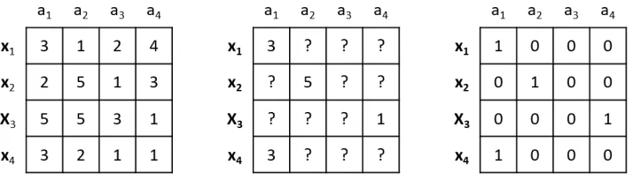
1.1 A toy dataset of four instances {x1,x2,x3,x4} and 4 features {a1,a2,a3,a4}.

From left to right: the full dataset in hindsight; the actually observed dataset

with 12 missing values (sparsitys=75%); and its missing pattern. . . 2

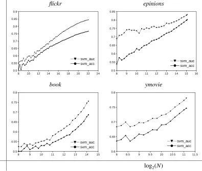
1.2 Learning curves of several real-world datasets measured by 5-fold cross-validation

accuracy and AUC. All data samplings are repeated for 5 times, the

regular-ization parameter of the SVM is tuned using a held-out dataset on the grid

[2−10,2−9, . . . ,210]. . . 4

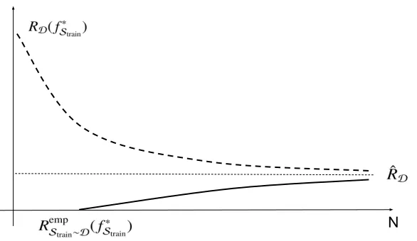
2.1 As the training sizeNincreases, the empirical risk (Remp_S

train∼D) and true risk (RD)

of a classifier f_S∗

train will converge. . . 12

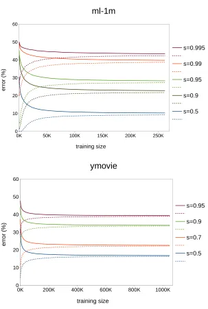
3.1 Training (dashed) and generalization error rates for different missing data prob-ability s. Observation: higher sparsity leads to larger asymptotic

generaliza-tion error rate. . . 25

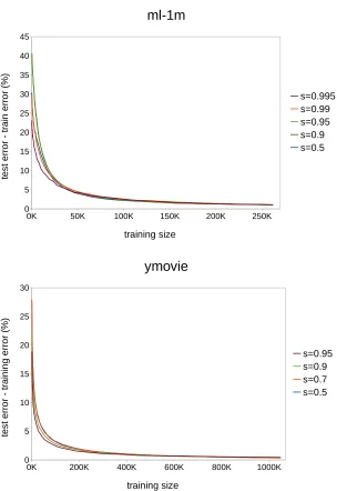
3.2 The difference between training and generalization error rates for different data missing probability s. Observation: asymptotic rate of convergence is almost

the same for different sparsity. . . 26

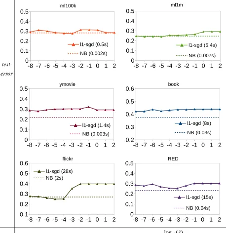
4.1 Classification error and CPU time comparison between Na¨ıve Bayes (NB) and

l1-regularized linear classifier (l1-sgd) on different user behavior datasets. The l1-regularized linear classifier is optimized with Stochastic Gradient Descent

with 107gradient updates. The x-axis is the logarithm scale of thel1-sgd

reg-ularization parameter λ. Observations: after careful parameter tuning

(sig-nificantly more CPU time), l1-sgd outperforms NB on 50% of the datasets;

However, NB gives lower error in most of the settings. . . 38

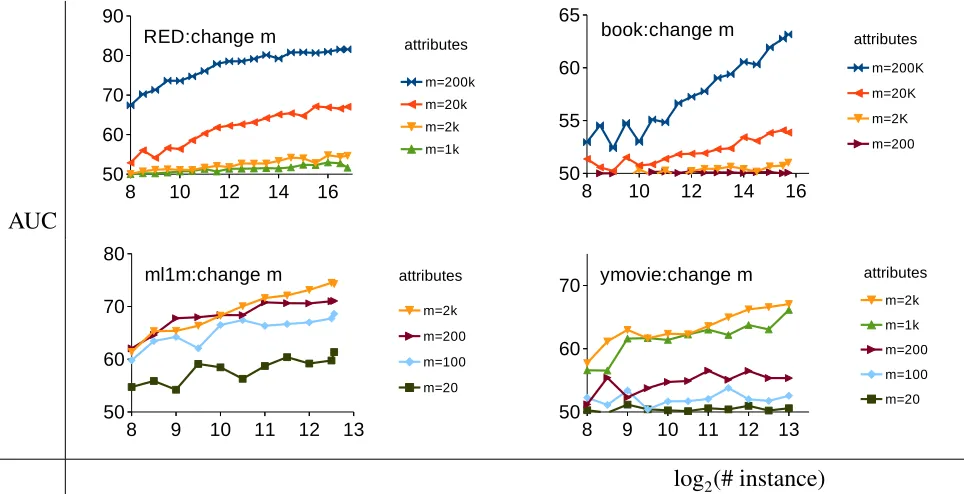
4.2 Na¨ıve Bayes AUC learning curves on real-world user behavior datasets as we

systematically varym. Observation: More attributes is always better, but we

cannot see the convergence behavior. . . 39

(10)

4.3 Na¨ıve Bayes AUC learning curves on real-world user behavior datasets as we

systematically varys. Observation: Lower sparsity is better, but we cannot see

the convergence behavior. . . 39

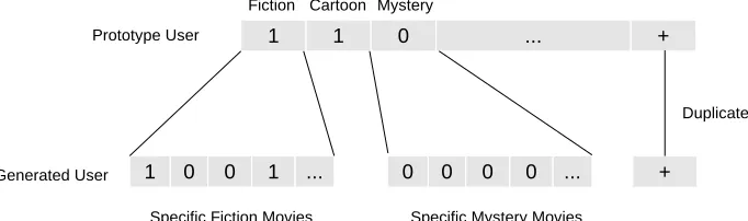
4.4 The user-movie example of Uniform Dilution. Each data entry is either 1

(watched) or 0 (not-watched). The label is a binary-valued user feature, such

as the gender. For illustration purpose, we here use different genres (i.e., Fic-tion,Cartoon) to denote non-overlapping attribute categories. But in practice,

attribute categories are mostly implicit. . . 41

4.5 Learning curves of Bernoulli-trial expansion with fixedmand different s. To ensure that we get smooth and stable learning curves, all our experiments on

synthetic data uses sampling sizes ofl = 2i,_i _{∈ {}₈,₈.₂₅,₈.₅,₈.₇₅, . . ._}_.

More-over, data sampling and 5-fold cross validation is exhaustively repeated 50

times for each value ofl. Observation: higher sparsity leads to slower

con-vergence and lower AUC upper bound. . . 45

4.6 Learning curves of Bernoulli-trial expansion with fixed sand differentm. Ob-servation: more attributes leads to higher AUC upper bound. . . 46

4.7 Learning curves of just-1 expansion with different expansion ratet. The num-ber of attributes and sparsity are not displayed in the legend of the figures, but

can be computed easily from Eq. (4.7). Observation: larger t leads to lower

convergence rate; however, different t does not change the AUC upper bound. . 47

4.8 Comparison of the learning curves on real datasets (the thick lines) and the

generated data. Observation: the learning curve behavior is similar for real

data and synthetic data. . . 51

4.9 The AUC learning curves of the real data (the thick black line) and synthetic

data generated by GPMF with different sparsity. Observation: higher s leads to lower upper bound. . . 53

4.10 The decision flowchart of our practical guideline. . . 59

5.1 A graphical illustration of Uniform Missing (upper figure) and Uniform

Dilu-tion (lower figure). 0 denotes missing. . . 67

5.2 Classification accuracy onreal-worlddata with different missing data mecha-nisms. For UM and UD, sparsity rate increases withsandt, respectively. Solid

and dashed lines indicate training and testing accuracies, respectively. . . 70

(11)

5.3 Linear SVM classification accuracy on synthetic large sparse data generated

from BTE with fixed expansion ratet and various missing likelihood s. Solid

and dashed lines indicate training and testing accuracies, respectively. The

rate of convergence can be measured by the training size needed to approach

convergence. . . 72

5.4 Linear SVM classification accuracy on synthetic large sparse data generated

from BTE with fixed missing likelihoods and various expansion ratet. Solid

and dashed lines indicate training and testing accuracies, respectively. The

rate of convergence can be measured by the training size needed to approach

convergence. . . 73

5.5 Linear SVM classification accuracy on synthetic large sparse data with UM

missing mechanism. Solid and dashed lines indicate training and testing

accu-racies, respectively. The rate of convergence can be measured by the training

size needed to approach convergence. . . 74

5.6 Linear SVM classification accuracy on synthetic large sparse data with JE

miss-ing mechanism. Solid and dashed lines indicate trainmiss-ing and testmiss-ing accuracies,

respectively. The rate of convergence can be measured by the training size

needed to approach convergence. . . 75

5.7 The road map of our theoretic study about asymptotic risk. . . 77

5.8 The decision flowchart of our practical guideline. . . 84

6.1 A graphical illustration of the clustering-based feature mapping strategy. ∗

denotes missing. We set the value of each cluster-level feature as the mean of

its member features. . . 96

(12)

List of Tables

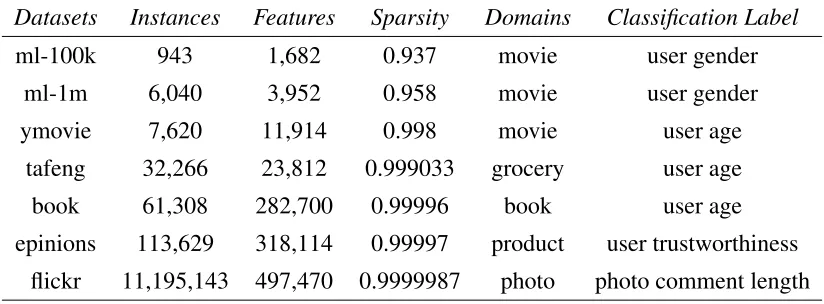
1.1 Several real-world large sparse datasets. InstancesandFeaturescorrespond to

the number of users and items in a dataset, respectively. Sparsityis calculated

as the percentage of unobserved values in each dataset. . . 3

4.1 Prototype datasets used for expansion . . . 43

4.2 Datasets for GPMFexperiment. Numbers in the parentheses are the biases added

to the posterior mean ofz. . . 52

4.3 upper bound (U) and convergence rate (V) of AUC learning curves . . . 58

5.1 Asymptotic risk ( ˆR) and convergence rate (V) of discriminative linear

classifi-cation. . . 83

6.1 Best test performance with different γ values. Each dataset is split as 4:1 for training and testing. The last column indicates the percentage of

hyper-parameters for which Algorithm 3 solved the Kernel SDCA [82] optimization

problem. . . 93

6.2 Testing accuracy on different large sparse data. Each dataset is split as 6:1:3 for training, validation and testing. The best accuracy is inboldwhile the

sec-ond best is marked with *. Underlinedresults indicate significantly better than

linear classification under McNemar’s test (p = 0.05). We have not evaluated KARMA on datasets with more than 105_{instances, because it is too expensive}

to store the kernel matrix. . . 98

6.3 Memory consumption (inmillionsof nonzero data entries) on the large datasets.

For KARMA, we need to store the kernel matrices. For other methods, we only

need to store the non-zeroes in the feature (mapping) vectors. . . 99

6.4 Training time in seconds (including feature mapping computation). The

pro-posed methods can handle theflickr-alldataset (more than 107_{instances) within}

several hours of training. . . 99

(13)

List of Appendices

Appendix A Proofs of Theorems . . . 113

(14)

Acronyms

AdaGrad Adaptive Gradient algorithm. 13, 14

AUC Area Under the receiver operating characteristic Curve. ix, x, xii, 4, 34–37, 39, 43–48,

50, 52–61, 64, 81, 86, 102

BNB Bernoulli Na¨ıve Bayes. 16

BTE Bernoulli-trial Expansion. vi, xi, 42–46, 48, 49, 52, 54, 57–59, 61, 68, 72, 73, 76–79,

81, 83–85

ERM Empirical Risk Minimization. 11, 13, 85

GNB Gaussian Na¨ıve Bayes. 16

JE Just-1 Expansion. vi, xi, 42–44, 47–49, 52, 54, 57–59, 61, 68, 75–78, 80, 81, 83–85

KARMA Kernelized Algorithm for Risk-minimization with Missing Attributes. xii, 5–8, 87–

89, 91, 93, 94, 97–100, 102

MAR Missing At Random. 40, 41, 43, 49, 66, 90

MCAR Missing Completely At Random. 23, 40, 90

MNAR Missing Not At Random. 40, 61, 90

MNB Multinomial Na¨ıve Bayes. 16

PAC Probably Approximately Correct. 7, 18–20, 27, 32, 33, 58, 83, 101

pdf prodability density function. 21

PMF Probabilistic Matrix Factorization. vi, 19–21, 23, 49, 50, 52, 56, 61, 68, 69, 71, 72

(15)

SDCA Stochastic Dual Coordinate Ascent. xii, 13–15, 93, 94, 97, 99

SGD Stochastic Gradient Descent. 13, 14

SIBM Stochastic Inference method for Binary Matrices. 21–23

SRM Structural Risk Minimization. 13

SVM Support Vector Machine. v, xi, 4, 9, 10, 12, 13, 15, 17–20, 22, 24, 26–28, 30, 32–34,

63, 64, 67, 69, 72–76, 85, 87, 88, 95, 101

UD Uniform Dilution. x, 40–43, 64, 68–70, 72, 76

UM Uniform Missing. x, xi, 23, 64, 66–70, 74, 76–78, 81–85

VC-dimension Vapnik-Chervonenkis dimension. 11, 19, 32, 65, 83

(16)

Chapter 1 Introduction

Large and sparse datasets are prevalent in the big data era. Specifically, with the rapid

emer-gence of online services and digital devices, tons of data that track our selections, usages and

feedback are generated and stored. Meanwhile, as more items are being digitized, these user

behavior datasets become sparser and sparser. For example, the famous Netflix dataset [3]

con-tains 100,480,507 ratings given by 480,189 users to 17,770 movies, where 98.822% of the

rating values are missing. Apart from rating datasets, there are many more examples of large

sparse data such as ourlikes on posts, photos and videos; our purchases on online shopping

website; our clicks on webpages or advertisements, and so forth.

Throughout this thesis, we use data sparsity to denote the percentage of missing or

un-observed values in a dataset. For a given dataset, its missing patterncan be represented by a

binary matrix where each entry indicates missing (0) or not (1). Figure 1.1 uses a toy dataset

to illustrate these different concepts. For the purpose of data modeling, we often assume that there exists a certainmissing data mechanismthat causes the missing pattern. For example, a

simple missing data mechanism is that all data points are missing completely at random. We

will further discuss different missing data mechanisms in later chapters.

It is no surprise that many datasets have such a high sparsity. With the huge number of items

in a website, each user can only consume a small portion of them. Table 1.1 gives the number of

users, items and data sparsity of several publicly-available datasets. Specifically, the movielens

datasets1 ₍_{ml-1m, ml-100k}_{) and the yahoo-movies dataset}2 ₍_ymovie_{) contain large sparse user}

ratings on a large number of movies. Meanwhile, thetafengdataset3contains shopping records

of a large number of users on the grocery products; thebookdataset [93] is about user ratings

1_http:_//_{grouplens.org}_/_datasets_/_movielens_/

2_http:_//_{webscope.sandbox.yahoo.com}_/_{catalog.php?datatype}₌_r 3_http:_//_{recsyswiki.com}_/_wiki_/_{Grocery shopping datasets}

(17)

2 Chapter1. Introduction

Figure 1.1: A toy dataset of four instances {x1,x2,x3,x4}and 4 features{a1,a2,a3,a4}. From

left to right: the full dataset in hindsight; the actually observed dataset with 12 missing values

(sparsitys=75%); and its missing pattern.

on books collected from thebookcrossing.comwebsite; the epinions dataset [65] is about user

ratings on various types of products collected fromepinions.com. Finally, the flickr dataset [8]

contains information about whether a user haslikeda certain photo inflickr.com.

Classification is one of the most fundamental data analysis technique and is of great

impor-tance in mining and making use of the large sparse data. For example, a company may need

to classify the profitability of a product/service based on sparse user feedback vectors. For the public datasets shown in Table 1.1, various types of data labels (shown in the last column) are

also provided for building interesting and useful classifiers. Besides, in the literature, much

previous work has demonstrated that sparse data are highly useful for predictive modeling. For

example, Brian et al. [14] have demonstrated that classifying user web browsing data, which is

high-dimensional and sparse, is an effective solution for online display advertising. Kosinski et al. [50] have used thelikesin Facebook, which are sparse atomic behavioral data, to accurately

predict the personality trait of each person. The same type of data have also been used in De

Cnudde et al. [15] for improving micro-finance credit scoring. Meanwhile, large and sparse

fine-grained transactional (invoicing) data have been used in Junqu´e de Fortuny et al. [41] to

build effective linear classification models for corporate residence fraud detection. Mcmahan et al. [63] have demonstrated how extremely sparse data and linear classification can solve the

advertisement click prediction tasks in the industry. Martens et al. [61] have used massive,

sparse consumer payments data to build linear predictive models for targeted marketing.

All these prior works rely heavily on linear models in classifying large sparse data. The

most important reason for doing this is efficiency: the time complexity of linear classifiers scale

linearly with the number of non-missing values. This would be especially important because

the sample size and feature dimension of these data could be extremely large, while predictions

(18)

1.1. ResearchQuestions 3

Table 1.1: Several real-world large sparse datasets. InstancesandFeaturescorrespond to the

number of users and items in a dataset, respectively. Sparsityis calculated as the percentage of

unobserved values in each dataset.

Datasets Instances Features Sparsity Domains Classification Label

ml-100k 943 1,682 0.937 movie user gender

ml-1m 6,040 3,952 0.958 movie user gender

ymovie 7,620 11,914 0.998 movie user age

tafeng 32,266 23,812 0.999033 grocery user age

book 61,308 282,700 0.99996 book user age

epinions 113,629 318,114 0.99997 product user trustworthiness

flickr 11,195,143 497,470 0.9999987 photo photo comment length

vectors tend to be linearly separable, which makes linear modeling effective for classifying

such data. As a result, linear classification is still an essential tool for mining large sparse data

in practice.

However, despite its scalability, a linear classifier is not always optimal in terms of

clas-sification accuracy. Notice that linear classifiers have assumed that the input vectorxand the

predicted value f(x) is of a linear relationship, i.e., f(x)=w·x. As a result, they cannot learn

complex data structures. In recent years, the success of matrix factorization algorithms in many

collaborative filtering applications have verified the assumption that large sparse data tend to

be low-rank, which cannot be fitted by a linear model. The low rank assumption also has a

nice intuition as items/users can often be well-described by a relatively small number of la-tent factors. Obviously, the major challenge of applying non-linear models on large datasets is

scalability. In this thesis, we will also try to address how to learn the non-linear data structures

such as low-rankness, in a more scalable manner.

1.1 Research Questions

In order to classify large sparse data more effectively, several important questions need to be answered. The first question is about how data sparsity would affect classification performance:

(1). How different properties of a dataset, such as the sparsity rate, the mechanism of

missing data systematically affect convergence behavior of classification?

Theoretically, a classifier’s generalization ability improves as it learns from more and more

(19)

a given hypothesis class. To visualize this theoretical result, in Figure 1.2, we conduct several

classification experiments on large sparse datasets as an example. We train linear Support

Vector Machine (SVM) using 5-fold cross validation with larger and larger sample size. As can

be seen in the figures, both AUC (Area Under the receiver operating characteristic Curve) [22]

and accuracy (0/1 loss) keep increasing until the entire datasets are used. Meanwhile, from the

curves of the largest dataset we have (flickr), we could see the trend that AUC/accuracy starts to converge.

flickr epinions

book ymovie

log₂(N)

Figure 1.2: Learning curves of several real-world datasets measured by 5-fold cross-validation

accuracy and AUC. All data samplings are repeated for 5 times, the regularization parameter

of the SVM is tuned using a held-out dataset on the grid [2−10,2−9, . . . ,210].

If we want to further improve classification performance, Figure 1.2 implies that collecting

more data instances is almost always beneficial for these large sparse datasets. The same result

has also been observed in the experiments performed by Junqu´e de Fortuny et al. [40], which

suggest thatbigger data is indeed better.

(20)

1.2. Challenges andOurApproach 5

amount of data needed for getting a certain accuracy/AUC, we need to know how fast a learn-ing curve converges and its converged value (asymptote). In this paper, we denote these two

properties as the convergence rate and the asymptotic performance of learning, respectively.

They are also basic problems in the Statistical Learning Theory [88], which have been

exten-sively studied. Unfortunately, previous work has not studied how data sparsity under different missing data mechanisms would affect these two learning curve behaviors. Chapters 3-5 of this thesis will provide an in-depth study of this research question for (discriminative) linear

classifiers and na¨ıve Bayes classifier, which is a generative classifier.

Knowing the relationship between data sparsity and the learning convergence behavior of

classification is necessary to estimate the gain (in terms of accuracy) and cost (in terms of data

collection) of a sparse data classification task. Meanwhile, when a (large and sparse) dataset

is given, it is important to have a classifier that can get better accuracy in a scalable manner.

Though the popular linear classifiers are very efficient, they can hardly learn the non-linear structures in the data, hence accuracy may suffer. This motivates us to study the following research question:

(2). How to efficiently learn non-linear data structures when classifying large sparse data?

It is acknowledged that linear models do not have a rich learning capacity. As a result, they

could hardly fit the complex structures in a dataset which in turn harms classification accuracy.

In recent years, the field of collaborative filtering has witnessed the success of various low-rank

methods in learning large sparse data, which implies that large sparse data tend to have latent

structures that are non-linear (e.g., the low rank structure).

However, the biggest obstacle for applying non-linear models to large datasets is

scalabil-ity. In fact, the very high feature dimensionality makes it hard to apply deep neural network

methods; meanwhile, the large sample size also makes kernel machines intractable. Apart

from scalability, another challenge is to find an appropriate non-linear model that can learn

data low-rankness during classification. In this thesis, we will focus on the KARMA

(Kernel-ized Algorithm for Risk-minimization with Missing Attributes) kernel proposed in [29], which

has theoretical guarantee in learning low-rank structures in the sparse data. We investigate

strategies to scale up the method for handling very large datasets.

1.2 Challenges and Our Approach

(21)

1.2.1 Large sparse data and learning convergence behavior

There is no universal answer for how data sparsity would affect learning convergence behavior. It depends on themissing data mechanismthat causes data sparsity. Unfortunately, for a

real-world sparse dataset, the actual mechanism that causes sparsity is usually complicated. For

example, a missing movie rating does not necessarily mean that the user has not watched the

movie. Some users may prefer to rate movies that they like, some may rate those they dislike

while some may prefer to rate when (s)he disagrees with the current average rating. The

miss-ing pattern of a real-world large sparse dataset is a complex mixture of many different factors. To control this complexity, in this thesis, we consider several basic missing data mechanisms

that are common for large sparse data in general.

Another challenge is how to empirically study the learning behaviors, especially the

conver-gence behavior of classifying large sparse data. As can be seen in Figure 1.2, publicly available

real-world sparse datasets are hardly large enough to reveal the convergence of classification.

In this thesis, we address this challenge by using synthetic data generation. To ensure that the

generated data are realistic, our approach is to sample data instances from the probabilistic

model of the real-world datasets. After generating synthetic datasets, which can be arbitrarily

large, we are able to systematically vary data sparsity with different missing data mechanisms

and empirically study the convergence behaviors of different classifiers.

The third challenge is how to understand and verify the observations obtained from

syn-thetic experiments. Specifically, do the observations hold consistently or do they hold only

under certain conditions? For this purpose, we study different types of missing data mecha-nisms for binary data as well as real-valued data. Besides, our study covers different popular classifiers for large sparse data, including na¨ıve Bayes and also discriminative linear

classi-fiers. For these different classifiers, we provide in-depth theoretical analyses for our

experi-ment observations based on previous results such as the Statistical Learning Theory [89] and

the convergence analysis of na¨ıve Bayes [69].

1.2.2 Large sparse data and non-linear learning

As demonstrated in previous studies on collaborative filtering tasks, low-rankness is arguably

the most significant non-linear structure that exists in many large sparse data. For

classifica-tion tasks, Hazan et al. [29] have developed the KARMA framework for learning low-rank

structures in the sparse data. Under the low-rank assumption, the framework has theoretical

(22)

sev-1.3. ThesisStructure 7

eral small to medium sized data [29]. However, the KARMA framework is hardly scalable to

large datasets because of the expensive kernel computation. In Chapter 6 of this thesis, we

in-vestigate the inner mechanism of the KARMA kernel with theoretical and empirical analyses.

We find that a KARMA kernel is not only possible but also effective (in terms of accuracy) to

be approximated using scalable feature mapping strategies. We demonstrate that the proposed

feature mappings not only significantly outperform linear classification, but also is scalable for

large and sparse datasets even on a normal desktop computer.

1.3 Thesis Structure

In this introductory chapter, we have described the problem, the motivation and the research

questions of the thesis. In Chapter 2, we describe the theoretical background of classifying

large sparse data. We introduce different types of efficient classifiers on large sparse data, including na¨ıve Bayes which is a generative classifier and discriminative linear classifiers such

as linear SVM and Logistic Regression [23]. In particular, we address the reason why these

classifiers can efficiently handle data sparsity.

In Chapter 3, we study how data sparsity could affect the convergence behavior of a linear SVM classifier. We propose a novel approach to generate large sparse binary data from

real-world datasets, using statistical inference and the data sampling process of the PAC (Probably

Approximately Correct) framework [89]. We then study the convergence behavior of linear

SVM with synthetic experiments, and make several important observations. We also offer theoretical proofs for our observations by studying the Bayes risk and PAC bound. These

experimental and theoretical results are valuable for learning large sparse datasets with linear

SVM.

In Chapter 4, we extend our study to na¨ıve Bayes classifier which is a simple generative

model widely used on large sparse data because of its efficiency. For na¨ıve Bayes, we study how different mechanisms of missing data, data sparsity and the number of attributes systematically affect its learning curves and convergence. We consider several common missing data mech-anisms and propose novel data generation methods based on these mechmech-anisms. We generate

large and sparse data systematically, and study the entire AUC learning curve and convergence

behavior of na¨ıve Bayes. We not only have several important observations, but also provide

detailed theoretical studies. Finally, we summarize the results as a guideline for classifying

large sparse data in practice.

(23)

discrim-8 Chapter1. Introduction

inative linear classifiers. While the previous chapters only consider missing data mechanisms

and synthetic generations of binary data, we now generalize them to real-valued datasets. Using

synthetic experiments, we observe several important learning curve behaviors under different missing data mechanisms. We derive several lemmas which prove that our observations

con-sistently hold for different linear classifiers and different loss measures. Practically, our studies help to determine if or when obtaining more data and/or obtaining missing values in the data is worthwhile or not. This can be very valuable in many applications.

In Chapter 6, we study how to efficiently learn non-linear structures when classifying large sparse datasets. Many studies suggest that large sparse data often have a low-rank structure.

By finding the polynomial approximation to the low-rank space, Hazan et al. [29] developed

a kernel algorithm (KARMA) for classifying such datasets with a higher accuracy. In Chapter

6, we develop novel scalable feature mappings to efficiently approximate the kernels used in KARMA. In experiments, our method is comparable with KARMA on medium-sized data and

scales well to larger datasets that KARMA does not. Our method also significantly outperforms

linear classifiers on datasets of various sizes.

(24)

Chapter 2 Background

In this chapter, we introduce the basic settings of a standard classification task. We distinguish

the definitions of a generative classifier and a discriminative classifier. In the second part of

this chapter, we introduce the basic learning convergence behavior of these classifiers following

the Statistical Learning Theory [89]. Finally, we give some concrete examples of classification

algorithms which will be used in later chapters, including linear SVM, logistic regression and

na¨ıve Bayes. We not only describe their problem formulations and solutions but also illustrate

their efficiency in dealing with sparse data.

2.1 Classification

The general purpose of a classification algorithm is to map a given inputxto its outputy, where

yis the target of interest. Formally, let us assume that the data space of inputxisX= _Rd_{, and}

the space of the target variable (label) isY ={1,2, . . . ,C}(while for regression task the domain ofYis continuous), whereCis the number of classes anddis the number of input features. The

data are assumed to be i.i.d. (individually independently distributed) according to distribution

D=de f p(x,y) over space{X × Y}.

For learning, the classifier is given a set of training data Strain = {x(i),y(i)}i=1,...,N which are

also distributed according toD. The goal of classification is to find adecision function f using

the training data, such that for an unseen input x, f(x) can provide a good prediction of its

unknown labely, where (x,y) is also fromD. Based on how the decision function f is learned,

we can divide classifiers intodiscriminativeclassifiers andgenerativeclassifiers.

Discriminative Classifiers. A discriminative classifier tries to either directly learn p(y|x)

(without learningp(x|y) andp(y), e.g., Logistic Regression [23]) or to directly find the mapping

(25)

10 Chapter2. Background

f (such as SVM) from a predefined class of functionsH.

Following the Statistical Learning Framework [89], a discriminative classifier will target a

non-negative loss function L f(x),y _∈

R+, which quantifies the penalty if the true target for

x isy, while the predicted target is f(x). The goal of the training process is to minimize the

following quantity, which is denoted as thegeneralization risk(true risk) of classification

RD(f)=E(x,y)∼D

h

L f(x),yi= Z

X×Y

L f(x),y

d p(x,y). (2.1)

The optimal function will be

fDiscriminative= arg min

f∈H

RD(f) , (2.2)

which can then be used for predicting unseen data in the future. When the class of functions

H is rich enough to contain all possible mappings,H = {f :X → Y}, the optimal fDiscriminative

will be equivalent to theBayes classifierwhich knows everything about the distribution p(y|x):

fBayes =arg min

f:X→Y

RD(f) (2.3)

fBayes(x)=arg min

y0

p(y0|x)L y0,y,

(2.4)

and the risk incurred by the Bayes classifier is denoted as theBayes risk:

RBayes_D (f)= E(x,y)∼D

h

L fBayes(x),yi.

(2.5)

It is obvious that the Bayes risk is the smallest risk a classifier can get given D, even in an

idealistic setting.

Generative Classifiers. Unlike a discriminative classifier, a generative classifier tries to

estimate p(x|y) and p(y) by assuming a certain probabilistic model Mfor the data. The model

M is a prior belief of what p(x|y) and p(y) should be like, which in turn allows the classifier

to estimate the two distributions, ˆp(x|y,M) and ˆp(y), from the given data. Afterwards, the

classifier uses the Bayes rule to find the estimation of p(y|x) :

p(y|x)≈ pˆ(y|x,M)= pˆ(x|y,M) ˆp(y) ˆ

p(x) . (2.6)

Finally, it acts the same as a Bayes classifier (Eq. (2.4)) in learning f, except it uses the

estimated distribution rather than the true distribution:

fGenerative = arg max

y

ˆ

(26)

2.2. Convergence ofDiscriminativeClassifiers 11

as the learned mapping.

Ng and Jordan [69] have provided detailed discussion of the advantages and disadvantages

of discriminative and generative classifiers. However, this is not the focus of this thesis. In the

previous chapter, we have demonstrated how linear classifiers behave as we increase the size

of large sparse data (Figure 1.2). Here we introduce the theoretical background behind this

phenomenon, i.e., the convergence of classification.

2.2 Convergence of Discriminative Classifiers

As described earlier, since only the training dataS_trainare given, a discriminative classifier will

use theEmpirical Risk

Remp_S

train∼D(f)=

1

N N X

i=0

L f(x(i)),y(i)

(2.8)

to estimate the generalization risk in Equation (2.1). A most simple discriminative classifier

will use the ERM (Empirical Risk Minimization) principle [89] for training1. In other words,

it finds the decision function by

f_S∗

train :=arg min

f∈H

n Remp_S

train∼D(f)

o

. (2.9)

Because of the Uniform Convergence of ERM [88], whenNbecomes sufficiently large, the empirical risk, f_S∗

train will converge to the optimal generalization (true) risk:

Remp_S

train∼D(f

∗

Strain)→

p

N→∞min

f∈H

RD(f) := RˆD, (2.10)

Here the symbol→_Np_→∞represents theconvergence in probabilitywhenN → ∞, which follows

the definition in Vapnik et al. [88]. We denote theasymptotic riskas ˆRD. Notice that the above

results hold so long as H has bounded complexity (VC-dimension [88]), which is true for

discriminativelinear classifiers:

H_linear ={f|f(x)=w·x,w∈_Rd}. (2.11)

As we increase training size, N, the convergence rateof learning describes how fast the

empirical risk converges to the asymptotic risk ˆRD. For illustration purpose, Figure 2.1 gives

the convergence behavior of empirical risk and true risk of the discriminative training process.

(27)

Figure 2.1: As the training size Nincreases, the empirical risk (Remp_S

train∼D) and true risk (RD) of

a classifier f_S∗

train will converge.

2.3 Convergence of Generative Classifiers

The learning convergence behavior of a generative classifier is similar to that of a discriminative

classifier. Basically, the learning process converges because of the convergence of the estimated

probabilities to their true values. In other words, the optimal classifier fGenerative(x) computed

by:

fGenerative(x)=arg max

y

ˆ

p(y|x,M)= arg max

y

ˆ

p(x|y,M) ˆp(y) (2.12)

converges because of the convergence of ˆp(x|y,M) and ˆp(y) to their corresponding asymptotes.

Finally, if we quantify the predictive performance using the risk of classification in Equation

(2.1), we expect a very similar convergence curve as the discriminative classifiers.

In the next subsection, we describe concrete examples of discriminative and generative

classifiers, which will be used in the thesis.

2.4 Discriminative Linear Classifiers

Because of their efficiency in dealing with large datasets, we focus on discriminative linear classifiers, including linear SVM and Logistic Regression. A practical algorithm for

discrimi-native classification often optimizes an objective function of the form

min

f∈HR

emp

(28)

2.4. DiscriminativeLinearClassifiers 13

whereC(f) quantifies the complexity of the function f andλis the parameter that controls the

strength of regularization. This strategy (adding regularization to ERM principle) is known as

the Structural Risk Minimization (SRM) principle [89], which is especially necessary when the

sample size is small.

Without loss of generality, consider the binary classification problem whereYhas only two

distinct elements {+1,−1}. Both linear SVM and Logistic Regression consider the following objective function:

min

w∈Rd

1

N N X

i=1

L(f(x(i)),y(i))+ λ 2||w||

2_,

(2.14)

where f(x) = wT_x_{is the decision function whose sign can be used for prediction. For linear}

SVM, we set the loss function as:

Lhinge(f,y)=max{0,1−y f}, (2.15)

which is known as thehinge loss, while for logistic regression, we use thelogistic loss:

Llogistic(f,y)=ln(1+e

−y f

). (2.16)

There are many other loss functions for linear prediction, such as squared loss Lsquared(f,y) =

(y− f)2, and squared hinge loss Lsquared-hinge(f,y) = (max{0,1−y f})2. These commonly used

loss functions are actually convex surrogates [2] of the error rate(0-1 loss), which is defined

asL0-1(f,y)= I(sign(f),y), whereI(A) equals 1 if eventAis true and 0 otherwise..

There are many algorithms and their corresponding software packages that can solve

Equa-tion (2.14). TradiEqua-tional methods use the quadratic programming algorithms which cannot scale

well to large scale learning problems. Recently, efficient solvers have been proposed using SGD (Stochastic Gradient Descent) [81, 19] or coordinate ascent [34, 82], which work on the

primal and dual problem of Eq. (2.14), respectively. To illustrate the efficiency of these modern solvers on learning sparse data, we briefly review the AdaGrad (Adaptive Gradient algorithm)

[19] and the SDCA (Stochastic Coordinate Dual Ascent) [82] algorithm as representatives of

each family of optimizers.

AdaGrad Let us consider the standard SGD algorithm. At iterationt, SGD randomly chooses

a data instance (x(t),_y(t)_{) to observe, then updates the model parameter of (2.14) by}

wt+1 =wt −ηt ∂ht ∂wt

(29)

whereηtis the learning rate andht = L(f(x(t)),y(t))+λ₂||w||2is the regularized loss for the current

instance. With a good step-size strategy forηt, ft can converge to the optimal linear function

with ˜O(1/t) convergence rate.

Compared to other SGD variants, AdaGrad [19] is the most suitable solver for learning

sparse data. The most important design of AdaGrad is to update each attribute with diff er-ent learning rates to adapt for their different sparsity rates. Unlike Equation (2.17), AdaGrad updates using:

wt+1 =wt−ηtG

−1/2

t ∂ht ∂wt , (2.18) where Gt = t X

τ=1

∂hτ ∂wτ(

∂hτ ∂wτ)

T

(2.19)

is ad×dmatrix whose diagonal elements are the sums of squared historical gradients on each

attribute. This adaptation is especially useful because sparsity rates for each attribute are often

quite different.

SDCA As its name suggests, SDCA [82] works on the dual problem of Eq. (2.14) using

stochastic coordinate ascent. If we consider Eq. (2.14) as the primal problem:

min

w∈Rd

P(w), whereP(w)= 1

N N X

i=1

L(f(x(i)),y(i))+ λ 2||w||

2

(2.20)

its dual can be formulated as:

max

α∈RN

D(α), whereD(α)= 1

N N X

i=1

−φ∗_i(−α(i))− λ

2|| 1

Nλ N X

i=1

α(i)_x(i)_||2 _(2.21)

αis the N-dimensional dual coefficient andφ∗_i(·) is the convex conjugate ofL(·), see [83] for detail.

The duality theory implies that the gap between the primal and dual objectives are always

non-negative:

∆gap(α) :=P(w(α))−D(α)≥ P(w(α))−P(w∗)≥0, (2.22)

where w(α) := _Nλ1 PN i=1α(

i)_x(i)_{. This} _{duality gap} _{can be used to measure the accuracy of a}

current solutionα, w.r.t. the optimal one.

The implementation of the SDCA solver is simple. Briefly speaking, SDCA initializesαto

beα0 = 0. At each iterationt, it randomly picks an elementα(

i)

t from{α

(1)

t , α

(2)

t . . . , α

(N)

t }(with

replacement), and updatesα(ti)to beα

(i)

(30)

2.5. Na¨ıveBayesClassifier 15

the selected coordinate i. This process is repeated until the duality gap is sufficiently small, e.g.,∆gap(α)<0.001.

While this idea is quite simple, we focus more on its efficiency in dealing with highly-sparse data. The analysis in Shalev et al. [82, 83] implies that the time complexity for the

SDCA solver to achieve∆gap(αt)≤ on the logistic regression problem is

˜

O (1− s)·d

N+minnR

2

λ,

r NR2

λ

o!

(2.23)

while on the linear SVM problem is:

˜

O (1− s)·d

N+minnR

2 λ, r NR2 λ o ! , (2.24)

whereR:=maxi||xi||2measures the radius of the input. As before,srepresents the sparsity rate

(percentage of zeros) in the data. It can be seen that this algorithm has nice scalability since it

only scales linearly with the number of non-missing values (i.e., (1−s)dN).

We would like to mention that AdaGrad and SDCA have similar optimization speed

ac-cording to our empirical results on classifying large sparse data. In our later experiments, we

extensively use SDCA as the optimizer for discriminative linear classifiers on large sparse data.

2.5 Na¨ıve Bayes Classifier

Na¨ıve Bayes makes assumptions about the generation process and the underlying distribution

of the observed data. This is different from the discriminative classifiers described above, which have adopted adistribution freeapproach.

Specifically, the Na¨ıve Bayes model assumes that the data distribution of each feature xjis

independent of one another, when its labelyis given. In other words, the conditional probability

p(x|y) can be factorized as:

p(x|y)=

d Y

j=1

p(xj|y). (2.25)

Finally, a classification decision is made by

fNB(x)= arg max

y

p(y)p(x|y)= arg max

y

p(y)

d Y

j=1

p(xj|y). (2.26)

The training process of a na¨ıve Bayes classifier is basically to estimate all the probability

(31)

indepen-16 Chapter2. Background

dence assumption greatly simplifies density estimation, especially when the number of

dimen-siondis high: it reduces the density estimation of the joint distributionp(x|y) to the estimation

of a collection of univariate probabilities.

In practice, there are different prior models for estimating the density of p(xj|y) for different

types of data. For example, when xj ∈ R is a continuous variable, p(xj|y) is often estimated

using a one-dimensional Gaussian prior:

p(xj|y)∼ N(µj,y, σ2j,y), (2.27)

where parametersµj,yandσ2_j,yare computed using maximum likelihood estimation. This model

is denoted as Gaussian Na¨ıve Bayes (GNB) classifier.

In situations like text classification, a feature value xj may represent a discrete value. For

example, whether each word of the vocabulary appears in a document (binary) or its frequency

of appearance (ordinal). In this case, p(xj|y) can be modeled using either a multinomial

dis-tribution or a multivariate Bernoulli disdis-tribution, which leads to the Multinomial Na¨ıve Bayes

(MNB) and Bernoulli Na¨ıve Bayes (BNB) classifier, respectively. One of the major difference between the two models is that BNB only considers the binary state of whether each event

occurs while MNB also models the frequency of appearance. In practice, both BNB and MNB

are highly effective for classifying sparse data such as text documents, though each model has its own preferred setting [62].

We would like to mention that MNB is also a linear classifier in the sense that the decision

function can be represented as a linear combination of the input feature values; see Rennie et

al. [75] for the detailed derivation. Meanwhile, BNB is not a linear classifier. In Chapter 4, we

will study BNB and its convergence behavior on large sparse data.

For handling sparse data, a Gaussian Na¨ıve Bayes model can simply ignore the features

with missing values in computing the decision function in Eq. (2.26). Meanwhile, both MNB

and BNB can naturally model the missing features because both Multinomial and Bernoulli

distribution can model the absence of an event. Moreover, the time complexity of a na¨ıve

Bayes classifier scales linearly with the number of non-missing values only. Take BNB as

an example, estimating the marginal probability p(xj|y) amounts to counting the number of

non-missings in feature xj and classy.

2.6 Conclusion

In this chapter, we have introduced the general setting of a classification task. Moreover, we

(32)

2.6. Conclusion 17

principles. To illustrate the key issues of large-scale classification, we also reviewed the

theo-ries of learning convergence behavior for different types of classifiers. Finally, we use concrete algorithms of discriminative linear classifiers and na¨ıve Bayes classifiers to illustrate how these

classifiers handle large sparse data and achieve fast learning.

Starting from the next chapter, we present the major contributions of the thesis, i.e.,

analyz-ing how data sparsity would affect the convergence behavior of a classifier. Our study covers both discriminative linear classifiers such as linear SVM and also generative classifier such as

(33)

Chapter 3 Data Sparsity in Linear SVM

Large sparse datasets are common in many real-world applications. Linear SVM has been

shown to be very efficient for classifying such datasets. However, it is still unknown how data sparsity1would affect its convergence behavior. To study this problem in a systematic manner, we propose a novel approach to generate large and sparse data from real-world datasets, using

statistical inference and the data sampling process of the PAC framework [89]. We first study

the convergence behavior of linear SVM experimentally, and make several observations, useful

for real-world applications. We then offer theoretical proofs for our observations by studying

the Bayes risk and PAC bound. Our experiment and theoretical results are valuable for learning

large sparse datasets with linear SVM.

3.1 Introduction

As described earlier, large sparse datasets are common in many real-world applications. Linear

SVM solvers such as Pegasos [81] and LibLinear [21] are popular choices to classify large

sparse datasets efficiently, because they scale linearly with the number of non-missing values. Nowadays, it is possible to train linear SVM on very large datasets. Theoretically, it is known

that larger training data will lead to lower generalization error, and asymptotically it will

con-verge to the lowest error that can be achieved [88]. However, it is still hard to answer the

following important questions about linear SVM and data sparsity:

(1). If we put in effort to reduce data sparsity, would it decrease the asymptotic generaliza-tion error of linear SVM?

1_{In our published manuscript of this chapter [54], we use the term}_sparseness_{. However,}_sparsity_and

sparse-nessrefer to the same concept. For consistency, we use data sparsity throughout this thesis

(34)

3.1. Introduction 19

(2). Would data sparsity affect the amount of training data needed to approach the asymp-totic generalization error of linear SVM?

These questions essentially concern the convergence behavior of learning, which has been

addressed in previous works. In Statistical Learning Theory [88], PAC bound gives a

high-probability guarantee on the convergence between training and generalization error. Once

the VC-dimension of the problem is known, PAC bound can predict the amount of training

instances needed to approach the asymptotic error. Barlett et al. [1] have shown that the

VC-dimension of linear SVM is closely related to the hyperplane margin over the data space. As

an initial step of understanding the impact of data sparsity on the margin of hyperplanes, Long

and Servedio [57] have given bounds for integer weights of separating hyperplanes over the

k-sparse Hamming Ball spacex ∈ {0,1}m

≤k (at mostk of themattributes are non-zero). There

also exist several SVM variants that could deal with missing data [70, 9]. However, there is still

no work could explicitly predict the convergence behavior of linear SVM when data is highly

sparse.

In this chapter, we will answer this question by systematic experiments and then verify

our findings through theoretical study. We propose a novel approach to generate large and

sparse synthetic data from world datasets. First, we infer the statistical distribution of

real-world movie rating datasets using a recent Probabilistic Matrix Factorization (PMF) inference

algorithm [32]. From the inferred distribution, we then sample a large number of data instances

following the PAC framework, so we can study the generalization error with various training

sizes.

In order to study the effect of data sparsity, we consider a simple missing data model, which allows us to systematically vary the degree of data sparsity and compare the learning

curves of linear SVM. To follow the PAC framework, we study the curves of training and

testing error rates as we keep increasing the training size. We have made several important

observations about how data sparsity would affect the asymptotic generalization error and the rate of convergence when using linear SVM; see Section 3.3.

We then analyze our observations with a detailed theoretical study. For asymptotic

gen-eralization error, we study the change of Bayes risk as we vary data sparsity. With proper

assumptions, we have proved that higher sparsity will increase the Bayes risk of the data, see

Section 3.4.1. For the asymptotic rate of convergence, we observe that different sparsity would

not change the amount of training data needed to approach convergence. We study its

theoret-ical rationale using the PAC bound, see Section 3.4.2.

(35)

20 Chapter3. DataSparsity inLinearSVM

indicate that sparser data would generally increase the asymptotic error, which encourages

practitioners to put effort in reducing data sparsity. Secondly, our results also imply that sparser data will not lead to slower learning curve convergence when using linear SVM, although the

asymptotic generalization error rate would increase.

The rest of the chapter is organized as follows. Section 3.2 gives details of our data

gener-ation approach. Section 3.3 describes our experiment and observgener-ations. Section 3.4 provides

mathematical proofs for our observations. Section 3.5 concludes the chapter.

3.2 A Novel Approach to Generate Sparse Data

To systematically study the impact of data sparsity on linear SVM, in this section, we first

propose a novel approach to generate sparse data.

3.2.1 Basic Settings

To simplify the problem setting, we only consider binary attribute values x ∈ {0,1}m and

bi-nary label y ∈ {+,−}. Our data generation approach follows the standard setting of the PAC framework [88], which assumes that data (x,y) are independently sampled from a fixed

dis-tribution P(x,y) = P(y)P(x|y). In addition, our approach uses the distribution inferred from

real-world datasets, so the generated data are realistic in a statistical sense. Specifically, we use

the datasets of recommendation systems, such as movie ratings to inferP(x,y).

Recently, datasets of recommendation systems are widely studied. They usually contain

ordinal ratings (e.g., 0 to 5) given by each user to each item. We consider each user as a data

instance and its rating on items corresponds to each attribute. To make the data binary, we only

consider the presence/absence of each rating. We choose the gender of each user as its label

y∈ {+,−}.

To infer the distribution P(x,y), we use Probabilistic Matrix Factorization [67], which is a

widely-used probabilistic modeling framework for user-item ratings data. In the next section,

we will briefly review the PMF model for binary datasets proposed by Hernandez et al. [32],

which will be used in our data generation process.

3.2.2 Review of PMF for Sparse Binary Data

ConsiderLusers andMitems, theL×Mbinary matrixXindicates whether each rating exists.

(36)

3.2. A NovelApproach toGenerateSparseData 21

predictive performance:

p(X|U,V,z)=

L Y

i=1

M Y

j=1

p(xi,j|ui,vj,z), (3.1)

where a Bernoulli likelihood is used along with the Matrix Factorization assumptionX≈U·V

to model each binary entry ofXas:

p(xi,j|ui,vj,z)= Ber

xi,j|δ(uivTj +z)

(3.2)

whereδ(·) is the logistic function

δ(x)= 1 1+exp(−x)

used to ‘squash’ a real number into the range of (0,1), Ber(·) is the pdf (prodability density

function) of a Bernoulli distribution and z is a global bias parameter in order to handle data

sparsity.

This PMF model further assumes that all latent variables are independent by using fully

factorized Gaussian priors:

p(U)=

L Y

i=1 D Y

d=1

N(ui,d|mu_i,d,vu_i,d), (3.3)

p(V)=

M Y

j=1

D Y

d=1

N(vj,d|mv_i,d,vv_i,d), (3.4)

and

p(z)= N(z|mz,vz), (3.5)

whereN(·|m,v) denotes the pdf of a Gaussian distribution with meanmand variancev. Given a

binary datasetX, the model posteriorp(U,V,z|X) could be inferred using the SIBM (Stochastic

Inference method for Binary Matrices) algorithm [32]. The posterior predictive distributions

are used for predicting each binary value inX:

p(eX|X)= Z

p(Xe|U,V,z)p(U,V,z|X)dUdVdz. (3.6)

3.2.3 The Distribution for Data Sampling

Based on the above PMF model, we next describe the distribution for sampling synthetic data.

(37)

22 Chapter3. DataSparsity inLinearSVM

p(ex,y|X)= p(y)p(ex|y,X). (3.7)

Forp(y), we simply use a balanced class prior, p(+)= p(−)=0.5. This ensures equal chances of getting positive and negative instances when sampling.

Now we describe how we get p(_ex|y,X). We first divide the real-world datasetX into the

positive labeled setX₊ and the set of negative instances, X−. We infer the model posteriors

p(U,V,z|X−) and p(U,V,z|X₊) separately using the SIBM algorithm.

Notice that these inferred models cannot be directly used to generate infinite samples:

sup-pose the number of users inX₊(andX−) isL₊(andL−), the posterior predictive (3.6) only gives

probabilities for each of theseL₊(L−) existing users. In other words, the predictive distribution

could only be used to reconstruct or predict the originalX, as did in the original paper [32].

In order to build a distribution for sampling an infinite number of synthetic users, we

em-ploy the following stochastic process: whenever we need to sample a new synthetic instance

ex, we first randomly choose a user i from theL+ (or L−) existing users, and we then sample

the synthetic instance using the posterior predictive of this user. Using this process, the pdf of

p(_ex|y,X) is actually

p(_ex|y,X)=

Ly

X

i=1

p(i|y)· Z

p(_ex|U,V,z,i)p(U,V,z|Xy)dUdVdz, (3.8)

wherey∈ {+,−}, p(i|y)= _L1

y and

p(_ex|U,V,z,i)=

M Y

j=1

p(_exi,j|ui,vj,z) (3.9)

is the likelihood for each instance (existing user) ofXy, which is equivalent to Eq. (3.1). The

(38)

3.2. A NovelApproach toGenerateSparseData 23

Algorithm 1Data Sampling from a Binary PMF model infer p(U,V,z|X−) and p(U,V,z|X₊) using SIBM;

sampleV₊,z₊fromp(U,V,z|X₊);

sampleV−,z−fromp(U,V,z|X−);

foreach new instance (ex,y)do

randomly sampleyfrom{+,−}; randomly sampleifrom{1, ...,Ly};

sampleuifrom p(U,V,z|Xy);

for jin 1...Mdo

sample_exj fromBer(_exj|δ(ui·vj,y+zy));

end for

This algorithm allows us to sample infinite instances from the fixed distribution p(ex,y|X),

to be used for generating data of various sizes. Next, we will discuss how to systematically

vary the sparsity of the sampled data.

3.2.4 Missing Data Model

We employ a simple missing data model, to add and vary data sparsity. Our missing data model

assumes that each attribute has the same probability to become 0, which follows the Missing

Completely At Random (MCAR) assumption [30].

Given the probability of missing s, the missing data model will transform an instance_ex =

(_ex1,ex2, ...,exm) tox=(x1,x2, ...,xm) following:

p(x|_ex,s)=

m Y

j=1

Ber(_exj·(1−s)). (3.10)

To ease our illustration, we hereafter call this sparsification process as Uniform Missing

(UM), and the resultant data as the sparsified data. Now if instances are originally sampled

from p(_ex|y), the distribution of the sparsified data can be computed by

p(x|y,s)=

Z

p(x|_ex,s)p(_ex|y)d_ex.

When we apply this sparsification process to data generated from Algorithm 1, we denote the

resultant distribution as p(x|y,X,s)=R p(x|_ex,s)p(_ex|y,X)dex.

Using the above missing data model, additional sparsity will be introduced uniformly to

each attribute and higher s will lead to sparser data. This enables us to vary s and study the

Classification with Large Sparse Datasets: Convergence Analysis and Scalable Algorithms

Scholarship@Western

Scholarship@Western

Classification with Large Sparse Datasets: Convergence Analysis

Classification with Large Sparse Datasets: Convergence Analysis

and Scalable Algorithms

and Scalable Algorithms

Abstract

Acknowlegements

Contents

List of Figures

List of Tables

List of Appendices

Acronyms

Chapter 1

Introduction

1.1

Research Questions

1.2

Challenges and Our Approach

1.2.1

Large sparse data and learning convergence behavior

1.2.2

Large sparse data and non-linear learning

1.3

Thesis Structure

Chapter 2

Background

2.1

Classification

2.2

Convergence of Discriminative Classifiers

2.3

Convergence of Generative Classifiers

2.4

Discriminative Linear Classifiers

2.5

Na¨ıve Bayes Classifier

2.6

Conclusion

Chapter 3

Data Sparsity in Linear SVM

3.1

Introduction

3.2

A Novel Approach to Generate Sparse Data

3.2.1

Basic Settings

3.2.2

Review of PMF for Sparse Binary Data

3.2.3

The Distribution for Data Sampling

3.2.4

Missing Data Model