do not indicate a change for some species such as pricklypear, mesquite, and granj eno.
In the present investigation, 2 chained areas were sampled. Pricklypear plant density increased, par- ticularly in class 1 plants, on both areas (Tables 1, 2). The frequency increase was slight and of little value as an indication of plant distribution. The density and frequency values show that both the control and treated areas supported uniform dense stands of pricklypear.
Chaining appears to result in the scattering of pricklypear and the establishment of many new plants (Table 1). However, as pointed out in Part II of the Soil Conservation Service report (USDA,
1964b) chaining has some value in the control of single-stemmed trees such as mesquite. Smaller brush species, such as blackbrush and condalia, bend and little damage results from chaining. If the tops are broken, profuse sprouting usually occurs.
LITERATURE CITED
ALLISON, D. V., AND C. A. RECHENTHIN. 1956. Root plow- ing proved best method of brush control in South Texas. J. Range Manage. 9:130-134.
Box, T. W. 1964. Changes in wildlife habitat composi- tion following brush control practices in South Texas. Trans. N. Amer. Wildl. and Nat. Res. Conf. 29:432-438. Box, T. W., AND J. POWELL. 1965. Brush management techniques for improved forage values in South Texas. Trans. N. Amer. Wildl. and Nat. Res. Conf. 30:285-296. DAMERON, W. H., AND H. P. SMITH. 1939. Pricklypear
eradication and control. Texas Agric. Exp. Sta. Bull. 575. 55 p.
Discussion and Development of
the Point-Centred Quarter Method
of Sampling Grassland Vegetation
A. HEYTING
Biometrician, Department of Research and Specialist Services, Ministry of Agriculture, Rhodesia.1
Highlight
The point-centered quarter method of sampling grassland vegetation is critically examined. Statistical techniques of processing data collected by the method are presented. These techniques are discussed in the light of findings from a sampling experiment at Matopos Experiment Sta- tion, Rhodesia.
Excellent methods of grassland sampling, the results of which are amenable to statistical analysis, l At present: Statistician, Statistics Dep., National Council
for Applied Research (T.N.O.), Wageningen, Holland.
DARROW, R. A. 1950. The effectiveness of 2,4,5-T on pricklypear. Research Report, Seventh Annual North Central Weed Control Conf. p. 234.
GOULD, F. W. 1962. Texas plants-a checklist and eco- logical summary. Tex. Agri. Exp. Sta. MP 585. 112 p. HAMILTON, R. D. 1950. The use of TCA to eradicate
pricklypear cactus. Research Report, Seventh Annual North Central Weed Control Conf. p. 238.
HOFFMAN, G. O., AND J. D. DODD. 1967. Herbicidal con- trol of pricklypear in the South Texas Plains. Proc. 20th Annual Southern Weed Conf. 191-198.
HUMPHREY, R. R. 1958. The desert grassland, a history of vegetational change and an analysis of causes. Bot. Rev. 24: 193-252.
INGLIS, J. M. 1964. A history of vegetation on the Rio Grande Plains. Texas Parks and Wildlife Dep. Bull. No. 45. 122 p.
JOHNSTON, M. C. 1963. Past and present grasslands of southern Texas and northeastern Mexico. Ecology 44: 456-466.
LEHMANN, V. W. 1965. Fire in the range of Attwater’s prairie chicken. Proc. Fourth Annual Tall Timbers Fire Ecology Conf. 127-143.
POWELL, J., AND T. W. Box. 1966. Brush management influences preference values of South Texas woody spe- cies for deer and cattle. J. Range Manage. 19:212-214. POWELL, J., AND T. W. Box. 1967. Mechanical control and
fertilization as brush management practices affect forage production in South Texas. J. Range Manage. 20:227- 236.
U.S.D.A. 1964a. Grassland restoration: The Texas brush problem. Unnumbered Bull. USDA Soil Cons. Serv., Temple, Texas. 17 p.
U.S.D.A. 1964b. Grassland restoration. Part II: Brush control. Unnumbered Bull. USDA Soil Cons. Serv., Temple, Texas. 39 p.
have been developed for dense vegetation and for situations where the grass is not grazed or cut. Prominent among these are the “point methods.” If the vegetation is very sparse then these methods are rather inefficient, especially if interest is cen- tered on measurements made at ground level, as may be the case when the grassland under study is being grazed by game or cattle. In such situations, distance measurement methods, such as the point- centered quarter (P.C.Q.) method, may be useful. By these methods positive information on species composition and density is obtained at all sampling positions whereas, with the point methods, most sampling points would yield no more information than that no “hit” can be recorded.
P.C.Q. SAMPLING
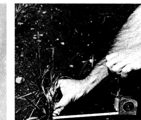
FIG. 1. The P.C.Q. calibrator.
while the pattern of vegetation distribution re- mains relatively stable. The study of pattern itself will be dealt with in a future paper. Statistical techniques for the processing of P.C.Q. data are presented and examples of their application are given.
Procedures
The below description of field procedures closely follows the directions given by Dix (1961).
Sampling points are distributed within the sampling area according to a systematic pattern. They are situated at equal intervals along parallel straight lines. Points on alternate lines are staggered. If the distance between suc- cessive points on each line is d, then the lines themselves must be a distance rhdv?? apart. This produces a lattice of points such that each point is equidistant from its six nearest neighbors. In practice these instructions need not be followed rigidly, the main aim being to get a roughly uniform distribution of sampling points. The location of points is facilitated by the use of a surveyor’s arrow and compass. Each sampling point is found by pacing a pre- determined number of steps along a compass line and then placing the arrow vertically into the ground, guided by a notch cut in the tip of the sampler’s boot.
The area around each sampling point is divided into four quarters, delineated by two lines through the sampling point, one parallel to and another perpendicular to the direction of the compass line. The demarcation of quarters is aided by filing four small marks on the surveyor’s arrow in such a way that each mark is 90” from its nearest neighbor. I have chosen the name “station” to describe a sampling point together with the four quarters around it.
Within each quarter, the distance from the sampling point (base of the surveyor’s arrow) to the nearest living herbaceous shoot (nearest point of root development for creeping species) is measured at ground level and recorded by species and by station.
Two minor departures from the above procedure are suggested. Firstly, the orientation of quarters need not be constant for all stations. Effort and time may be saved to
FIG. 2. The P.C.Q. calibrator in use.
a minor extent by placing the surveyor’s arrow without reference to the direction of the marks which demarcate the quarters, and this is recommended. Secondly, it has been found that replacing the compass line by a steel tape or by pacing between siffhting rods both work quite well in oben grassland areas. Fveryklement of choice on the part of the operator is removed if ‘predetermined positions along the tape define sampling points. This is desirable to avoid biased findings.
Instruments.-1 have developed an instrument to make the field work easier. It is called the “P.C.Q. calibrator” (Fig. 1 and 2) and is a more sophisticated version of the surveyor’s arrow. The measuring device, in this instance a tape mea- sure, is attached to the instrument in such a way that it can rotate around the central shaft. The equivalent of filing marks on the surveyor’s arrow is a dial which is attached to the shaft just above the tape measure together with an indicator hand which is fastened to the tape measure itself. The tip of the shaft holds a sharpened blade which prevents the shaft from turning after it has been inserted in the ground.
Data Recording-.-The data form of Fig. 3 has shown itself to be quite convenient for subsequent data processing.
S I T E “-‘d&~ B SAMPLING DATE /Y/2//9-4
Except for the last five columns and the last line, the form is identical to that suggested by Dix (1961).
The stations in a single sampling area are numbered con- secutively on successive data forms. The entries correspond- ing to stations and species are the recorded distances. Note that there are four such distances per station. The Xd column contains the total distance for each species. The nij columns contain the number of times a species is en- countered j times. There are, for example, three stations at which D. nemordis is encountered twice (stations 1, 8, and 9). The bottom line contains all the column totals.
Two checks have to be made. Firstly, the sum of the first 10 column totals must, of course, equal the total of the zd column. This column is, in fact, included solely to pro- vide this check. Secondly, if the sum of the nij column is denoted by nej and the number of stations on the form is denoted by n, then the following must be true:
i (jnej) = 4n
j=l
For example, from the data sheet of Fig. 3 we have:
For the entire sampling area a summary of the last four columns is made, so that nij on the summary is the total number of stations in the sample where the ith species is recorded j times. Equating n now to the total number of stations in the sample, the second check above must, of course, apply equally to this summary.
The purpose of recording the nij and the total distances per station will become clear in subsequent sections.
Vegetation Parameters
Dix (1961) defines several parameters by which to describe the vegetation.
The relative frequency of a species is the number of stations at which the species is recorded at least once, expressed as a proportion of the total num- ber of stations in the sample. The relative density of a species is that proportion of the total number of quarters in the sample where the species was recorded. Both these quantities may be expressed as percentages. The comparison between the rela- tive frequency and relative density of a species gives an indication of the manner in which the species is distributed over the sampling area. A relatively high relative frequency indicates a wide distribution of small clumps while near equality of the two implies a concentration of the species in large clumps.
The mean distance per quarter is calculated and Dix claims that its square gives the mean area per shoot. This claim is based on work done by Cottam et al. (1953) who showed that if the P.C.Q. method is applied to sample a population of randomly dispersed points then the square of the mean distance per quarter provides a close estimate of the mean area per point. Unfortunately, the application of this result to the P.C.Q. sampling of grassland will only be valid in rare instances. Grassland vegetation is usually arranged in clusters
of individual plants, each of which may consist of numerous shoots. In such cases the distribution of shoots cannot be assumed to be random and the mean area as obtained above loses its meaning. This observation is supported by statistical evi- dence, derived from data which were obtained at a sampling site at Matopos Experiment Station, Rho- desia. There the four distances which are mea- sured at a single station were found to be positively correlated, thus disproving a hypothesis of random distribution of shoots. The evidence is presented in greater detail in the next section.
Some Statistical Results
In this section capital letters will be used to indi- cate variables while their realizations are denoted by lower case letters.
Given a sampling area, a fixed sample size, n say, and a method of selecting the n sampling points, the following notations apply:
xik
pijk
Fi E(Fi)
Nij
D km
Dk.
D..
E(D .
.)v( Fi)
v(D .
.)the variable which records the number of quarters in which the ith species is en- countered at the kth station,
the probability that, for any one sample, xii, has a realization equal to j,
the relative density = ( i1&) / 4n, the expectation of Fi, also called the “true relative density” corresponding to the sam- pling method,
the variable which counts the total number of xii< in a sample which are equal to j, the variable which measures the distance in the mth quarter of the kth station of a sample,
4, the mean distance per quar- ter at the kth station,
( ilDkJ/ n, the mean distance per quar- ter over all stations,
the expectation of D . ., also called the “true mean distance per quarter” corresponding to the sampling method,
the estimate of variance of Fi and the estimate of variance of D . . .
It follows directly from the above definitions that the relative density (fi) and the mean distance per quarter (d. .), both calculated from the sample data, are unbiased estimates of the true relative density of the ith species and the true mean dis- tance per quarter respectively. The easiest way to calculate fi is as
fi =
( i
j
jnij)/4n, =IP.C.Q. SAMPLING 373
Estimation of the Variance of the Relative Density Per definition,
variance (Xik) = E[ {Xi,< - E(Xik)}2] =
On the assumptions that, for fixed i, the Xik are mutually uncorrelated and that, for fixed i and j, the pijk are constant and equal to pij say,
variance (Fi) = variance [ i (Xik)/Jn]
k=l 1
=-
[ i variance (Xik)
16n” kZl
1
’
=-El
[ jI (j”Pij>
- (
$1jPij)2] 7 and pij may be estimated by cij = nij/n. An esti- mate of variance of the relative density of the ith species may then be obtained by replacing pij in the above expression by its estimate, whence1
v(Fi) = m nil (j2nij) - ( i_inil>^] 9 which may be expanded to give
v(Fi)
=A
[nib - nil) + 4ni2(n - ni2)+ 9nis(n - nis) + 16nib(n - ni4) - 4nil niz - 6nil nis - 8nil nib
- 12ni2ni3 - 16ni2 ni4 - 24nia ni4] . Variance of the Relative Density with
Systematic Sampling
If the sampling points are randomly dispersed over the sampling area, the above assumptions are met and the variances of the relative densities may be estimated as shown. In practice, perfectly ran- dom distribution of sampling points cannot be achieved and even approximate randomization is very laborious. The method is to select at random intersections of the lines of a fine, imaginary grid which is superimposed on the sampling area. Sampling points can be located in the field by reference to a set of coordinate axes.
With systematic sampling there can be no guar- antee that the conditions of the previous section are met. If interest is confined to the specific arrangement of plants as found in the sampling area at the time of taking the sample, this will certainly not be the case. If, on the other hand, a process is hypothesized by which the vegetation pattern is generated and if interest attaches to the vegetation considered as a random realization of this process, then there are two situations in which v(Fi) computed from systematic sample data may be a valid estimate of the variance of Fi. In the first and infrequently realistic situation, the distribution of shoots is considered to be random.
Under this assumption and provided that the density of sampling points is not too high, random and systematic samples are equivalent. In the second and more commonly applicable case, indi- vidual plants are arranged into distinct clumps of different species composition and density (aggre- gated distributions). Under the assumption that the spatial arrangement of clumps shows no system- atic trends with respect to both clump size and composition, in other words that nature has pro- vided an element of randomization, and with sampling points somewhat further apart than the diameter of the largest clumps, the results of the previous section may be applied.
There are infinitely many ways in which an aggregated distribution can fail to possess the (sta- tistically desirable) properties which are listed in the previous paragraph and it is not possible to ascertain that a given sampling area exhibits these properties to perfection. The best that can be done is to make sure that the more likely ways in which the vegetation may differ from the statistical ideal do not occur and that sampling points are sufficiently far apart.
If the distance between adjacent sampling points in an aggregated distribution is less than the diameter of the largest clumps then this has the effect that the recording of a species at a station increases the probability of recording the same spe- cies at the neighboring stations and the failure to record the species decreases this probability. The same will be true if neighboring clumps are similar in composition, unless stations are very far apart. Occasionally it is possible to discover, for aggregated distributions, whether stations are too closely spaced. If it is hoped that individual plants may be assumed to be randomly dispersed, the same test may reveal clustering of a species.
Consider a sampling area with n = bs regularly distributed sampling points, divided into b blocks, each consisting of s neighboring stations. Let kill be the observed frequency of the blocks where the ith species has been recorded h times. Clearly h may vary from zero to 4s and
4k
8 kill = b, for all i. 11 =o
On the null hypothesis that the stations are suf- ficiently far apart and that the vegetation contains the required random elements, estimates kill of the expected values of the variables of which the kill are realizations may be obtained from the multi- nomial distribution by summation of the coeffi- cients of those terms in the expansion of
b( iOfiij tj)‘, for which the power of t equals h.
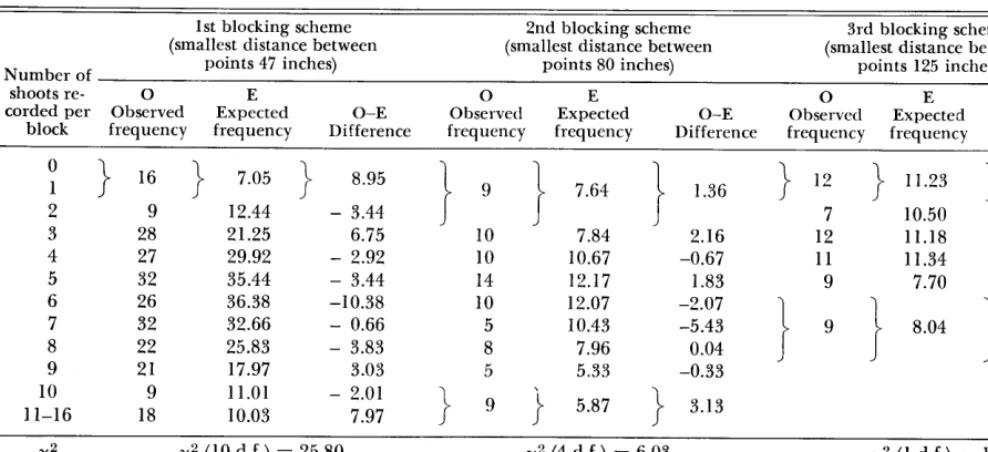
Table 1. x2 tests to determine required spacing of sampling points for the Matopos thornveld.
1st blocking scheme
(smallest distance between 2nd blocking scheme 3rd blocking scheme Number of points 47 inches)
(smallest distance between
points 80 inches) (smallest distance between points 125 inches)
shoots re- 0 E 0 E 0 E
corded per Observed Expected O-E Observed Expected O-E Observed O-E
block frequency frequency Difference frequency frequency Difference frequency frequency Expected Difference
; } 16 } 7.05 } 8.95 \ g 1 7.64 1 1.36 } l2 } llez3 } o*77
2 3 4 5 6
7 8 9 10 11-16
9
28 27 32 26 32 22 21 9 18
12.44 21.25 29.92 35.44 36.38 32.66 25.83 17.97 11.01 10.03
- 3.44 6.75 - 2.92 - 3.44 -10.38 - 0.66 - 3.83 3.03 - 2.01 7.97
J
J
J
10 7.84 2.16
10 10.67 -0.67
14 12.17 1.83
10 12.07 -2.07 5 10.43 -5.43 7.96 0.04
5 5.33 -0.33
5.87 3.13
7 12
11 9
9
10.50 -3.50 11.18 0.82 11.34 -0.34
7.70 1.30
0.96
X2 x2 (10 d.f.) = 25.80 x2 (4 d.f.) = 6.03 x2 (1 d.f.) = 1.59
P P < 0.01 P> 0.1 P > 0.2
likely to exceed the kill for very small and for very large h and the opposite will be true for inter- mediate h. Disagreement with the null hypothesis may be tested by means of a x2 test. Before x2 is calculated, it must be ascertained that all expected frequencies Gil, achieve a minimum value of 5. If one or more of the k, are smaller than 5, suc- cessive values of h must be grouped and the cor- responding ki, and kill must each be pooled, until all groups comply with this requirement. A sig- nificant x2 value is proof that, at this spacing of points, the null hypothesis is not true. Especially if the deviations of observed from expected fre- quencies follow the trend described above, there is hope that increasing the distance between stations will rectify the situation.
There is a difficulty about the correct number of degrees of freedom for x2. If after grouping there are c frequency classes, then x2 has between (c-l) and (c-5) d e g rees of freedom. A significant result with (c - 1) degrees of freedom establishes significance beyond all doubt, while nonsignifi- cance is ascertained if x2 with (c- 5) degrees of free- dom is not significant. In other cases, there is un- certainty. A test that is both more powerful and always yields a clearcut result is being developed.
The above test was applied to data collected at Matopos Research Station, Rhodesia. The site is located in the “thornveld” which has been de- scribed by Rattray (1957). At this site, the distribu- tion of plants is distinctly aggregated. Only peren- nial grasses were recorded. Nine hundred and sixty sampling points were located in 48 parallel lines, all 2 ft distant from their nearest neighbor, while the distance between points in the same line
was 80 inches. Points in alternate lines were staggered.
Three blocking schemes were used and, for each of these, a different spacing of points was simulated by considering different sets of selected points only. In the first blocking scheme all points were con- sidered, in the second all points in every third line were taken into account and in the third, every alternate point of every fourth line was used in such a way that points in alternate lines were staggered. For the first two schemes, blocks of four points were made up as compact as possible, while the blocks of the third scheme contained two points, one from each of two adjoining lines.
The results for Themeda triandra, the species with the highest relative density, are given in Table 1. The other major species gave similar results. The groupin g of neighboring frequencies in the table serves to achieve the required mini- mum expected frequency of 5.
It appears that, for this type of vegetation, sta- tions should not be as closely spaced as in the first blocking scheme.
P.C.Q. SAMPLING 375
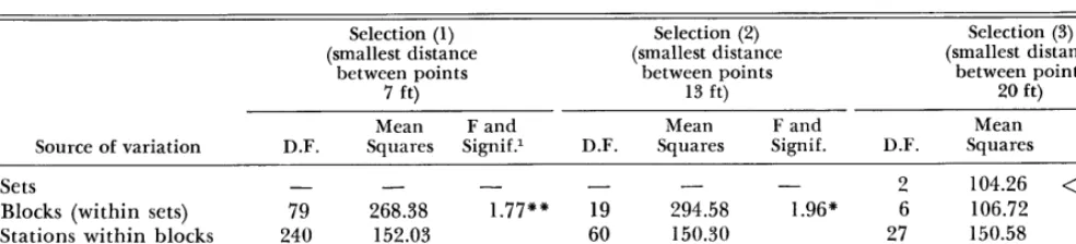
Table 2. Analysis of variance of distance measurements (the unit in the analysis is d,, in cm).
Source of variation
Sets
Blocks (within sets)
Stations within blocks Quarters within stations
Selection (1) Selection (2) Selection (3)
(smallest distance (smallest distance (smallest distance
between points between points between points
7 ft) 13 ft) 20 ft>
Mean F and Mean F and Mean F and
D.F. Squares Signif? D.F. Squares Signif. D.F. Squares Signif.
- - - - - - 2 104.26 < 1
79 268.38 1.77”” 19 294.58 1.96” 6 106.72 0.71 (NS)
240 152.03 60 150.30 27 150.58 2.26””
- - - - -
- 108 66.52
I* and ** signify significant at P < 0.05 and P < 0.01 respectively. (NS) means nonsignificant.
Chi-squared tests the disagreement between the ris and fi. The number of degrees of freedom for x2 is (u - 1). If the probability level corresponding to x2 is small then there is strong evidence that the distribution of the species is heterogeneous. The cure is then to divide the sampling area into strata which, regards the distribution of species, are uniform within themselves, to calculate fi and v(Fi) for each stratum and, possibly, to pool these quantities over all strata.
This test was applied to the Matopos data. The sampling area was divided into four patches, each 48 ft x 66 ft 8 inches in size. For Themeda triandra
and using the points of blocking scheme 3, the test yielded x2 (3 degrees of freedom) = 3.33; 0.3 < P < 0.5. Similar results were obtained for the other major species. There is thus no evidence that the species distribution on this site is not homogeneous.
While these two tests cope with what are thought to be the more common situations in which care must be exercised with the statistical evaluation of P.C.Q. data from systematic samples, many more may be listed. Examples are systematic vari- ation in clump size together with a tendency for some species to occupy specific positions in the clumps and periodicity in the distribution of spe- cies. Operators should always be on the lookout for like trends.
It is not recommended that both x2 tests are always applied for all species. Once an operator is familiar with a certain vegetation type, he will be able to judge adequately what distances to use between points and close scrutiny of the data will reveal marked heterogeneity of distributions of species without recourse to formal tests of signifi- cance. It is perhaps reassuring that, by arguments similar to those of Yates (1949), v(Fi) computed from systematic sample data, if at all biased, is likely to be an over-estimate of the variance of Fi.
Distribution of the Mean Distance with Systematic Sampling
By arguments similar to those of the previous section, the D1,. corresponding to a systematic
sampling method may be uncorrelated, in which case the estimate of variance of
D .
. is the same as for a random sample, nl.v(D..) = [ i (d,.-d..)‘]/(n-l)n.
k:l
In accordance with the discussion of intraclass correlation by Scheffe (1959), correlation between the D,. may be discovered by means of an analysis of variance. The procedure is illustrated for the Matopos data. Different distances between sam- pling points were simulated by using only selected points. The selections used were, (1) all points of every third line, (2) alternate points of every sixth line, and (3) every third point of every ninth line. The corresponding minimum distances be- tween sampling points are
7,
13, and 20 ft re- spectively. For each selection, square blocks of four adjacent points were made up and the analy- ses of variance of Table 2 were obtained.The F value in the “blocks” line of the analysis is the ratio of the mean squares for blocks and stations within blocks and tests whether the mean distances at stations in the same blocks are cor- related. If the blocks mean square is the larger of the two, this indicates positive correlation.
Also for selection 3, the four distance measure- ments at each station were included in the analysis. The F value in the “stations within blocks” line is the ratio of the last two mean squares. If the mean square for stations within blocks is the larger, as in this case, a positive correlation between the distances measured at the same station is indicated.
The results for the Matopos site are much as would generally be expected. Close spacing of points leads to a positive correlation between the mean distances at neighboring stations, which disappears as stations are further apart. At Matopos, all evidence of correlation between the D,;. dis- appears at a spacing of 20 ft (selection 3). The positive correlation between the four distances measured at the same station, which was found at Matopos, may be expected to crop up in most types of grassland. This is the reason for estimating the variance of D.. from the mean distances per sta- tion instead of the distances per quarter. Com- putationally, it is easiest to replace the d,. in the formula for v(D . .) by the total distances per station and d.. by their mean and to divide the answer by 16.
The analysis of variance procedure is strictly valid only if the D,. are normally distributed, in which case absence of correlation may be taken to indicate independence of the D,.. In very dense cover the distribution of the mean distance per station is likely to be positively skew, tending to symmetry as the vegetation gets less dense. For- tunately, the P.C.Q. method is most useful in places with sparse vegetation. Also, the analysis of vari- ance is reasonably “robust” as far as mild devia- tions from normality are concerned. In cases of doubt, a cumulative frequency diagram should be plotted on normal probability paper. The Matopos data agreed reasonably well with the assumption of normality.
Considering all the evidence together, it appears that, for the Matopos thornveld, valid estimates of the variances of the Fi and D . . may be obtained from a systematic sample, provided that sampling points are about 20 ft or more apart.
Statistical Analysis
Because of the many designs of experiments and surveys which may yield P.C.Q. data, it is not possible to present a general method of statistical analysis. The best that can be done is to mention a few of the considerations and techniques which can play a part in the construction of a suitable method for a given set of data. Attention has been confined to the univariate case, i.e. the analysis of the relative density of one species at a time.
With standard designs, involving adequate repli- cation, it is usually possible to employ analysis of variance techniques with the relative density of a
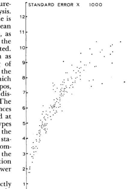
STANDARD ERROR X 1000
‘1 , , , RELATIVE DENSITY
0 .I .2 .3 .4 5
FIG. 4. Relationship between relative density and its standard error. Data from four Matopos grazing experiments.
species as variable. Similarly, analysis of covariance may be done, with as covariable for example the relative density of the species at the initiation of the experimental treatments. Two necessary con- ditions for a valid analysis of variance are that the variable is normally distributed and that its vari- ance is constant. As will be seen later, the nor- mality assumption will often be met reasonably well. Difficulties are likely to arise with the second condition.
The analysis of four grazing experiments at Matopos necessitated the computation of the v(Fi) corresponding to 192 relative densities, each based on observations at 1,000 stations. Fig. 4 shows the observed relationship between these fi and v(Fi) (actually, lOOO[v(Fi)]’ was plotted). No data were available for fi greater than 0.5. The obvious similarity with the behavior of binomial data is not surprising and may be expected to occur in general.
P.C.Q. SAMPLING 377
This is not likely to be very important in practice, unless treatment differences approach the order of obviousness. Although there may then be little interest in tests of significance, confidence intervals remain important and a suitable variance-stabiliz- ing transformation should be applied. Care must be taken that the normality assumption is not violated over-much after such a transformation. It is unfortunate that, in contrast to binomial variables, there is no known, theoretically justified transformation. Furthermore, the relationship of Fig. 4 may well vary with the type of vegetation. In some cases, distribution-free methods may be useful.
In practice, considerations of space and/or time will often severely limit the level of replication. By making use of the v(Fi), it is possible to devise methods for the construction of confidence in- tervals for the relative densities corresponding to the different treatments in an unreplicated experi- ment and to test for treatment differences. The interpretation of the results of such an analysis is complicated by the fact that treatment effects and “plot” effects are completely confounded. While every care can be exercised to minimize plot effects (choice of a uniform experimental area; careful management; selection of a suitable vari- able for analysis, such as the difference between the relative density of a species at the beginning and at the end of the experiment), there always remains a component of the variability between plots which is beyond the experimenter’s control. Before the methods which are described below can be employed, there must be some reassurance that this component is relatively small.
One commonly encountered unreplicated situ- ation arises when it is desired to investigate a time trend at a single site under constant manage- ment. Here the difficulty is not one of plot effects but of confounding between time and seasonal effects. Replication can never help to overcome this hurdle and neither does staggering of the start- ing times eliminate all difficulties. All the same, it may be interesting to study the combined effect of time and season, in which case the following methods can be applied.
From the definition of Fi,
Fi =
( i Xi,<)
/
4n,
kzland the Central Limit Theorem of probability theory, it follows that Fi is asymptotically normally distributed with increasing n. Provided that n is large and that the standard error of fi is small compared with both fi itself and the quantity (1 - fi), statistical treatment of Fi as a normally dis- tributed variable with known variance equal to v(Fi) should give a good approximation. As will
be seen later, n will often need to be very large, in order to achieve the desired degree of precision.
There is an obvious analogy between the sta- tistical methods which are applicable in an experi- mental situation where the members of a (sub)set of q treatment means are based on different num- bers of replications, rl, r2, . . . , r,, say and those that can be used when dealing with a set of nor- mally and independently distributed variables, Y1, Ye, . . . , Y,, with unknown means, ~1, ~2, . . . , pq, and known variances a12, a22, . . . , uq2. Let the error variance for the hypothetical experiment be c2, estimated with f degrees of freedom, and assume that the residuals in the underlying mathematical model are normally and independently distributed. If now the ri are such that r1al2 = r2a22 = . . . = r,a, 2 = fl2 then, as f tends to inifinity, the distribu- tions of the means in the experiment tend to the dis- tributions of the corresponding Yi. Thus confidence regions for functions of the pi can be constructed and tests of significance of such functions can be performed as for the experiment, merely replacing the ri by u2/ui2 and taking the degrees of freedom for error to be infinitely many. The unknown constant u2 plays no important role, since it is usually equally represented in the test statistic and in the variable of which the test statistic is hy- pothesized to be a realization. In practice there- fore, the ri can be replaced by wi = 1 /ai the “weights” of the Yi.
The above trick is never essential for the deriva- tion of a result. It may, however, provide a useful shortcut. Identifying the Yi with relative densities and the (+i2 with the corresponding v(Fi), the follow- ing are some results with obvious applications to P.C.Q. problems.
(I) On the assumption that pl = p2 = . . .=pq= E,L, the weighted mean,
u = [
$l(wiYi)]/(il-i)p
is the best (minimum variance) linear un- biased estimate of p and u may be seen as a realization of a normally distributed vari- able with variance equal to
l/(
s_i>~
(II) The weighted sum of squared deviations from u,
(III)
(IV)
(V
so that the null hypothesis p1 = p2 = . . . = ,..ts may be tested against the class of all alternative hypotheses by means of a x2 test. The above sum of squares may be partitioned
orthogonally into several (up to (q - 1)) com- ponents, to test selected hypotheses, anal- ogous to the partitioning of the treatment sum of squares of an experiment with un- equal replication (e.g. fitting polynomials of increasing degree).
A contrast y among the means is defined as a linear function of the pi,
Y = Si (aipi) , i=l
with known constant coefficients subject to the condition
iai=O. I=1
An unbiased estimate of y is provided by
’ =
$+
(aiyi) , I=1and c is a realization of a normally dis- tributed variable C with variance equal to
U2(C) = i (ai2Vi2) . I=1
The quantity C2/a2(c) has non central x2 dis- tribution with one degree of freedom and non centrality parameter equal to y2/02(c), so that the null hypothesis y = 0 may be tested against the alternative y # 0 by means of a x2 test.
If the contrasts of interest are such that the corresponding tests of (IV) don’t fit into the scheme described in (III), some workers may prefer to use the S method of Scheffk (1959). Adapted to the P.C.Q. problem, the pro- cedure is to declare a contrast significantly different from zero or not at the level (Y, according as the interval (c - sa(c), c + SU(C)) excludes, respectively includes the value zero. The constant s is calculated from s2 = x”a;(q - l), where x%;(q - 1) is the upper (Y point of the central x2 distribution with (q - 1) degrees of freedom. If the only con- trasts of interest are pairwise differences be- tween the expectations, a more powerful testing procedure may be obtainable by adapting one of the existing procedures for testing the differences between the means in an experiment with unequal replication. An example of such a method is the multi- ple range test of Duncan (1957).
Mutatis mutandis, the analysis of distance mea-
surements is similar to that of relative densities. Provided that n is large, equating v(D . .) to the true population variance should give good approxi- mations.
If the variables in an analysis correspond to suc- cessive samples, collected in the same sampling area, care must be exercised that these samples are independent. If random sampling is used, a fresh randomization is required for each sample. With systematic placement of points, two successive sets of observations at the same site will not be strictly independent, unless the distance between points is increased a lot. The points at the second sampling can then be fitted between those of the first, at a sufficient distance for the two samples to be inde- pendent.
Random Line Sampling
If the sampling area is too small to accommodate the required number of points at a sufficiently large distance apart and if the randomization of points over the sampling area is too laborious, then random line sampling can be used. Sampling posi- tions are chosen at random along a number of parallel lines, like the compass lines of the system- atic sample, and a new randomization is used at each sampling time. Stratification by lines or sec- tions of lines is easily achieved. The selected sam- pling positions are located on the ground by means of a tape-measure.
Interpretation of Results
Grassland vegetation may change in any com- bination of the following two ways:
(I) the relative preponderance of all species, in terms of numbers of shoots and plants per unit area, remains constant but the overall cover alters and
(II) the overall cover, in terms of total number of shoots and plants per unit area over all species, remains constant but the relative preponderance of one or more species changes.
A significant increase or decrease in d.. with time may reasonably be taken to mean that (I) has taken place, while a significant change in one or more of the fi would indicate the occurrence of (II). On this basis, four grazing experiments at Matopos were analyzed, using the statistical tech- niques described above. The results will, in due course, be published elsewhere but it is perhaps relevant to quote the officer in charge of these experiments who wrote:
P.C.Q. SAMPLING
379
RELATIVE DENSITY
0 .I .2 .3 $4 .5
FIG. 5. Relationship between relative density and n,, the num- ber of points for 10% precision.
Number of Stations Required
From each pair of values (fi, v(Fi)), obtained from a sample size n, it is an easy matter to obtain an estimate of np, the average number of sampling positions required to estimate E(Fi) with such a degree of precision that the 95% fiducial limits are given by fi * pfi/ 10. It may be readily verified that this estimate is provided by
The nl have been computed for each of the 192 sets of values of n, fi, and v(Fi) which were obtained from the Matopos grazing experiments. Fig. 5 gives the relationship between nl and relative density.
Insufficient is known about possible relation- ships between relative density and its standard error to be able to postulate a law defining the corresponding relationship between nl and rela- tive density. It is quite possible that this will vary a little with locality. Despite these objections, an
lC c PERCENT PRECISION (=I0 PI
IC
RELATIVE DENSITY
0 .I .2 .3 .4 .5
FIG. 6. Relationship between relative density and percentage precision for a fixed number of strikes (t).
attempt was made to fit a curve to the points of Fig. 5. The only restrictions imposed are that it must be asymptotic to the nl axis, it must pass through the point nl = 0, relative density = 1, it must be continuous and without points of in- flection. Of all the many types of curves tried, the best fit was achieved by
For different relative densities, the nr, values may be estimated from this equation by dividing the corresponding nl by p2. An estimate of p with n’ stations is provided by (nl/n’)*.
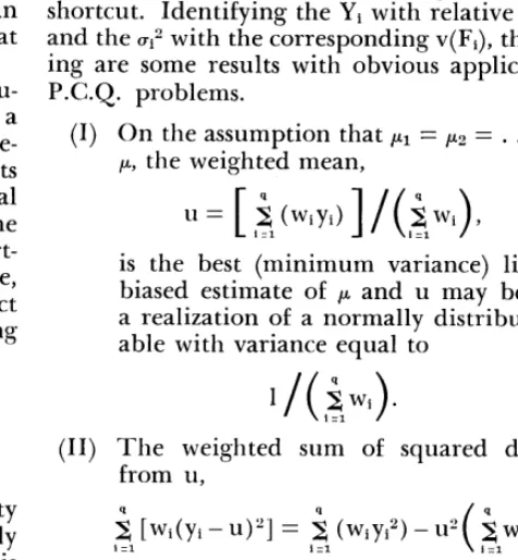
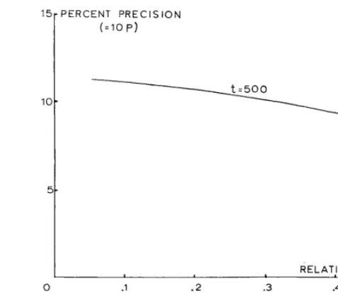
Another way to present these results is in terms of the precision achieved if sampling is continued until a species of interest has been recorded a given number of times. If this total number of “strikes” is denoted by t and provided t is not too small, then for any corresponding fi, p may be estimated from
p = 2(nlfi/t)“,
where nl is obtained from Fig. 5.
Dix (1961) claims that quite good precision is achieved for t = 30. For the Matopos data, Fig. 6 gives the relationship between fi and p for t = 500. For other values of t the corresponding p values may be found by multiplying the values of Fig. 6 by (500/t)*. Th us the precision for t = 30 is obtained by multiplication by 4.08.
easily constructed for that specific type and may manuscript and of Mr. W. B. Cleghorn, Mr. T. C. D. be readily updated from time to time. Kennan, and Mr. R. P. Denny with the collection of data
In order to achieve the desired degree of pre- in the field, is gratefully acknowledged. cision if E(Fi) is small, many points are needed.
If much interest exists in rare species, then multi- LITERATURE CITED
phase sampling, as described by Yates (1949), is ‘OTTAM’ G”. AND J* T’ ?R?’ 1956. The use of distance recommended. In each phase, all but a number of measures In phytosoclologlcal sampling. Ecology 37:451- selected grass species are ignored. By this strategem, 460.
the relative density of a rare species is artificially COTTAM, G., J. T. CURTIS, AND B. W. HALE. 1953. Some ‘increased within its sampling phase. sampling persed individuals. characteristics Ecology 34: 74 of a population l-757. of randomly dis-
The required number of sampling positions to Drx, R. L. 1961. An application of the point-centred estimate mean distances with sufficient precision quarter method to the sampling of grassland vegetation. will usuallv be smaller than the number needed J. Range Manage. 14:63-69.
for precise hstimates of relative densities. DUNCAN, D. B. 1957. Multiple range tests for correlated and heteroscedastic means. Biometrics 13: 164-176.
Acknowledgments RATTRAY, J. M. 1957. The grasses and grass associations
Thanks are due to the Director, Dep. of Research and of Southern Rhodesia. Rhodesia Agric. J. 54:197-233. Specialist Services, Ministry of Agriculture, Rhodesia, for SCHEFFI?, H. 1959. The analysis of variance. Ch. 7. Wiley permission to publish this article. The assistance of Mrs. & Sons, London.
G. Gough, Mrs. L. Murray, Mr. N. H. Judge, and Mr. D. YATES, F. 1949. Sampling methods for censuses and sur- White with the data processing and preparation of the veys. Ch. 3, 7. Charles Griffin & Co., London.
An Aerial Method of Dispensing
Ground Squirrel Bait
REX E. MARSH1
Associate Specialist, Department of Animal Physiology, University of California, Davis
Highlight
A need for improving and updating rodent-control methodology prompted this study of the use of aircraft for baiting destructive populations of ground squirrels. Both spot and strip baiting by air were effective when ap plied in narrow swaths at a rate of 6 lb/swath acre. The aerial technique of dispersing bait gave good control when the ground squirrel population was foraging extensively for seed. The bait need be applied to only a fraction of the ground surface of squirrel-infested rangeland.
Metodo Aereo de Dispersar Cebo Envenenado para Ardillas (Citellus beecheyi)
Resumen2
El uso de aeroplanos para diseminar cebos de granos envenenados para controlar las ardillas (Citellus beecheyi), l I gratefully acknowledge assistance given by Richard Dana,
California Department of Agriculture; Bert Collins and Herb Hagen, Department of Fish and Game; and many others of those agencies. Also deeply appreciated is the excellent cooperation and assistance of the Agricultural Commissioners and their staffs in Kern, Merced, and Tulare Counties. For their part in making this study possible, I am particularly indebted to Agricultural Com- missioner Earl Kalar and Vertebrate Pest Biologist Verne McGlothlen, San Luis Obispo County; and Richard May- born, aircraft pilot for most of the applications.
2Por Ing. Edmund0 L. Aguirre, Dep. de Zootecnia, ITESM, Monterrey, N.L., Mexico.
una de las plagas mayores de 10s pastizales en varios estados de1 Oeste de Estados Unidos, ha probado ser efectivo en California.
Los cebos a&-eos toman ventaja de la habilidad forrajera de las ardillas para localizar y consumir una cantidad fatal de cebos ampliamente dispersados al voleo. Semillas de avena tratadas con 0.070 a 0.113% de fluoracetato de sodio (1080) a 6 lb p or una franja de un acre dio buen control de ardillas si se aplica al tiempo cuando las ardillas estuvieran alimenthndose con semillas y no estuvieran invernando. El cebo necesita ser aplicado a tinicamente una fracci6n de la superficie de1 suelo si se hate al tiempo de1 aAo cuando toda la poblaci6n de ardillas esti activa en la superficie ali- mentandose extensivamente con semillas; entonces ambos cebos en franjas y manchones al voleo por avi6n dan re- sultados satisfactorios, usando las franjas mas estrechas conseguidas por el avi6n.
Otras especies de roedores son afectados por el tratamiento en grados variables, pero no hubo evidencia de perdidas de aves de caza. Los invertebrados y el clima son factores importantes que contribuyen a la degradacibn de1 cebo. La tecnica no es un remedio universal para el control de las ardillas, mas bien es un metodo avanzado que sera titil en muchas situaciones. Si es usado con discreci6n la dis- tribuci6n de cebos por avi6n es una herramienta segura y de valor para el control de ardillas en 10s potreros de1 Oeste.
This study was made principally to determine the effectiveness of aerial baiting for controlling ground squirrels (Citellus spp.), a major pest of