Jacobian Coordinates on Genus 2 Curves
Huseyin Hisil1
and Craig Costello2 1
Yasar University, Izmir, Turkey
Microsoft Research, Redmond, USA
Abstract. This paper presents a new projective coordinate system and new explicit algorithms which together boost the speed of arithmetic in the divisor class group of genus 2 curves. The proposed formulas generalise the use of Jacobian coordinates on elliptic curves, and their application improves the speed of performing cryptographic scalar multiplications in Jacobians of genus 2 curves over prime fields by an approximate factor of 1.25x. For example, on a single core of an Intel Core i7-3770M (Ivy Bridge), we show that replacing the previous best formulas with our new set improves the cost of generic scalar multiplications from 243,000 to 195,000 cycles, and drops the cost of specialised GLV-style scalar multiplications from 166,000 to 129,000 cycles.
Keywords: Genus 2, hyperelliptic curves, explicit formulas, Jacobian coordinates, scalar multiplication.
1
Introduction
Motivated by the popularity of low-genus curves in cryptography [33, 26, 27], we put forward a new system of projective coordinates that facilitates efficient group law computations in the Jacobians of hyperelliptic curves of genus 2. This paper combines several techniques to arrive at explicit formulas that are significantly faster than those in previous works [29, 12]. The two main ingredients we use in the derivation
are:-– The generalisation of Jacobian coordinates from the elliptic curve setting to the hyperelliptic curve setting: these coordinates essentially cast affine points into projective space according to theweights ofxandyin the defining curve equation. While applying Jacobian coordinates to elliptic curves is straightforward, their application to hyperelliptic curves requires transferring the x-y weightings into weightings for the Mumford coordinates. As it does for the x-y
coordinates in genus 1, this projection naturally balances the Mumford coordinates to facilitate substantial simplifications in the projective genus 2 group law formulas.
– The adaptation of Meloni’s “co-Z” idea [32] to the genus 2 setting. Although originally proposed in the context of addition-only (e.g. Fibonacci-style) chains, this approach can also be used to gain performance in the more meaningful context of binary addition chains. Moreover, this idea is especially advantageous when used in conjunction with Jacobian coordinates.
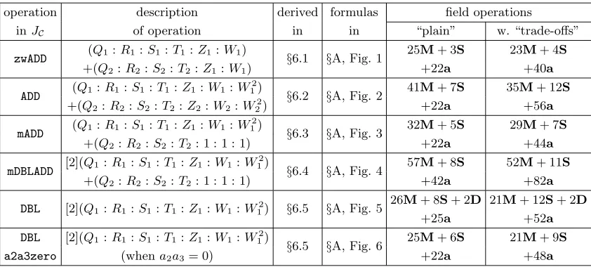
into an existing genus 2 scalar multiplication routine that uses the formulas from [29] or [12]. (We give a better indication of the improvements over previous formulas by reporting concrete implementation numbers in Section 8.) As well as the reduction in field multiplications indicated in Table 1, the explicit formulas in this paper also require far fewer field additions than those in [29] and [12]. We note that the biggest relative difference occurs in themDBLADDcolumn: among other things, this difference results from the combination of the new coordinate system with the extension of Meloni’s idea [32], which allows us to computemDBLADDoperations independently of the curve constants. On the other hand, when such curve constants are zero, certain operations in this paper become even faster (relatively speaking): for example, on the two special families exhibiting endomorphisms used in [8], the doubling formulas in [29] and [12] save 2D, while the new operation count reported forDBLin Table 1 saves 3S+ 2Dto drop down to 21M+ 9S.
authors DBL mADD mDBLADD
Lange [29] 32M+ 7S+ 2D 36M+ 5S 68M+ 12S+ 2D
Costello-Lauter [12] 30M+ 9S+ 2D 36M+ 5S 66M+ 14S+ 2D
This work 21M+ 12S+ 2D 29M+ 7S 52M+ 11S
Table 1.Field operation counts obtained in this work, versus two previous works, for the most common operations incurred during cryptographic scalar multiplications in Jacobians of genus 2 curves of the form C/K: y2
= f(x), where f(x) is of degree 5 and the characteristic of K is greater than 5.
While the formulas in this paper target Jacobians of imaginary genus 2 curves, Gaudry showed in [20] that one can perform cryptographic scalar multiplications much more efficiently in the special case that the Jacobian of the curve C/K hasK-rational two-torsion, by instead working on an associated Kummer surface. To illustrate the difference between working on the Kummer surface and working in the full Jacobian group, Gaudry’s analogous operation counts are a blazingly fast 6M+ 8S for DBL and 16M+ 9S for mDBLADD. Referring back to Table 1, it is clear that raw scalar multiplications on the Kummer surface will remain unrivalled by those in the full Jacobian group. However, there are several cryptographic caveats related to the Kummer surface that justify the continued exploration of fast algorithms for traditional arithmetic in the Jacobian. Namely, Kummer surfaces do not support genericadditions, so while they are extremely fast in the realm of key exchange (where such additions are not necessary), it is not yet known how to efficiently use the Kummer surface in a wider realm of cryptographic settings, e.g. for general digital signatures3
. Furthermore, the absence of generic additions complicates the application of endomorphisms [8, §8.5], and from a more pragmatic standpoint, also prevents the use of standard precomputation techniques that exploit fixed system parameters (those of which give huge speedups in practice, even over the Kummer surface [8,§7.4]). Thus, all genus 2 implementations that either target signature schemes, use endomorphisms, or optimise the use of precomputation, are currently required to work in the full Jacobian group4
; and in all of these cases, the formulas in this paper will now offer the most efficient route. The upshot is that in popular practical scenarios the most efficient genus 2 cryptography is likely to result from a hybrid combination of operations on the Kummer surface and in the full Jacobian group. We illustrate this in Section 8 by benchmarking genus 2 curves in the context of ephemeral elliptic curve Diffie-Hellman (ECDHE) with perfect forward secrecy: to exploit the best of both worlds, Alice’s multiplications of the public
3
At least one exception here, as Gaudry points out, is the hashed version of ElGamal signatures [20, §5.3]
4
generator P by each one of her ephemeral scalars a can make use of our new explicit formulas (and offline precomputations onP) in the full Jacobian, and her resulting ephemeral public keys [a]P can then be mapped onto the corresponding Kummer surface, whose speed can be exploited by Bob in the computation of the shared secret [b]([a]P).
A set of Magma [9] scripts verifying all of the explicit formulas and operation counts in this paper are publicly available at
http://research.microsoft.com/en-us/downloads/37730278-3e37-47eb-91d1-cf889373677a/ ; and a complete mixed-assembly-and-C implementation of all explicit formulas and scalar multi-plication routines is publicly available at
http://hhisil.yasar.edu.tr/files/hisil20140527jacobian.tar.gz .
2
Preliminaries
For ease of exposition, we immediately restrict to the most cryptographically common case of genus 2 curves, whereCis an imaginary hyperelliptic curve over a fieldKof characteristic greater than 5. (In terms of a general coverage of all genus 2 curves, we mention the interesting leftover scenarios in Section 9.) Every such curve can then be written as
C/K:y2
=f(x) :=x5 +a3x
3 +a2x
2
+a1x+a0, (1)
where we note the absence of anx4
term inf(x); it can always be removed via a trivial substitution thanks to char(K)6= 5.
LetJC denote the Jacobian of C. We assume that we are working with a general point P ∈
JC(K), whose Mumford representation
5
P ↔(u(x), v(x)) = x2
+qx+r, sx+t
∈K[x]×K[x]
↔(q, r, s, t)∈A4(K) (2) encodes two affine points (x1, y1),(x2, y2)∈ C(K), where we assume thatx16=x2so that these two points are not the same, nor are they the hyperelliptic involution of one another. The Mumford coordinates (q, r, s, t) ofP are uniquely determined according to u(x1) =u(x2) = 0, v(x1) =y1 andv(x2) =y2. That is,
q=−(x1+x2), r=x1x2, s=
y1−y2
x1−x2
, t= x1y2−y1x2
x1−x2
. (3)
From (1), (2) and (3), it is readily seen that
v(x)2
−f(x) = 0 in K[x]/hu(x)i, (4) from which it follows that such general points P lie in the intersection of two hypersurfaces over
K [12,§3], given as
S0 : r s 2
+q3
−(2r−a3)q−a2
=t2 −a0, S1 : q s
2 +q3
−(3r−a3)q−a2
= 2st−r(r−a3)−a1.
(5)
These hypersurfaces can be used to simplify expressions that arise in our derivation, and are especially useful in our derivation of unified formulas (see §A.3). We note that a more simple relation is found by takingrS1−qS0.
5
We adopted the notation (q, r, s, t) over (u1, u0, v1, v0) to avoid additional subscripts/superscripts when
working with distinct elements in JC. This eases the synchronisation between, and readability of, the
Our driving motivation for improving the explicit formulas for arithmetic in the Jacobian is the application of enhancing the fundamental operation in curve-based cryptosystems: the scalar multiplication [k]P of an integer k ∈ Z by a general point P in JC. Such scalar multiplications
are computed using a sequence of point doubling and addition operations, and so a common way of comparing different sets of addition formulas is to tally the number of field multiplications (denoted byM), field squarings (denoted byS), and field additions (denoted bya) that each point operation incurs. In cryptographic contexts, the input and output points are typically required to be in their unique affine form, whilst intermediate computations are carried out in projective space to avoid inversions. Thus, the most commonly reported operation counts include:DBL, which refers to the addition of a Jacobian point in projective form to itself; ADD, which refers to the addition between two distinct points in projective form;mADD, which refers to themixed addition between a projective point and an affine point; and mDBLADD, which refers to the combined doubling of a projective point and subsequent addition of the result with an affine point.
As is done in [29,§5-6], in this paper we focus on deriving formulas for the most common cases of arithmetic inJC. This set of formulas is enough to perform and benchmark scalar multiplications
in JC, since the possible input/output cases are extremely dense amongst all possible scenarios,
i.e. for random input points P and scalars k, the cases not covered by these formulas have an exponentially small probability of being encountered in the scalar multiplication routine (see [29, §1.2] for a similar discussion). Nevertheless, the set of formulas we present are still far from a completeand cryptographically adequate coverage, so it is important to distinguish exactly which input/output cases they do apply to. We clarify this in Assumption 1 below, and return to this discussion in§7.3.
Assumption 1 (General points and operations in JC.) Throughout this paper, we assume
that all input and output points are “general” points in JC: we say that P ∈ JC is general if the
Mumford representation of P encodes two distinct affine points (x1, y1)and(x2, y2) on C, where
x1 6=x2. Moreover, all operations in this paper are of the form P1+P2 =P3, where we assume that P1,P2 andP3 are general points and that we are in one of two cases: (i) either P1=P2, in which case we are computing the “doubling” P3 = [2]P1, where we further assume that neither of the two x-coordinates encoded byP1 coincide with the two encoded by P3, or (ii) that of the six points encoded byP1,P2 andP3, no two share the samex-coordinate.
3
Extending Jacobian coordinates to Jacobians
Let λ be a nonzero element in K. Over fields of large characteristic, Jacobian coordinates have proven to be a natural and efficient way to work projectively on elliptic curves in short Weierstrass form E/K: y2
= x3
+ax+b. Indeed, in cryptographic contexts, using the triple (λ2
X :λ3
Y :λZ)∈ P(2,3,1)(K) to represent the affine point (X/Z2
, Y /Z3 )∈ A2
(K) on E was suggested by Miller in his seminal 1985 paper [33, p. 424], and his comment that this representation “appears best” still holds true after decades of further exploration: Jacobian coordinates (and extended variants) remain the most efficient way to work on such general Weierstrass curves [5]. Moreover, the weightings wt(x) = 2 and wt(y) = 3 are the orders of the poles of the functionsx
andy at the point at infinity onE.
In the context of imaginary hyperelliptic curves of the form C/K :y2
=x5 +a3x
3 +a2x
2
+a1x+a0, the analogous weightings are
wt(x) = 2, and wt(y) = 5, (6)
under which the affine point (X/Z2
, Y /Z5 )∈A2
(K) is represented by the triple (λ2
X :λ5
Y :λZ)∈ P(2,5,1)(K), which lies on
C/K :Y2 =X5
+a3X 3
Z4 +a2X
2
Z6
+a1XZ 8
+a0Z 10
Indeed, the weights wt(x) = 2 and wt(y) = 5 are the orders of the poles ofxandy at the (unique) point at infinity onC. Since we perform arithmetic using the Mumford coordinates inJC, rather
than thex-ycoordinates onC, we transfer the above weightings across to the Mumford coordinates via Equation (3), which yields
wt(q) = wt(x), wt(r) = 2·wt(x), wt(s) = wt(y)−wt(x), wt(t) = wt(y). (8) Combining (6) and (8) then gives
wt(q) = 2, wt(r) = 4, wt(s) = 3, wt(t) = 5, (9) which suggests the use of (λ2
Q:λ4
R:λ3
S: λ5
T :λZ)∈P(2,4,3,5,1)(K) to represent the affine point
(q, r, s, t) =
Q Z2,
R Z4,
S Z3,
T Z5
∈A4(K). (10)
Equation (10) is at the heart of this paper. We found these weightings to be highly advantageous for group law computations: the Mumford coordinates balance naturally under this projection, and significant simplifications occur regularly in the derivation of the corresponding explicit formulas. This coordinate system is referred to as Jacobian coordinates in this paper. We note that, in line with Assumption 1, we will not work with the full projective closure of the affine part in P(2,4,3,5,1)(K), but rather with the affine patch whereZ 6= 0.
Just as in [29, §6], we found it useful to introduce an additional coordinate (independent of
Z) in the denominator of the two coordinates corresponding to thev-polynomial in the Mumford representation. So, in addition to the Jacobian coordinate Z, we include the coordinateW and use the projective six-tuple (λ2
Q:λ4
R: λ3
µS:λ5
µT :λZ:µW) to represent the affine point
(q, r, s, t) =
Q Z2,
R Z4,
S Z3W,
T Z5W
∈A4(K) (11)
for some nonzeroµinK. This coordinate system is referred to as auxiliary Jacobian coordinates in this paper.
Remark 1. We note the distinction between the above coordinate weightings and the weightings used by Lange, which were also said to “generalise the concept of Jacobian coordinates . . . from elliptic to hyperelliptic curves” [29,§6]. In terms of the first projective coordinateZ, Lange used (q, r, s, t) = Q/Z2
, R/Z2
, S/Z3
, T /Z3
. Although these weight theu- andv-polynomials of a point with the same (Jacobian) weightings as thex- andy-coordinates on an elliptic curve, the derivation of the weightings in (10) draws a closer analogy with the use of Jacobian coordinates in genus 1. This is why we dubbed the weightings used in this work as “Jacobian coordinates”.
4
Adopting the “co-Z” approach
With the aim of improving addition formulas on elliptic curves, Meloni [32] put forward a nice idea that is particularly suited to working in Jacobian coordinates. In the explicit addition of two elliptic curve points (X1:Y1: Z1) and (X2: Y2:Z2) inP(2,3,1)(K), which respectively correspond to the points (X1/Z
2 1, Y1/Z
3
1) and (X2/Z 2 2, Y2/Z
3 2) inA
2
(K), Meloni observed that almost all expressions of the formZi
1Z
j
2 can completely vanish ifZ1=Z2. That is, the sum of the points (X1:Y1:Z1) and (X2: Y2: Z1) can be written as an expression of the form (X3Z
6 1 : Y3Z
9 1 : Z3Z
3
1), which is projectively equivalent to (X3:Y3: Z3); hereX3 andY3 depend only onX1, Y1, X2 and Y2, so now it is onlyZ3 that depends onZ1. Since two projective points are unlikely to share the same
this update would incur a significant overhead. The observation that is key to making this “co-Z” approach advantageous is that, in the context of scalar multiplications, these updated values (or the main subexpressions within them) are often already computed in the previous operation [32, p. 192], so this update can be performed either for free, or with a much smaller overhead.
Meloni did not apply his idea to classical “double-and-add” style addition chains, but sub-sequent papers [30, 23] showed how his approach could be used to enhance performance in such binary chains. (These chains are preferred in cryptographic contexts due to the ease of using them to achieve various side-channel resistant properties inside a scalar multiplication routine.) In genus 2 however, successful transferral of the “co-Z” idea has not yet been achieved: the work in [28] also uses non-binary addition chains, and crucially, it was performed without access to the hyperelliptic analogue of Jacobian coordinates (those which work in stronger synergy with Meloni’s idea).
Equipped with the Jacobian coordinates described in the previous section, our adaptation of the “co-Z” approach requires that both theZ andW coordinates are the same, for two different input points. The first projective formulas we derive in Section 6 are for the “co-ZW” addition between the two pointsP1= (Q1:R1:S1:T1:Z1:W1) andP2= (Q2:R2:S2:T2:Z1:W1), and this routine is then used as a subroutine for all subsequent operations (except for standalone doublings).
5
Arithmetic in affine coordinates with new common subexpressions
The explicit formulas for arithmetic in genus 2 Jacobians are significantly more complicated than their elliptic curve counterparts, so it is especially useful to start the derivation by looking for common subexpressions and advantageous orderings in the affine versions of the formulas (i.e., before the introduction of more coordinates complicates the situation further). Our derivation follows that of [12], but it is important to point out that the resulting affine formulas have been refined by grouping new subexpressions throughout; these groupings were strategically chosen to exploit the symmetries of theqand rcoordinates, and especially for the application of Jacobian coordinates that follows in Section 6.
In what follows, we give the affine formulas for general point additions and general point doublings respectively. From Section 2, recall the abbreviated notation (q, r, s, t)∈A4
(K) for the point in JC with Mumford representation (x2+qx+r, sx+t).
LetP1= (q1, r1, s1, t1),P2= (q2, r2, s2, t2) andP1+P2=:P3= (q3, r3, s3, t3) be points inJC
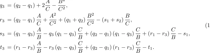
satisfying Assumption 1. The choice of the three subexpressions
A := (t1−t2) (q2(q1−q2)−(r1−r2))−r2(q1−q2) (s1−s2),
B := (r1−r2) (q2(q1−q2)−(r1−r2))−r2(q1−q2) 2
, C := (q1−q2) (t1−t2)−(r1−r2) (s1−s2)
is key to our refined derivation. The pointP3is then given by
q3 = (q1−q2) + 2
A C−
B2
C2,
r3 = (q1−q2)
A C +
A2
C2 + (q1+q2)
B2
C2 −(s1+s2)
B C,
s3 = (r1−r3)
C
B −q3(q1−q3) C
B + (q1−q3) A B −s1,
t3 = (r1−r3)
A
B −r3(q1−q3) C B −t1.
(12)
LetP1= (q1, r1, s1, t1) and [2]P1=:P3= (q3, r3, s3, t3) be points inJC satisfying Assumption 1.
Again, it is particularly useful to make use of three subexpressions:
A := q2
1−4r1+a3
q1−a2+s 2 1
(q1s1−t1) + 3q 2
1−2r1+a3
r1s1,
B := 2 (q1s1−t1)t1−2r1s 2 1,
C := q2
1−4r1+a3
q1−a2+s 2 1
s1+ 3q 2
1−2r1+a3
t1.
The pointP3 is then given by
q3 = 2
A C −
B2
C2,
r3 =
A2
C2 + 2q1
B2
C2 −2s1
B C,
s3 = (r1−r3)
C
B −q3(q1−q3) C
B + (q1−q3) A B −s1,
t3 = (r1−r3)
A
B −r3(q1−q3) C B −t1.
(13)
These formulas are used to derive projective doubling formulas in§6.5. The formulas in (12) and (13) are shown to agree with those of Costello-Lauter in§A.4 – Fig. 12.
6
Projective arithmetic in extended Jacobian coordinates
In this section we derive all of the explicit formulas that are needed for the scalar multiplication routines we describe in Section 7. The formulas are summarised in Table 2 below, where we immediately note the extension of auxiliary Jacobian coordinates discussed in Section 3 to include
W2
; it is advantageous to carry this additional coordinate between consecutive operations because it is often computed en routeto the output points already, and therefore comes for free as input into the following operation. We refer to this extended version of auxiliary Jacobian coordinates asextended Jacobian coordinates. Table 2 reports two sets of operation counts: the “plain” count, which corresponds to our deriving sets of formulas with the aim of minimising the total number of all field operations, and the “trade-offs” count, which corresponds to our deriving formulas with the aim of reducing field multiplications (M) at the expense of additional field squarings (S) and/or additions (a). Explicit algorithms and justification of the operation counts are provided (as Magma functions) in Appendix A.
If W2
is dropped from the coordinate system, and we work only with auxiliary Jacobian coordinates, (Q:R: S:T:Z :W), then we note that bothDBLandDBLa2a3zerowould require one extra squaring (in both the “plain” and “trade-off” formulas). The only other change resulting from this abbreviated coordinate system would be in the “trade-off” version of ADD, where a squaring would revert back to a multiplication. All other operation counts would remain unchanged.
Following on from the discussion in Section 4, in §6.1 we start the derivations by using the affine addition formulas in (12) to develop projective formulas forzwADD; these are then used in the derivation of the formulas for ADDin §6.2, formADDin§6.3, and formDBLADD in§6.4. Finally, we use the affine doubling formulas in (13) to develop projective formulas forDBLin §6.5.
In what follows, the square brackets that are used for the expressions [C2 ], [C4
], [C3
B], [C5
B], [C], [B], and [B2
operation description derived formulas field operations
inJC of operation in in “plain” w. “trade-offs”
zwADD (Q1:R1:S1:T1:Z1:W1) §6.1 §A, Fig. 1 25M+ 3S 23M+ 4S
+(Q2:R2:S2:T2 :Z1:W1) +22a +40a
ADD (Q1:R1:S1:T1:Z1:W1:W 2 1)
§6.2 §A, Fig. 2 41M+ 7S 35M+ 12S
+(Q2:R2:S2:T2:Z2:W2:W 2
2) +22a +56a
mADD (Q1:R1:S1:T1:Z1:W1:W 2 1)
§6.3 §A, Fig. 3 32M+ 5S 29M+ 7S
+(Q2:R2:S2:T2: 1 : 1 : 1) +22a +44a
mDBLADD [2](Q1:R1:S1:T1:Z1:W1:W 2 1)
§6.4 §A, Fig. 4 57M+ 8S 52M+ 11S
+(Q2:R2:S2:T2: 1 : 1 : 1) +42a +82a
DBL [2](Q1:R1:S1:T1:Z1:W1:W 2
1) §6.5 §A, Fig. 5
26M+ 8S+ 2D 21M+ 12S+ 2D
+25a +52a
DBL [2](Q1:R1:S1:T1:Z1:W1:W 2 1)
§6.5 §A, Fig. 6 25M+ 6S 21M+ 9S
a2a3zero (whena2a3= 0) +22a +48a
Table 2.A summary of the explicit formulas derived in this section for various operations in the Jacobian,
JC, of an imaginary hyperelliptic curveC/Kof genus 2, with char(K)>5.
6.1 Projective co-ZW addition (zwADD)
Let P1 = (Q1: R1: S1: T1: Z1: W1), P2 = (Q2: R2: S2: T2: Z1: W1), and P1 +P2 =:
P3= (Q3:R3:S3:T3:Z3: W3: W32) represent three points in JC satisfying Assumption 1. We
emphasize thatP1andP2need not containW 2
1, which is why both are given in auxiliary Jacobian coordinates. However, the outputP3is in extended Jacobian coordinates. The projective form of (12) in extended Jacobian coordinates corresponds to the following. We define the subexpressions
A := (T1−T2) (Q2(Q1−Q2)−(R1−R2))−R2(Q1−Q2) (S1−S2),
B := (R1−R2) (Q2(Q1−Q2)−(R1−R2))−R2(Q1−Q2) 2
, C := (Q1−Q2) (T1−T2)−(R1−R2) (S1−S2).
The pointP3 is then given by
W3 =W1[B],
Q3 = Q1C 2
−Q2C 2
+ 2AC−W2 3,
R3 = Q1
C2
−Q2
C2 +AC AC+ Q1 C2
+Q2
C2
W2 3 −S1
C3
B
−S2
C3
B
, S3 = R1
C4
−R3
+ (AC−Q3) Q1
C2
−Q3
−S1
C3
B
, T3 = R1C
4
−R3AC−R3 Q1C 2
−Q3−T1C 5
B
, Z3 =Z1[C].
(14)
This operation, referred to aszwADD, not only computesP3, but also produces the subexpressions
Q1
C2
, R1
C4
, S1
C3
B
, T1
C5
B
, Z1[C], W1[B], W12
B2
; if desired, these can be used to updateP1to be of the form
P1= (Q1:R1:S1:T1:Z1:W1:W 2 1) = (Q1C
2
:R1C 4
:S1C 3
B
: T1C 5
B
:Z1[C] :W1[B] :W 2 1
B2
),
so that it now has the same Z, W, and W2
coordinates as P3. The combination of the zwADD operation and this update will be denoted using the syntax
where P′
1 is the updated (but projectively equivalent) version of P1. Explicit formulas for this operation are provided in Appendix A – Figure 1; they can be computed in 25M+ 3S+ 22a, or at the expense of more field additions, in 23M+ 4S+ 40ausing trade-offs.
6.2 Projective addition (ADD)
Rather than producing lengthy formulas for additions, we use a simple construction that exploits zwADD. Let P1 = (Q1: R1: S1: T1: Z1: W1: W
2
1), P2 = (Q2: R2: S2: T2: Z2: W2: W 2 2), and P1+P2 =: P3 = (Q3: R3: S3:T3:Z3: W3:W32) represent three points in JC satisfying
Assumption 1. We can then cross-multiply to define the points in auxiliary Jacobian coordinates
P′
1:= Q1
Z2 2
:R1
Z4 2
:S1
Z3 2W2
:T1
Z5 2W2
:Z1[Z2] : W1[W2]
, P′
2:= Q2
Z2 1
:R2
Z4 1
:S2
Z3 1W1
:T2
Z5 1W1
:Z2[Z1] : W2[W1]
.
Observe thatP′
1=P1andP2′ =P2, but thatP
′
1andP
′
2now share the sameZandW coordinates. This means that we can use the zwADD operation defined in §6.1 to computeP3 = P1+P2 as (P3, P1′′) := P
′
1+P
′
2. Observe that P′′
1 = P1, and that P
′′
1 will share the same Z, W, and W 2 coordinates as P3. We note that this update of P1 into P1′′ can be useful in the generation of lookup tables [30], but is generally not useful during the main loop. Explicit formulas for this operation are provided in Appendix A – Figure 2; they can be computed in 41M+ 7S+ 22a, or at the expense of more field additions, in 35M+ 12S+ 56ausing trade-offs.
6.3 Projective mixed addition (mADD)
In a similar way, let P1 = (Q1:R1: S1:T1:Z1: W1:W12), P2 = (Q2:R2: S2:T2: 1 : 1 : 1), and P1+P2 =: P3 = (Q3: R3: S3:T3:Z3: W3:W32) represent three points in JC satisfying
Assumption 1. This time we only need to update P2 into P2, which is performed in auxiliary′ Jacobian coordinates as
P′
2:= Q2
Z2 1
:R2
Z4 1
:S2
Z3 1W1
: T2
Z5 1W1
: [Z1] : [W1]
,
where we observe thatP1 andP2′ now have the sameZ and W coordinates. Subsequently, using thezwADDoperation from§6.1 allowsP3=P1+P2to be computed by (P3, P1) :=′ P1+P2. Explicit′ formulas are provided in Appendix A – Figure 3; they can be computed in 32M+ 5S+ 22a, or at the expense of more field additions, in 29M+ 7S+ 44ausing trade-offs.
6.4 Projective mixed doubling-and-addition (mDBLADD) LetP1= (Q1: R1:S1:T1:Z1:W1:W
2
1),P2= (Q2:R2:S2:T2: 1 : 1 : 1), and [2]P1+P2=:
P3= (Q3:R3:S3:T3:Z3:W3:W 2
3), represent three points inJC satisfying Assumption 1. To
compute [2]P1+P2, we schedule the higher level operations in the form (P1+P2)+P1(see [15] and [30] for the same high level scheduling). This means thatmDBLADDcan be computed using anmADD operation before azwADDoperation. (Subsequently, we must also assume thatP1, the intermediate pointP1+P2, and the output point [2]P1+P2=:P3= (Q3:R3:S3:T3:Z3:W3: W
2
3) represent three points in JC satisfying Assumption 1.) Following §6.2 and §6.3, this can be computed in
57M+ 8S+ 42a, or at the expense of more additions, in 52M+ 11S+ 82ausing trade-offs. Explicit formulas for themDBLADDoperation are provided in Appendix A – Figure 4.
6.5 Projective doubling (DBL)
Jacobian coordinates corresponds to the following. We define the subexpressions
A := Q1 Q 2 1−4R1
+ Q1−(a2/a3)Z 2 1
a3Z 4 1
W2 1 +S
2 1
(Q1S1−T1) + 3Q2
1−2R1+a3Z 4 1
W2 1R1S1,
B := 2 (Q1S1−T1)T1−2R1S 2 1,
C := Q1 Q 2
1−4R1+ Q1−(a2/a3)Z 2 1
a3Z 4 1
W2 1 +S
2 1
S1+ 3Q2
1−2R1+a3Z 4 1
W2 1T1.
We can then writeP3 as
W3 =W1[B],
Q3 = 2AC−W 2 3,
R3 = (AC) 2
+ 2Q1
C2
W2 3 −2S1
C3
B
,
S3 = R1
C4
−R3
+ (AC−Q3) Q1
C2
−Q3
−S1
C3
B
, T3 = R1C
4
−R3AC−R3 Q1C 2
−Q3−T1C 5
B
, Z3 =Z1[C].
(15)
TheDBLoperation not only computesP3, but also produces the subexpressionsQ1
C2
,R1
C4 , S1 C3 B
,T1
C5
B
, Z1[C], W1[B],W12
B2
; if desired, these can be used to updateP1 into
P1= (Q1:R1:S1: T1:Z1:W1: W 2 1) = Q1
C2
:R1
C4
:S1
C3
B
:T1
C5
B
:Z1[C] :W1[B] : W2 1
B2
,
in order to share the same Z, W, and W2
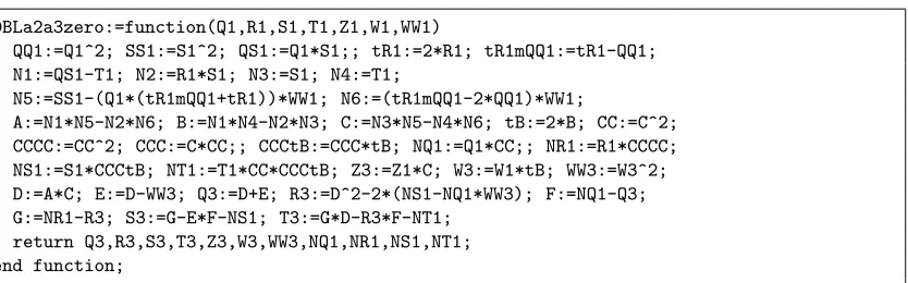
coordinates with P3. Explicit formulas for the DBL operation are provided in Appendix A – Fig. 5; they can be computed in 26M+ 8S+ 2D+ 25a, or at the expense of more additions, in 21M+ 12S+ 2D+ 52a using trade-offs. We define the operationDBLa2a3zeroto be a doubling in the special case that the curve constantsa2anda3are zero. Explicit formulas in this case are provided in Appendix A – Fig. 6; they can be computed in 25M+ 6S+ 22a, or at the expense of more additions, in 21M+ 9S+ 48ausing trade-offs.
7
Implementation
We chose two different curves to showcase the explicit formulas derived in the previous section, both of which target the 128-bit security level.
The first curve was found in the colossal point counting effort undertaken by Gaudry and Schost [22]. From a security standpoint, it is both twist-secure and it is not considered to be special (e.g. it has a large discriminant); from a performance standpoint, it was chosen over the arithmetically advantageous fieldFp withp= 2127−1, and with optimal cofactors such that the
curve supports a Gaudry-style Kummer surface implementation [20]. This is the same Kummer surface that was used to set speed records in [8] and [3]. We chose the Jacobian of this curve to illustrate the performance that is gained when using our new formulas inside a general “double-and-add” scalar multiplication routine.
The second curve supports a 4-dimensional GLV decomposition [19]. Over prime fields, requiring 4-dimensional GLV imposes that the Jacobian has CM by a special field – in this case it is Q(ζ5). This (specialness) means that we cannot hope to find a twist-secure curve over a particular prime, but rather that we must search over many primes. In the same vein as [8, §8.3], we also wanted this curve to support a rational Gaudry-style Kummer surface. This curve is defined over the prime fieldp= 2128
CM byQ(ζ5) overFp is twist-secure with optimal cofactors6. This curve was chosen to exhibit the
performance that is gained when using our new formulas inside a GLV-style multiexponentation; in particular, each step of the multiexponentation requires only anmDBLADDoperation, and this is where our explicit formulas offer the largest relative speedup over the previous ones.
7.1 Working on the Gaudry-Schost Jacobian
Letp= 2127
−1, and define the following constants inFp: a:= 11, b:=−22, c:=−19,d:=−3,
e := 1 +p−833/363 and f := 1−p−833/363. For the Rosenhain invariants λ= ac bd, µ =
ce df,
ν= ae
bf, the curve
CRos/Fp : y
2
=x(x−1)(x−λ)(x−µ)(x−ν) is such that #JCRos = 2
4
·r and #JC′
Ros = 2
4
·r′, wherer and r′ are 250- and 251-bit primes
respectively [22], and where C′
Ros is the quadratic twist of CRos. The coefficient of x4 in CRos is
α=−(1 +λ+µ+ν), and we choose to zero it under the transformationϕ : CRos→C˜,(x, y)7→
(x−α/5, y). The resulting curve, ˜C, has a coefficient of x3
which is a fourth power in Fp; let
it be u−4
, where we chose u = 19859741192276546142105456991319328298. We can then use the map ψ : ˜C → C,(x, y) 7→ (x·u2
, y·u5
) to work with the isomorphic curve C/Fp : y2 =
x5 +x3
+a2x2+a1x+a0, where the coefficient ofx3 being 1 saves a multiplication inside every point doubling7
. We use the name Jac1271for the Jacobian JC, and use the name Kum1271 for
the associated Kummer surfaceK– this is defined by the above constantsa, b, c, d(see [20]). In Section 8 we report two new sets of implementation numbers on Jac1271. Firstly, we benchmark a generic scalar multiplication, using both the old and the new formulas, to illustrate the performance boost given by this work in the general case. In addition, we benchmark a fixed-basescalar multiplication, which uses the new formulas and takes advantage of precomputations on a public generator to give large speedups onJac1271. In the context of ECDHE, this second benchmark corresponds to the “key gen” phase, which compliments the performance numbers for the “shared secret” scalar multiplications onKum1271in [8] and [3]. (We discuss some caveats related to this Jacobian/Kummer combination in §7.3.) To tie these two sets of performance numbers together, we also benchmark the numbers for computing the map from Jac1271 onto Kum1271, which was made explicit in the AVIsogenies library [7], and for general points in JCRos
is given as
Ψ : JCRos→ K, (x
2
+qx+r, sx+t)7→(X:Y:Z:T),
where
X =a r(µ−r)(λ+q+ν)−t2
, Y =b r(νλ−r)(1 +q+µ)−t2
, Z=c r(ν−r)(λ+q+µ)−t2
, T =d r(µλ−r)(1 +q+ν)−t2
. (16) For practical scenarios like ECDHE, it is fortunate that we only need the map in this direction, as the pullback map fromKtoJCRos is much more complicated [20,§4.3]. Since we compute inJC
(rather thanJCRos), we actually need to compute the composition ofΨ with (ψϕ)
−1
, which when extended to general points inJC is
(ψϕ)−1
: JC →JCRos , (x
2
+qx+r, sx+t)7→(x2
+q′x+r′, s′x+t′),
with
q′ =u−2
q+ 2α/5, r′ =u−4
r+α/5q′−(α/5)2
, s′=u−3
s, t′=u−5
t+α/5s′.
6
It is relatively straightforward to show that ifJC has CM byQ(ζ5) and full rational two-torsion, then
eitherJC orJC′ must contain a point of order 5; thus, the optimal cofactors are 16 and 80. 7
If the coefficient ofx3
Assuming that the input point inJC is in extended Jacobian coordinates, the operation count for
the full mapΨ′=Ψ(ψϕ)−1
fromJC toKis 1I+ 31M+ 2S+ 19a(see Figure 10 in Appendix A.2);
we benchmark it alongside the scalar multiplications in Section 8.
To draw a fair comparison against prior works, we inserted our formulas into the software made publicly available by Boset al. [8], which itself employed the previous best formulas. (We tweaked both sets of formulas for Jac1271 to take advantage of the constant a3 = 1.) This software computes the scalar multiplications onJac1271using a left-to-right signed sliding window recoding [1] with a window size of w = 5, where the lookup table consists of 8 points and is constructed exactly as in [30,§4]. The timings are presented in Section 8.
7.2 Working on the Jacobian of a GLV curve
Letp= 2128
−7689975 and define C/Fp : y2 =x5+ 710. The Jacobian groupsJC andJC′ have cardinalities #JC = 24·5·rand #JC′= 24·r′, where
r= 2252
+ 375576928331233691782146792677798267213584131651764404159
/5 and
r′
= 2252
−375576928331887882475846226038533397089218679777223482485
are both prime.
The implementation of a 4-dimensional GLV scalar multiplication inJC follows that which is
described in [8, §6]; again, we wrapped their GLV software around both their old and our new formulas for a fair comparison – we note that both instances were made to use the above curve, which we refer to asGLV128c.
Practically speaking, it does not make as much sense to benchmark GLV128c in the same ECDHE style as we discussed for Jac1271 and Kum1271. If there is enough storage to exploit a long-term public generator P, then the presence of endomorphisms is essentially redundant in the key gen phase, since multiples of P can then be precomputed offline without using an endomorphism. On the shared secret side, where variable-base scalar multiplications are performed on fresh inputs, our implementations show that a 4-dimensional decomposition on GLV128c is still slightly slower than a Kummer surface scalar multiplication, so in the case of ECDHE, it is likely to be faster on both sides to stick with the combination of Jac1271 and Kum1271. Nevertheless, there could be scenarios where it makes sense to use the endomorphism on GLV128c(e.g. for a signature verification), and still make use of the maps between the full Jacobian group and the associated Kummer surface. In this case, the map in (16) and the pullback map in [20,§4.3] can be exploited analogously to the case ofJac1271, keeping in mind that the maps would pass through the Jacobian of the Rosenhain form ofC.
Timings for a 4-dimensional GLV variable-base scalar multiplication onGLV128c using both the old and the new explicit formulas are given in Section 8.
We note that in all scalar multiplication routines, i.e. in both fixed- and variable-base scalar multiplications on Jac1271 and in 4-dimensional multiexponentiations on GLV128c, we always found it advantageous to convert the lookup table elements from extended Jacobian coordinates to affine coordinates using Montgomery’s simultaneous inversion method [34]. This “decision” is generally made easier in genus 2, where the difference between mixed additions and full additions is greater, and the relative cost of a field inversion (compared to the rest of the scalar multiplication routine) is much less than it is in the elliptic curve case. Finally, we note that the single conversion of the output point from Jacobian to affine coordinates comes at a cost of 1I+ 10M+ 1S(see Figure 9 in Appendix A.2).
7.3 A disclaimer: the difficulties facing constant-time, exception-free scalar multiplications in JC
Jacobians is closely related to Assumption 1. We note that these are not the same implementation-level difficulties pointed out in [3, §1.2]; indeed, while the Kummer surface implementations reported in [3] and [8] run in constant time, a truly constant-time genus 2 implementation that does not use the Kummer surface is yet to be documented in the literature.
More specifically, there are scalar recoding algorithms (cf. [24, 16]) that seemingly make it possible to implement theJac1271orGLV128croutines such that scalar multiplications on random inputs will run in constant time with probability exponentially close to 1. However, in order to guard against active adversaries and to be consideredtrulyconstant-time, the routines should be guaranteed to execute identically and run correctly for all combinations of integer scalars and input points; this means the explicit formulas must be able to handle input combinations inJC
that are not “general” in the sense of Assumption 1. Although explicit formulas can be developed for each of these special cases, their culmination into an efficient and truly constant-time scalar multiplication algorithm remains an important open problem.
8
Results
In this section we present the timings of the routines described in the previous section. All of the benchmarks were performed on an Intel Core i7-3770M (Ivy Bridge) processor at 3.4 GHz with hyperthreading turned off and over-clocking (“turbo-boost”) disabled, and all-but-one of the cores switched off in BIOS. The implementations were compiled with gcc 4.6.3 with the-O2flag set and tested on a 64-bit Linux environment. Cycles were obtained using the SUPERCOP [6] toolkit and then rounded to the nearest 1,000 cycles.
The primary purpose of our benchmarks is to compare the performance of scalar multiplications in genus 2 Jacobians using both the old and new sets of explicit formulas. Table 3 reports that a generic scalar multiplication on Jac1271 using the explicit formulas in this paper gives a factor 1.25x improvement over one that uses the previous best formulas; this is the approximate speedup that one can expect when adopting extended Jacobian coordinates on any imaginary hyperelliptic curve of genus 2 over a large prime field. Table 4 reports that a 4-dimensional GLV multiexponentiation routine using the explicit formulas in this paper gives a factor 1.29x improvement over the same routine that calls the previous explicit formulas. We note that the benchmarked implementations of the new formulas always used the “plain” versions (see Table 2), since these proved to be more efficient than the “trade-off” versions in our implementations.
curve coordinates formulas from cycles
Jac1271 homogeneous [12, 8] 243,000
Jac1271 ext. Jacobian this work 195,000
Table 3.Benchmarking the old and new explicit formulas in the context of a generic scalar multipli-cation onJac1271.
curve coordinates formulas from cycles
GLV128c homogeneous [12, 8] 166,000
GLV128c ext. Jacobian this work 129,000
Table 4.Benchmarking the old and new explicit formulas in the context of a 4-GLV scalar multipli-cation onGLV128c.
side-channel attacks. We also benchmarked a fixed-base scalar multiplication with a much smaller 1KB lookup table, but it ran in 87,000, which when combined with theΨ′ map, is not faster than
the scalar multiplication onKum1271from [3].
ECDHE operation details curve coordinates implementation cycles
key gen fixed-base scalar mul Jac1271 ext. Jacobian this work 36,000
Ψ′
map - - this work (and [7]) 4,000
shared secret variable-base scalar mul Kum1271 theta [20] Bernsteinet al.[3] 91,000
Table 5.The performance of genus 2 in ECDHE on the Gaudry-Schost curve [22].
We reiterate that, to get the performance numbers in Tables 3 and 4, and those forkey genin Table 5, we modified the software made publicly available by Boset al.[8] to be able to call both sets of explicit formulas. This software already included routines for general scalar multiplications, 4-GLV scalar multiplications, and the fixed-base scenario. To complete the benchmarks in Table 5, we ran the publicly available software from [3] on our hardware.
9
Related scenarios
We conclude by mentioning some related cases of interest, for which the analogue of (extended) Jacobian coordinates and/or the co-Z idea could also be applied. The takeaway message of this section is that, while we focussed on the most common instance of genus 2 curves, the ideas in this work have the potential to boost the speed of arithmetic in other scenarios too.
– Real hyperelliptic curves. In Section 2 we immediately specialised to theimaginary case, where C/K is hyperelliptic of degree 5 with one point at infinity. The complimentary case in genus 2, where the curve is of degree 6 and has two points at infinity [17], has received less attention in papers pursuing high performance, since it is slightly slower than the imaginary case [14]. Moreover, it is often the case (at least among the scenarios of practical interest) that a degree 6 model contains a rational Weierstrass point and can therefore be transformed to a degree 5 model (e.g. the family in [21,§4.4]). On the other hand, there are some scenarios where this transformation is not always possible, so it is of interest to see how efficient projective arithmetic can be made in the real case, and whether analogues of the ideas in this work can be carried across successfully.
– Pairings. Genus 2 pairings are also likely to benefit from Jacobian coordinates. Roughly speaking, the explicit formulas in this paper inherently compute the additional components (i.e. the Miller functions) that are required in a pairing computation. However, the resulting savings would not be as drastic, as the operations in JC are dominated by extension field operations
– Low characteristic / higher genus. The specialisation of Jacobian coordinates to low characteristic genus 2 curves and the extension to higher genus imaginary hyperelliptic curves follows analogously. However, the motivation in both directions is nowadays stunted by their respective security concerns. Nevertheless, it could be worthwhile to see how much faster the arithmetic in these cases can become when using Jacobian coordinates.
– The RM families.We benchmarked the new explicit formulas in two scenarios; on a non-special “generic” curve, and on a curve with very non-special CM that subsequently comes equipped with an endomorphism. A third option comes from the families with explicit RM in [21], which perhaps achieves the best of both worlds in genus 2: they are constructed to have an endomorphism, but are much more general than the CM curve we used. This generality dispels any security concerns associated with special curves, and moreover allows them to be found over a fixed prime field. Thus, at the 128-bit security level, one could find such a curve over
p= 2127
−1 that facilitates both 2-dimensional GLV decomposition on its Jacobian and which supports a (twist-secure) Kummer surface. It would then be very interesting to benchmark the new explicit formulas on one of these families, where the GLV routine would again make a higher relative frequency of calls to the fastmDBLADDroutine.
Acknowledgements. We thank Joppe Bos, Michael Naehrig, Benjamin Smith, and Osmanbey Uzunkol for their useful comments on an early draft of this work.
References
1. R. M. Avanzi. A note on the signed sliding window integer recoding and a left-to-right analogue. In H. Handschuh and M. A. Hasan, editors,Selected Areas in Cryptography, volume 3357 ofLecture Notes in Computer Science, pages 130–143. Springer, 2004.
2. R. Barbulescu, P. Gaudry, A. Joux, and E. Thom´e. A heuristic quasi-polynomial algorithm for discrete logarithm in finite fields of small characteristic. In P. Q. Nguyen and E. Oswald, editors, EUROCRYPT, volume 8441 ofLecture Notes in Computer Science, pages 1–16. Springer, 2014. 3. D. J. Bernstein, C. Chuengsatiansup, T. Lange, and P. Schwabe. Kummer strikes back: new DH speed
records. IACR Cryptology ePrint Archive, 2014:134, 2014.
4. D. J. Bernstein and T. Lange. Faster addition and doubling on elliptic curves. InASIACRYPT 2007, volume 4833 ofLNCS, pages 29–50. Springer, 2007.
5. D. J. Bernstein and T. Lange. Explicit-formulas database, accessed 2 Jan, 2014. http://www.hyperelliptic.org/EFD/.
6. D. J. Bernstein and T. Lange. eBACS: ECRYPT Benchmarking of Cryptographic Systems, accessed 28 September, 2013. http://bench.cr.yp.to.
7. G. Bisson, R. Cosset, and D. Robert. AVIsogenies – a library for computing isogenies between abelian varieties, November 2012. URL: http://avisogenies.gforge.inria.fr.
8. J. W. Bos, C. Costello, H. Hisil, and K. Lauter. Fast cryptography in genus 2. In T. Johansson and P. Q. Nguyen, editors,EUROCRYPT, volume 7881 ofLecture Notes in Computer Science, pages 194–210. Springer, 2013, full version available at: http://eprint.iacr.org/2012/670.
9. W. Bosma, J. Cannon, and C. Playoust. The Magma algebra system. I. The user language.J. Symbolic Comput., 24(3-4):235–265, 1997. Computational algebra and number theory (London, 1993). 10. E. Brier and M. Joye. Weierstraß elliptic curves and side-channel attacks. InPublic Key Cryptography,
pages 335–345. Springer, 2002.
11. D. V. Chudnovsky and G. V. Chudnovsky. Sequences of numbers generated by addition in formal groups and new primality and factorization tests. Advances in Applied Mathematics, 7(4):385–434, 1986.
12. C. Costello and K. Lauter. Group law computations on Jacobians of hyperelliptic curves. In A. Miri and S. Vaudenay, editors,Selected Areas in Cryptography, volume 7118 ofLecture Notes in Computer Science, pages 92–117. Springer, 2011.
13. O. Diao and M. Joye. Unified addition formulæ for hyperelliptic curve cryptosystems. In3rd Workshop on Mathematical Cryptology (WMC 2012) and 3rd International Conference on Symbolic Computation and Cryptography (SCC 2012), pages 45–50, 2012.
15. X. Fan and G. Gong. Efficient explicit formulae for genus 2 hyperelliptic curves over prime fields and their implementations. In C. Adams, A. Miri, and M. Wiener, editors,Selected Areas in Cryptography, volume 4876 ofLecture Notes in Computer Science, pages 155–172. Springer Berlin Heidelberg, 2007. 16. A. Faz-Hern´andez, P. Longa, and A. H. Sanchez. Efficient and secure algorithms for GLV-based scalar multiplication and their implementation on GLV-GLS curves. In J. Benaloh, editor,CT-RSA, volume 8366 ofLecture Notes in Computer Science, pages 1–27. Springer, 2014.
17. S. D. Galbraith, M. Harrison, and D. J. Mireles Morales. Efficient hyperelliptic arithmetic using balanced representation for divisors. In A. J. van der Poorten and A. Stein, editors, ANTS, volume 5011 ofLecture Notes in Computer Science, pages 342–356. Springer, 2008.
18. S. D. Galbraith, J. Pujol`as, C. Ritzenthaler, and B. A. Smith. Distortion maps for supersingular genus two curves. J. Mathematical Cryptology, 3(1):1–18, 2009.
19. R. P. Gallant, R. J. Lambert, and S. A. Vanstone. Faster point multiplication on elliptic curves with efficient endomorphisms. In J. Kilian, editor,CRYPTO, volume 2139 ofLecture Notes in Computer Science, pages 190–200. Springer, 2001.
20. P. Gaudry. Fast genus 2 arithmetic based on Theta functions. Journal of Mathematical Cryptology JMC, 1(3):243–265, 2007.
21. P. Gaudry, D. R. Kohel, and B. A. Smith. Counting points on genus 2 curves with real multiplication. In D. H. Lee and X. Wang, editors,ASIACRYPT, volume 7073 ofLecture Notes in Computer Science, pages 504–519. Springer, 2011.
22. P. Gaudry and E. Schost. Genus 2 point counting over prime fields.J. Symb. Comput., 47(4):368–400, 2012.
23. R. R. Goundar, M. Joye, A. Miyaji, M. Rivain, and A. Venelli. Scalar multiplication on Weierstraß elliptic curves from Co-Zarithmetic. J. Cryptographic Engineering, 1(2):161–176, 2011.
24. M. Hamburg. Fast and compact elliptic-curve cryptography. Cryptology ePrint Archive, Report 2012/309, 2012. http://eprint.iacr.org/.
25. H. Hisil. Elliptic curves, group law, and efficient computation. PhD thesis, Queensland University of Technology, 2010.
26. N. Koblitz. Elliptic curve cryptosystems. Mathematics of computation, 48(177):203–209, 1987. 27. N. Koblitz. Hyperelliptic cryptosystems. Journal of cryptology, 1(3):139–150, 1989.
28. V. Kovtun and S. Kavun. Co-Z divisor addition formulae in jacobian of genus 2 hyperelliptic curves over prime fields. Cryptology ePrint Archive, Report 2010/498, 2010. http://eprint.iacr.org/. 29. T. Lange. Formulae for arithmetic on genus 2 hyperelliptic curves. Appl. Algebra Eng. Commun.
Comput., 15(5):295–328, 2005.
30. P. Longa and A. Miri. New composite operations and precomputation scheme for elliptic curve cryptosystems over prime fields. In R. Cramer, editor,Public Key Cryptography PKC 2008, volume 4939 ofLecture Notes in Computer Science, pages 229–247. Springer Berlin Heidelberg, 2008. 31. D. Lubicz and D. Robert. A generalisation of Miller’s algorithm and applications to pairing
computa-tions on abelian varieties. Cryptology ePrint Archive, Report 2013/192, 2013. http://eprint.iacr.org/. 32. N. Meloni. New point addition formulae for ECC applications. In C. Carlet and B. Sunar, editors,
WAIFI, volume 4547 ofLecture Notes in Computer Science, pages 189–201. Springer, 2007.
33. V. S. Miller. Use of elliptic curves in cryptography. In H. C. Williams, editor,CRYPTO, volume 218 ofLecture Notes in Computer Science, pages 417–426. Springer, 1985.
A
Appendix
Section A.1 of this appendix provides justifications for all claimed operation counts with explicit algorithms. Section A.2 provides explicit algorithms for the coordinate conversions and maps used in this work. Section A.3 proposes new unified addition formulas/algorithms and their corresponding operation counts. Finally, Section A.4 provides Magma [9] scripts to show how the proposed formulas compare to the existing formulas in the literature.
A.1 Main algorithms and operation counts
It is convenient to state few operation counting conventions before providing the explicit algo-rithms.
1. It is assumed thata2/a3 is precomputed and cached whenevera36= 0. A multiplication bya3 anda2/a3are counted as 1Deach. (See also§7.1 for rescalinga3to 1 or to a “small” constant.) 2. The operationszwADD,mADD,mDBLADD,ADD, andDBLare all capable of producing the expression
W2
3, which can be fed the nextDBLroutine asW 2
1 to save an extra 1Sfor each of the doublings. To simplify the concept, the operations are counted simply on the extended coordinates (Q:R:S: T:Z: W:W2
).
3. A further extension of the new coordinates by Z2 , Z4
, Z3
W, Z5
W, with an analogy to Weierstrass form elliptic curves (see [11]), speeds up the generic additions. One technicality is that only Z2
andZ4
are used by the doubling algorithm. Therefore, an extension byZ2 and
Z4
is more attractive in the context of scalar multiplication. The concept of re-additions can also help in optimizing the scalar multiplication (see [4]). However, as mentioned in§7.2, it is even better to normalize the look-up table both byW andZcoordinates and to make calls to either DBLormDBLADDin each iteration of the main loop. Therefore, the new coordinates are never extended by any of the extra coordinatesZ2
,Z4 ,Z3
W, orZ5
W in our implementation. The explicit algorithms for the operationszwADD,ADD,mADD,mDBLADD, andDBLare provided as Magma [9] functions, respectively, in order to justify a first step of the claimed operation counts as follows. The coordinate namesQ1,R1,S1, T1,Z1, W1,W2
1,Q2,R2, S2,T2,Z2,W2, W 2 2, Q3,
R3,S3,T3,Z3,W3,W2
3 are denoted byQ1,R1,S1,T1,Z1,W1,WW1,Q2,R2,S2,T2,Z2,W2,WW2,Q3, R3,S3, T3, Z3,W3, WW3, respectively. The constants (a2/a3) and a3 are denoted by (a2/a3)and a3, respectively. The script in Figure 6 is a revised version of DBLwhich assumes thata2a3= 0.
zwADD:=function(Q1,R1,S1,T1,Z1,W1,Q2,R2,S2,T2)
N3:=Q1-Q2; N4:=R1-R2; N6:=S1-S2; N5:=T1-T2; N1:=N3*Q2-N4; N2:=N3*R2; A:=N1*N5-N2*N6; B:=N1*N4-N2*N3; C:=N3*N5-N4*N6; CC:=C^2; CCCC:=CC^2;
CCC:=C*CC;; CCCB:=CCC*B; NQ1:=Q1*CC; NQ2:=Q2*CC; NR1:=R1*CCCC; NS1:=S1*CCCB; NS2:=S2*CCCB; NT1:=T1*CC*CCCB; Z3:=Z1*C; W3:=W1*B; WW3:=W3^2; D:=A*C; E:=NQ2-NQ1-D; F:=E+WW3; Q3:=D-F; R3:=WW3*(NQ1+NQ2)-D*E-NS1-NS2; G:=NQ1-Q3; H:=NR1-R3; S3:=H+F*G-NS1; T3:=H*D-R3*G-NT1;
return Q3,R3,S3,T3,Z3,W3,WW3,NQ1,NR1,NS1,NT1; end function;
Fig. 1.Explicit formulas forzwADD.
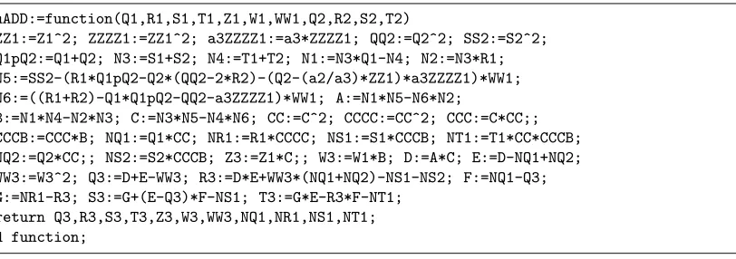
ADD:=function(Q1,R1,S1,T1,Z1,W1,WW1,Q2,R2,S2,T2,Z2,W2,WW2)
ZZ1:=Z1^2; ZZZZ1:=ZZ1^2; ZZZ1:=ZZ1*Z1;; ZZZW1:=ZZZ1*W1; NW1:=W1*W2;;; ZZ2:=Z2^2; ZZZZ2:=ZZ2^2; ZZZ2:=ZZ2*Z2;; ZZZW2:=ZZZ2*W2; NZ1:=Z1*Z2;; NQ1:=Q1*ZZ2; NR1:=R1*ZZZZ2; NS1:=S1*ZZZW2; NT1:=T1*ZZ2*ZZZW2; NQ2:=Q2*ZZ1; NR2:=R2*ZZZZ1; NS2:=S2*ZZZW1; NT2:=T2*ZZ1*ZZZW1; return zwADD(NQ1,NR1,NS1,NT1,NZ1,NW1,NQ2,NR2,NS2,NT2); end function;
Fig. 2.Explicit formulas forADD.
mADD:=function(Q1,R1,S1,T1,Z1,W1,WW1,Q2,R2,S2,T2)
ZZ1:=Z1^2; ZZZZ1:=ZZ1^2; ZZZ1:=Z1*ZZ1;; ZZZW1:=ZZZ1*W1; NQ2:=Q2*ZZ1; NR2:=R2*ZZZZ1; NS2:=S2*ZZZW1; NT2:=T2*ZZ1*ZZZW1; return zwADD(Q1,R1,S1,T1,Z1,W1,NQ2,NR2,NS2,NT2);
end function;
Fig. 3. Explicit formulas formADD.
mDBLADD:=function(Q1,R1,S1,T1,Z1,W1,WW1,Q2,R2,S2,T2)
Q3,R3,S3,T3,Z3,W3,WW3,NQ1,NR1,NS1,NT1:=mADD(Q1,R1,S1,T1,Z1,W1,WW1,Q2,R2,S2,T2); return zwADD(Q3,R3,S3,T3,Z3,W3,NQ1,NR1,NS1,NT1);
end function;
Fig. 4.Explicit formulas formDBLADD.
DBL:=function(Q1,R1,S1,T1,Z1,W1,WW1)
ZZ1:=Z1^2; ZZZZ1:=ZZ1^2; a3ZZZZ1:=a3*ZZZZ1; QQ1:=Q1^2; SS1:=S1^2; QS1:=Q1*S1;; tR1:=2*R1; tR1mQQ1:=tR1-QQ1; N1:=QS1-T1; N2:=R1*S1; N3:=S1; N4:=T1; N5:=SS1-(Q1*(tR1mQQ1+tR1)-(Q1-(a2/a3)*ZZ1)*a3ZZZZ1)*WW1;
N6:=(tR1mQQ1-2*QQ1-a3ZZZZ1)*WW1; A:=N1*N5-N2*N6; B:=N1*N4-N2*N3;
C:=N3*N5-N4*N6; tB:=2*B; CC:=C^2; CCCC:=CC^2; CCC:=C*CC;; CCCtB:=CCC*tB; NQ1:=Q1*CC;; NR1:=R1*CCCC; NS1:=S1*CCCtB; NT1:=T1*CC*CCCtB; Z3:=Z1*C;; W3:=W1*tB; WW3:=W3^2; D:=A*C; E:=D-WW3; Q3:=D+E; R3:=D^2-2*(NS1-NQ1*WW3); F:=NQ1-Q3; G:=NR1-R3; S3:=G-E*F-NS1; T3:=G*D-R3*F-NT1;
return Q3,R3,S3,T3,Z3,W3,WW3,NQ1,NR1,NS1,NT1; end function;
Fig. 5.Explicit formulas forDBL.
The claimed “trade-off” operation counts in Table 1 of Section 1 and in Table 2 of Section 6 can be precisely justified by applying the following trade-offs:
1. zwADD, zwuADD, and DBL algorithms perform a matrix resultant computation (see [12] for details) in exactly the same way
A:=N1*N5-N2*N6; B:=N1*N4-N2*N3; C:=N3*N5-N4*N6;
for which the operation count is 6M+ 3a. These operations can be traded with 5M+ 17a using the derivation based on [25, Section 3.6, Type-M4], see also [12]:
DBLa2a3zero:=function(Q1,R1,S1,T1,Z1,W1,WW1)
QQ1:=Q1^2; SS1:=S1^2; QS1:=Q1*S1;; tR1:=2*R1; tR1mQQ1:=tR1-QQ1; N1:=QS1-T1; N2:=R1*S1; N3:=S1; N4:=T1;
N5:=SS1-(Q1*(tR1mQQ1+tR1))*WW1; N6:=(tR1mQQ1-2*QQ1)*WW1;
A:=N1*N5-N2*N6; B:=N1*N4-N2*N3; C:=N3*N5-N4*N6; tB:=2*B; CC:=C^2; CCCC:=CC^2; CCC:=C*CC;; CCCtB:=CCC*tB; NQ1:=Q1*CC;; NR1:=R1*CCCC; NS1:=S1*CCCtB; NT1:=T1*CC*CCCtB; Z3:=Z1*C; W3:=W1*tB; WW3:=W3^2; D:=A*C; E:=D-WW3; Q3:=D+E; R3:=D^2-2*(NS1-NQ1*WW3); F:=NQ1-Q3; G:=NR1-R3; S3:=G-E*F-NS1; T3:=G*D-R3*F-NT1;
return Q3,R3,S3,T3,Z3,W3,WW3,NQ1,NR1,NS1,NT1; end function;
Fig. 6.Explicit formulas forDBLa2a3zero.
where the three division-by-2 operations can simply be omitted sinceA,B, and Cturn out to be orthogonal.
2. The standard M-Strade-off trick XY = ((X+Y)2 −X2
−Y2
)/2 trades 1M with 1S+ 4a wheneverX2
andY2
are computed in advance. TheM-Strade-off options have already been marked by double semicolon “;;” in the proposed algorithms.
3. Further M-Strade-off options exist through an extension of the new projective coordinates byW2
, which have been marked by triple semicolon “;;;” in the proposed algorithms. 4. FurtherM-Strade-off options exist through a selective extension of projective coordinates by
Q2 ,S2
,T2
. These trade-offs are not reflected for simplicity.
The usefulness of these trade-offs depend on the implementation. These trade-offs are not exploited in the implementation in Section 8 because the cost of additions/subtractions are not negligible in comparison with the cost of a multiplication/squaring for modular reductions using the primes of the form 2127
−1 or 2128
−c. On the other hand, these trade-offs might still be useful in other settings. Similar trade-offs were exploited in [12], so we included them in our analysis for a fair comparison.
A.2 Various explicit maps
This section provides the explicit map that converts a point from auxiliary Jacobian coordinates to affine coordinates (see Figure 9) – it uses the explicit maps in Figure 7 and Figure 8 to pass through homogeneous coordinates. In Figure 10, we provide the explicit map from Jac1271 to Kum1271discussed in§7.1.
JacToPrj:=function(Q1,R1,S1,T1,Z1,W1) n01:=W1*Z1; n02:=Z1^2; n03:=n01*n02; return Q1*n03,R1*n01,S1*n02,T1,n02*n03; end function;
Fig. 7.Explicit map from auxiliary Jacobian coordinates to homogeneous projective coordinates.
A.3 Unified additions
PrjToAfn:=function(Q1,R1,S1,T1,Z1) n01:=1/Z1;
return Q1*n01,R1*n01,S1*n01,T1*n01; end function;
Fig. 8.Explicit map from homogeneous projective coordinates to affine coordinates.
JacToAfn:=function(Q1,R1,S1,T1,Z1,W1)
Q1,R1,S1,T1,Z1:=JacToPrj(Q1,R1,S1,T1,Z1,W1); return PrjToAfn(Q1,R1,S1,T1,Z1);
end function;
Fig. 9.Explicit map from auxiliary Jacobian coordinates to affine coordinates.
/*Note1: beta is equal to -(lambda+mu+nu)/5.*/
JacToKum:=function(Q1,R1,S1,T1,Z1,W1,u,beta,a,b,c,d,lambda,mu,nu)
n01:=u*Z1; n02:=n01^2; n03:=W1*n01; n04:=n02*n03; R1:=R1*n03; S1:=S1*n02; Q1:=Q1*n04; Z1:=n02*n04; n01:=beta*Z1; n03:=2*n01; Q1:=n03+Q1; n02:=Q1-n01; n04:=n02*beta; R1:=n04+R1; n01:=beta*S1; T1:=n01+T1; n01:=T1^2;
n02:=lambda*Z1; n03:=mu*Z1; n04:=nu*Z1; T1:=n01*Z1; W1:=Z1+Q1; Z1:=n02+Q1; S1:=Z1+n04; n01:=n03-R1; Q1:=n01*S1; S1:=R1*Q1; n01:=S1-T1; Q1:=a*n01; S1:=nu*n02; n01:=S1-R1; S1:=W1+n03; n01:=n01*S1; S1:=R1*n01; n01:=S1-T1; S1:=b*n01; n01:=Z1+n03; n03:=n04-R1; n01:=n01*n03; n03:=R1*n01; n01:=n03-T1; Z1:=mu*n02; n03:=Z1-R1; n02:=W1+n04; W1:=R1*n03; R1:=c*n01; n01:=W1*n02; n04:=n01-T1; T1:=d*n04; Z1:=1/Q1; S1:=S1*Z1; R1:=R1*Z1; T1:=T1*Z1; return Q1,S1,R1; /*Note2: (X1,Y1,Z1):=(Q1,S1,R1).*/
end function;
Fig. 10.Explicit map from auxiliary Jacobian coordinates to affine Kummer coordinates.
in affine coordinates. The proposed formulas below differ from Diao-Joye’s formulas but produce the same results (see the Magma script at the end of the appendix).
With notation as in Section 6, an addition of two points can be performed by first defining the common subexpressions
A := s2
2−a2−q2 2r2−q 2 2−a3
−r1(q1+q2)
· (q1(s1+s2)−(t1+t2))− r2−q
2
2−a3−q1(q1+q2) +r1r1(s1+s2),
B := (q1(s1+s2)−(t1+t2)) (t1+t2)−r1(s1+s2) 2
, C := s2
2−a2−q2 2r2−q 2 2−a3
−r1(q1+q2)
· (s1+s2)−(t1+t2) r2−q
2
2−a3−q1(q1+q2) +r1. and then computing
q3 = (q2−q1) + 2
A C −
B2
C2,
r3 = (q2−q1)
A C +
A2
C2 + (q1+q2)
B2
C2 −(s1+s2)
B C,
s3 = (q1−q3)
A
B −q3(q1−q3) C
B + (q2−q1) (q1−q3) C
B + (r1−r3) C B −s1,
t3 = (r1−r3)
A
B −r3(q1−q3) C
B + (q2−q1) (r1−r3) C B −t1.
provided that Assumption 1 in Section 2 is satisfied.
We note the necessity of the hypersurfaces in (5) in the derivation of unified formulas. Just as the curve equation is used to eliminate the (otherwise zero) denominator inλ= (y2−y1)/(x2−x1) in the case of Weierstrass elliptic curves [10], the ideals in (5) are used to the same effect in our case: notice, for example, that the denominatorsBandCin the regular addition formulas in (12) are always zero if the input pointsP1andP2 are the same, but that this is generally not the case for the formulas in (17).
It is a simple exercise to substituteq2=q1, r2 =r1, s2=s1,t2 =t1 to obtain the proposed doubling formulas in Section 5.
Next, we port these formulas to extended Jacobian coordinates. We define the following subexpressions
A := W2
1 Q2−(a2/a3)Z 2 1
a3Z 4
1−R1(Q1+Q2)−Q2 2R2−Q 2 2
+S2 2
· (Q1(S1+S2)−(T1+T2))− W
2
1 R1−Q1(Q1+Q2)−a3Z 4
1+R2−Q 2 2
R1(S1+S2),
B := (Q1(S1+S2)−(T1+T2)) (T1+T2)−R1(S1+S2) 2
,
C := W2
1 Q2−(a2/a3)Z 2 1
a3Z 4
1−R1(Q1+Q2)−Q2 2R2−Q 2 2
+S2 2
· (S1+S2)−(T1+T2) W
2
1 R1−Q1(Q1+Q2)−a3Z 4
1+R2−Q 2 2
.
Now, we can writeP1+P2=:P3= (Q3: R3:S3:T3:Z3:W3:W 2 3) where
W3 =W1[B],
Q3 = Q2C 2
−Q1C 2
+ 2AC−W2 3,
R3 = Q2
C2
−Q1
C2 +AC AC+ Q2 C2
+Q1
C2
W2 3 −S1
C3
B
−S2
C3
B
, S3 = R1C
4
−R3+ AC+Q2C 2
−Q1C 2
−Q3 Q1C 2
−Q3−S1C 3
B
, T3 = R1
C4
−R3
AC+Q2
C2
−Q1
C2
−R3 Q1
C2
−Q3
−T1
C5
B
, Z3 =Z1[C].
(18)
Just like zwADD and DBL, the operation zwuADD produces the subexpressions Q1
C2
, R1
C4
,
S1C3B, T1C5B, Z1[C], W1[B], along withP3, see§6.1 and§6.5. The following algorithm in Fig. 11 shows the main layout of operation scheduling.
zwuADD:=function(Q1,R1,S1,T1,Z1,W1,WW1,Q2,R2,S2,T2)
ZZ1:=Z1^2; ZZZZ1:=ZZ1^2; a3ZZZZ1:=a3*ZZZZ1; QQ2:=Q2^2; SS2:=S2^2; Q1pQ2:=Q1+Q2; N3:=S1+S2; N4:=T1+T2; N1:=N3*Q1-N4; N2:=N3*R1; N5:=SS2-(R1*Q1pQ2-Q2*(QQ2-2*R2)-(Q2-(a2/a3)*ZZ1)*a3ZZZZ1)*WW1; N6:=((R1+R2)-Q1*Q1pQ2-QQ2-a3ZZZZ1)*WW1; A:=N1*N5-N6*N2;
B:=N1*N4-N2*N3; C:=N3*N5-N4*N6; CC:=C^2; CCCC:=CC^2; CCC:=C*CC;; CCCB:=CCC*B; NQ1:=Q1*CC; NR1:=R1*CCCC; NS1:=S1*CCCB; NT1:=T1*CC*CCCB; NQ2:=Q2*CC;; NS2:=S2*CCCB; Z3:=Z1*C;; W3:=W1*B; D:=A*C; E:=D-NQ1+NQ2; WW3:=W3^2; Q3:=D+E-WW3; R3:=D*E+WW3*(NQ1+NQ2)-NS1-NS2; F:=NQ1-Q3; G:=NR1-R3; S3:=G+(E-Q3)*F-NS1; T3:=G*E-R3*F-NT1;
return Q3,R3,S3,T3,Z3,W3,WW3,NQ1,NR1,NS1,NT1; end function;
Fig. 11.Explicit formulas forzwADD.
counts for the unified family of additions on extended Jacobian coordinates are summarized in the following table.
this work zwuADD uADD muADD
plain 31M+ 7S+ 2D+ 32a 47M+ 13S+ 2D+ 32a 38M+ 9S+ 2D+ 32a
with trade-offs 27M+ 10S+ 2D+ 58a 39M+ 20S+ 2D+ 74a 33M+ 13S+ 2D+ 62a
In addition to the operation counts in the table, there are further savings that can be exploited in each of zwADD,uADD, andmuADDoperations.
1. Ifa3= 1 then 1Dcan be saved by deleting the stepa3ZZZZ1:=a3*ZZZZ1 and by replacing each occurrence of a3ZZZZ1withZZZZ1. See also§7.1 for rescalinga3.
2. If a2a3= 0 then 1M+ 2D+ 3a can be saved by deleting the stepa3ZZZZ1:=a3*ZZZZ1 and by replacing the steps
N5:=SS2-(R1*Q1pQ2-Q2*(QQ2-2*R2)-(Q2-(a2/a3)*ZZ1)*a3ZZZZ1)*WW1 with N5:=SS2+(Q2*(QQ2-2*R2)-R1*Q1pQ2)*WW1, and
A.4 Verification scripts
The following Magma [9] script shows that the proposed addition and doubling formulas areequal to those derived in [12].
//Define coordinates and the curve constants.
FF<t1,t2,s1,s2,r1,r2,q1,q2,a3,a2>:=RationalFunctionField(Rationals(),10); //Handle the notation changes.
u1:=q1; u0:=r1; v1:=s1; v0:=t1; u1d:=q2; u0d:=r2; v1d:=s2; v0d:=t2; f3:=a3; f2:=a2;
//Costello-Lauter addition formulas
u1s:=u1^2; u1ds:=u1d^2; u01:=u0*u1; u01d:=u1d*u0d;
uS:=u1+u1d; v0D:=v0-v0d; v1D:=v1-v1d; M1:=u1s-u0-u1ds+u0d; M2:=u01d-u01; M3:=u1-u1d; M4:=u0d-u0; T1:=(M2-v0D)*(v1D-M1); T2:=(-v0D-M2)*(v1D+M1); T3:=(-v0D+M4)*(v1D-M3); T4:=(-v0D-M4)*(v1D+M3);
l2:=T1-T2; l3:=T3-T4; d:=T3+T4-T1-T2-2*(M2-M4)*(M1+M3); A:=1/(d*l3); B:=d*A; C:=d*B; D:=l2*B; E:=l3^2 *A; Cs:=C^2;
u1dd:=2*D-Cs-uS; u0dd:=D^2+C*(v1+v1d)-((u1dd-Cs)*uS+(u1s+u1ds))/2; uu1dd:=u1dd^2; uu0dd:=u1dd*u0dd; v1dd:=D*(u1-u1dd)+uu1dd-u0dd-u1s+u0; v0dd:=D*(u0-u0dd)+uu0dd-u01; v1dd:=-(E*v1dd+v1); v0dd:=-(E*v0dd+v0);
//The proposed addition formulas
A:=(t1-t2)*(q2*(q1-q2)-(r1-r2))-r2*(q1-q2)*(s1-s2); B:=(r1-r2)*(q2*(q1-q2)-(r1-r2))-r2*(q1-q2)^2; C:=(q1-q2)*(t1-t2)-(r1-r2)*(s1-s2);
q3:=(q1-q2)+2*(A/C)-(B/C)^2;
r3:=(q1-q2)*(A/C)+(A/C)^2+(q1+q2)*(B/C)^2-(s1+s2)*(B/C); s3:=(r1-r3)*(C/B)-q3*(q1-q3)*(C/B)+(q1-q3)*(A/B)-s1; t3:=(r1-r3)*(A/B)-r3*(q1-q3)*(C/B)-t1;
(q3-u1dd) eq 0; (r3-u0dd) eq 0; (s3-v1dd) eq 0; (t3-v0dd) eq 0; //Check
//Costello-Lauter doubling formulas
uu1:=u1^2; uu0:=u0*u1; vv:=v1^2; valpha:=(v1+u1)^2-vv-uu1;
M1:=2*v0-2*valpha; M2:=2*v1*(u0+2*uu1); M3:=-2*v1; M4:=valpha+2*v0; z1:=f2+2*uu1*u1+2*uu0-vv; z2:=f3-2*u0+3*uu1;
T1:=(M2-z1)*(z2-M1); T2:=(-z1-M2)*(z2+M1); T3:=(-z1+M4)*(z2-M3);
T4:=(-z1-M4)*(z2+M3); l2:=T1-T2; l3:=T3-T4; d:=T3+T4-T1-T2-2*(M2-M4)*(M1+M3); A:=1/(d*l3); B:=d*A; C:=d*B; D:=l2*B; E:=l3^2*A;
u1dd:=2*D-C^2-2*u1; u0dd:=(D-u1)^2+2*C*(v1+C*u1);
uu1dd:=u1dd^2; uu0dd:=u1dd*u0dd; v1dd:= D*(u1-u1dd)+uu1dd-uu1-u0dd+u0; v0dd:=D*(u0-u0dd)+(uu0dd-uu0); v1dd:=-(E*v1dd+v1); v0dd:=-(E*v0dd+v0);
//The proposed doubling formulas
A:=((q1^2-4*r1+a3)*q1-a2+s1^2)*(q1*s1-t1)+(3*q1^2-2*r1+a3)*r1*s1; B:=2*(q1*s1-t1)*t1-2*r1*s1^2;
C:=((q1^2-4*r1+a3)*q1-a2+s1^2)*s1+(3*q1^2-2*r1+a3)*t1; q3:=2*(A/C)-(B/C)^2;
r3:=(A/C)^2+2*q1*(B/C)^2-2*s1*(B/C);
s3:=(r1-r3)*(C/B)-q3*(q1-q3)*(C/B)+(q1-q3)*(A/B)-s1; t3:=(r1-r3)*(A/B)-r3*(q1-q3)*(C/B)-t1;
(q3-u1dd) eq 0; (r3-u0dd) eq 0; (s3-v1dd) eq 0; (t3-v0dd) eq 0; //Check
The following Magma [9] script shows that the proposed unified addition formulas are not equalto those in [13]. The script then shows that both set of formulas areequivalent modulo the quotient relations, see display (5) in Section 2. We warn the reader that the latter verification may take several hours to halt due to expensive Gr¨obner basis computations!
//Define coordinates and the curve constants.
RF<a0,a1,a2,a3>:=RationalFunctionField(Rationals(),4); PR<t1,t2,s1,s2,r1,r2,q1,q2>:=PolynomialRing(RF,8);
//Handle the notation changes.
u11:=q1; v11:=s1; u10:=r1; v10:=t1; u21:=q2; v21:=s2; u20:=r2; v20:=t2; f3:=a3; f2:=a2;
//Diao-Joye unified addition formulas
U11:=u11^2; U10:=u11*u10; U21:=u21^2; U20:=u21*u20; Su1:=u11+u21; Su0:=u10+u20; Pu1:=(Su1^2-U11-U21)/2; H1:=v11+v21; H0:=v10+v20; M1:=H0-H1*Su1; M2:=H1; M3:=-H1*(U11+Pu1+u20); M4:=H0+u11*H1;
z1:=f2+Su1*Pu1+U10+U20-v11^2; z2:=f3+U11+U21+Pu1-Su0; T1:=(z1+M3)*(z2-M1); T2:=(z1-M3)*(z2+M1);
T3:=(z1+M4)*(z2-M2); T4:=(z1-M4)*(z2+M2);
d:=T3+T4-T1-T2-2*(M3-M4)*(M1+M2); l2:=T2-T1; l3:=T3-T4; A:=1/(d*l3); B:=d*A; C:=d*B; D:=l2*B; E:=l3^2*A; C2:=C^2; utilde11:=2*D-C2-Su1;
utilde10:=D^2+C*(v11+v21)-((utilde11-C2)*Su1+(U11+U21))/2; Utilde11:=utilde11^2; Utilde10:=utilde11*utilde10;
vtilde11:=D*(u11-utilde11)+Utilde11-utilde10-U11+u10; vtilde10:=D*(u10-utilde10)+Utilde10-U10;
vtilde11:=-(E*vtilde11+v11); vtilde10:=-(E*vtilde10+v10);
//The proposed unified addition formulas A:=(s2^2-a2-q2*(2*r2-q2^2-a3)-r1*(q1+q2))*
(q1*(s1+s2)-(t1+t2))-(r2-q2^2-a3-q1*(q1+q2)+r1)*r1*(s1+s2); B:=(q1*(s1+s2)-(t1+t2))*(t1+t2)-r1*(s1+s2)^2;
C:=(s2^2-a2-q2*(2*r2-q2^2-a3)-r1*(q1+q2))* (s1+s2)-(t1+t2)*(r2-q2^2-a3-q1*(q1+q2)+r1); q3:=(q2-q1)+2*(A/C)-(B/C)^2;
r3:=(q2-q1)*(A/C)+(A/C)^2+(q1+q2)*(B/C)^2-(s1+s2)*(B/C);
s3:=(q1-q3)*(A/B)-q3*(q1-q3)*(C/B)+(q2-q1)*(q1-q3)*(C/B)+(r1-r3)*(C/B)-s1; t3:=(r1-r3)*(A/B)-r3*(q1-q3)*(C/B)+(q2-q1)*(r1-r3)*(C/B)-t1;
(q3-utilde11) ne 0; (r3-utilde10) ne 0; (s3-vtilde11) ne 0; (t3-vtilde10) ne 0; //Check
//The proposed addition formulas versus Diao & Joye addition formulas //modulo the quotient relations
Dq:=Numerator(q3-utilde11); Dr:=Numerator(r3-utilde10); Ds:=Numerator(s3-vtilde11); Dt:=Numerator(t3-vtilde10); QR<t1,t2,s1,s2,r1,r2,q1,q2>:=quo<PR|
r1*(s1^2+q1^3-(2*r1-a3)*q1-a2)-(t1^2-a0),
q1*(s1^2+q1^3-(3*r1-a3)*q1-a2)-(2*s1*t1-r1*(r1-a3)-a1), r2*(s2^2+q2^3-(2*r2-a3)*q2-a2)-(t2^2-a0),
q2*(s2^2+q2^3-(3*r2-a3)*q2-a2)-(2*s2*t2-r2*(r2-a3)-a1)>; QR!Dq eq 0; QR!Dr eq 0; QR!Ds eq 0; QR!Dt eq 0; //Check
![Table 5. The performance of genus 2 in ECDHE on the Gaudry-Schost curve [22].](https://thumb-us.123doks.com/thumbv2/123dok_us/7915715.1314345/14.612.90.511.160.220/table-performance-genus-ecdhe-gaudry-schost-curve.webp)