Discrete stochastic optimal control and direct digital control of a process

VICTORIA ~ UNIVERSITY

+l

DEPARTMENT OF COMPUTER AND

MATHEMATICAL SCIENCES

Discrete Stochastic Optimal Control

and Direct Digital Control of a Process

Venkatesan Gopalachary

(67 EQRM 20)

February, 1996

(AMS

:

60G99)

TECHNICAL REPORT

VICTORIA UNIVERSITY OF TECHNOLOGY

DEPARTI\IBNT OF C011PUTER AND MATHEMATICAL SCIENCES

P 0 BOX 14428

MCMC

l\IBLBOURNE, VICTORIA 8001

AUSTRALIA

TELEPHONE (03) 9688 4492

FACSJMILE (03) 9688 4050

DISCRETE STOCHASTIC OPTIMAL CONTROL

AND DIRECT DIGITAL CONTROL OF A

PROCESS

V enkatesan Gopalachary,

Victoria University of Technology, Melbourne, Australia.

1 INTRODUCTION

In controlling industrial processes, factors that have to be confronted often include random variations in operating parameters and the effects of external disturbances. These issues are compounded when there is a significant pure time delay or dead time in the process. In addition, the inability of a process to adapt to an adjustment plays a part in its effective operation. In this report, we discuss the need to identify the dead time and the effects of the system dynamics (inertia) (explained subsequently) while attempting to control the process. A brief description of direct digital control (DDC) and justification for using it are presented. Some methods to

compensate for dead time by means of direct digital control are also discussed as are the effects of dynamics (inertia).

2 Self-tuning (adaptive) Control

Measurement on-line and control problems of system identification (estimation1) a priori are connected in the formulation (design) of 'self-tuning'

1

(adaptive) controllers. By modelling, it is possible to apply the principles of

prediction to the disturbances in order to improve control. Methods to deal with the problems of identification of systems afflicted by disturbance on-line give estimates recursively for use in adaptive controllers.

Methods which involve parameter estimation (identification) of processes for which the parameters change slowly with time result in adaptive control. Time-delay control systems benefit from improved process modelling. Control systems combining estimation techniques and use of minimum variance controllers are called 'self-tuning'.

(adaptive) controllers. Self-tuning (adaptive) control schemes favour recursive methods of estimation. Simultaneous estimation of parameters and on-line control may not be possible without digital computation since quick computer solutions are required for adaptive control. Process regulation schemes involving recursive techniques can be programmed usmg micro-processors. One way to automate modelling and design of self-tuning regulators is by (i) determining suitable models, (ii) estimating model parameters recursively and (iii) using estimates to calculate the control rule. A regulator (controller) with facilities for tuning its own parameters is called a 'self-tuning regulator'. Such regulators can also assist control by suitably altering algorithms to track process parameters which change with time.

3 Background and Development of Discrete Stochastic Optimal Control Theory

necessary in order to best decide how to respond to observed upsets that occur in a

process due to unexpected disturbances. Knowledge about the nature of the

disturbances is necessary to detect 'out-of-control' situations and to estimate the true

levels of the output deviations from the required targets.

In recent times, suggestions made to superimpose statistical process

monitoring on closed-loop (feedback) control systems have opened new lines of

research in quality improvement. MacGregor [1988] drew attention to the overlap

between SPC and APC which occurs when (i) control actions have their full effect on

the process outputs in the immediately succeeding periods, (ii) process disturbance is modelled as a first-order integrated moving average process (IMA), (iii) a fixed cost

is associated with taking any nonzero control action, and (iv) additional costs are assessed in proportion to the squared deviation of the outputs from the required target.

There are situations in the process industries, when control actions ('adjustments') have little or no effect on the process outputs in the immediately succeeding periods

due to dead time and dynamics (inertia).

The performance of an (optimal) stochastic minimum variance controller

depends upon the stochastic models assumed for the disturbance. A 'sampled-data'

(discrete) control system is a continuous system, sampled periodically and followed

by a sequence of 'discrete control' actions. Examples of sampled-data systems are found (i) in power electronics and (ii) in signal transmission in biological nervous

systems.

In discrete control systems, time delays are integral multiples of the sampling period (known as the 'clock period'). Univariate stochastic control theory based on

disturbances, leads to digital control algorithms which include the classical PID

(proportional, integral and derivative) terms containing dead time compensation

features. Palmor and Shinnar [1979] gave a set of rules to choose the parameters of

discrete controllers with dead time compensation For this purpose, they used the

structure of the form of stochastic controller proposed by Box and Jenkins

[1970, 1976] (Harris, MacGregor and Wright [1982]).

4 DIRECT DIGITAL CONTROL (DDC)

4.1 Background of the application of Digital Computers to Process Control

Use of automation techniques in industry make it possible to apply digital

computer capabilities for solving process control problems. It has been established

that it is easier to design and use computer based (adaptive) controllers incorporating

tuning tools than designing adaptive controllers by other methods (Astrom and

Wittenmark [1984]).

The control of a process with a computer requires (i) that the computer inputs

and outputs are compatible with the plant's outputs and inputs with operational

flexibility and a degree of control and (ii) the computer has a large storage capacity,

high speed, appropriate command and word structure and versatility in handling

software (Patranabis [1981]).

4.2 Digital Control history and the concept of Direct Digital Control (DDC)

The application of digital computers in on-line automatic process control

(APC) to make quick computations started in the late fifties. In processes monitored

intervals of time. Computer based controllers incorporating tuning tools appeared in the mid-eighties for use in the process industries. The use of digital computers permits

and makes possible the solution of complex algorithms in practice.

The development and growth of digital computer capabilities changed the practice of discrete stochastic process control theory in industry by applying these capabilities to increase profitability. Direct digital control (DDC) is the term used for controlling processes directly by computers. DDC offers advantages such as flexibility to change the computer-controlled systems. DDC systems focus on the basic control functions such as problems relating to choice of sampling period, ('The time interval between observations in a periodic sampling control system'), control algorithms and reliability of processors. The development of digital computer technology and the matching of process-control computer requirements with progress in integrated circuit technology resul_ted in small, fast, reliable and cheap computers. It made possible also design of process-control systems by using minicomputers.

4.3 Direct Digital Control (DDC)

is one in which the data are everywhere known or specified at all instants of time and

the (input,output) variables are continuous functions of time).

In sampled-data (discrete) digital control systems, in contrast to conventional

analogue control systems, discrete signals represent information by a set of discrete

values in accordance with a prescribed law and the (input ,output) variables are

sequences of numbers known only at sampling instants.

In a basic sampled-data (discrete) control system, the electrical signal

represents the output controlled variable. It is fed to a device called an

analogue-to-digital converter, where it is sampled, the sampling period, (called the 'clock period'

in digital computer terminology), being a constant in process control applications. The

value of the discrete signal produced is compared with the discrete form of the set

point in the digital computer to produce an error. A computer programme representing

the controller called a control algorithm is executed yielding a discrete controller

output. This discrete signal is then converted to an electrical signal by another

conversion device called a digital-to-analogue converter and is fed to a final control

element. The control strategy is repeated so as to achieve closed-loop (feedback)

computer control of the process. This is a primary type of sampled-data (discrete)

computer-control technique, referred to as direct-digital computer control. In a

sampled-data (discrete) control system, the analogue controller in a conventional

control system is replaced by a digital computer and the control action produced by

the controller in the feedback (closed) loop is initiated by the computer programme.

The feedback controller is a special-purpose analogue computer used in the direct

digital discrete (sampled-data) control of production processes. Digital computers

information associated with a plant's operation also gives details about the product

produced by the plant, its reliability and specifications. By using digital techniques in

process control of some time-delay models, it is possible to achieve the objectives for

sampled-data (discrete) digital control (DDC).

4.4 Justification for the use of DDC

Th~ use of digital controllers offers advantages such as (i) making available a

wider selection of process control algorithms than in analogue controllers, (ii) faster

calculations, (iii) logic capabilities both at the controller input and the output, (iv)

on-line restructuring of (control) loops and (v) adaptive-control features. A factor in

justifying computer control for a given application is the number of conventional

controllers that are to be replaced by digital computers. A possible justification for

computer control may come from better process control performance. The computer

needs to be used to automate functions and operations that could not be automatically

accomplished earlier. By exploiting the capabilities of the computer and by the use of

DDC hardware systems, concepts and techniques such as feedforward control,

dead-time compensation and optimal control can be implemented.

Control strategies can be implemented that are otherwise impractical or

impossible with conventional analogue hardware. The availability of control

computers makes possible a hybrid approach to process control which involves both

digital and analogue capabilities. The implementation of control strategies is achieved

by leaving those (feedback) loops with conventional analogue control systems where

those process loops m which there can be significant improvements m control

performance.

5 DEAD TIME OR TIME DELAY

5.1 The need to identify Dead time

For a time series controller, if the best achievable performance is not adequate

enough to provide minimum variance control, alternate approaches such as

feedforward control and other similar measures may be adopted to achieve a reduction

in product variability (control error standard deviation). Identifying and minimising

dead time in production processes is one of these measures. Dead time is the property

of a production system by which the response to a control adjustment is delayed in its

effect. It is 'the interval of time between initiation of an input change and the start of

the resulting observable response'. This dead time occurs when process materials

move from one processing stage to another without any change taking place in the

properties or characteristics of the processed materials. Such delays are caused by

flow of liquids or gases through pipes.

Dead time causes difficulties in satisfactory control of processes by sluggish

response to control actions. A (time) delay makes for less satisfactory control so that

every effort must be made to reduce it. Time delays are created by sampling systems.

If inevitable delay occurs which is several time periods in duration, it may be

necessary to decrease the frequency of taking process samples. When pure delays

occur, sampling at periods which are much shorter than the delay period may not

serve any useful purpose. An effective manner of improving process control is to

by itself cannot return the process output to its target value until the process dead time or time delay has elapsed.

A feedback controller applies corrective action to the input of a process based

on the present observation of its output. In this way, control action is moderated by its

effect on a process. A process containing dead time does not produce any immediately

observable effect and thereby delays control action. The delay produces a change* in slope of the input-output curve and this property becomes an essential consideration

in feedback loops characterised by the behaviour of the critical quality variable

(during transition between two steady states). In view of this, feedback control-system design techniques must be capable of identifying and dealing with dead time (*called

'phase shift' or 'span shift' in control theory terminology). A time delay is significant over long distances in remote control systems and in processes which involve

complex chemical reactions.

5.2 Sampled-data (Discrete) Control Systems and Dead time

There is a connection between sampled-data (discrete) control systems and

delays because sampled-data techniques involve the use of storing or holding and

releasing information when required, which is a delay process. Systems involving the use of digital computers in process control rely on the use of stores of memory.

Reliable storage or holding of data is the delay between the input or the calculation

and the output at some multiple of the clock period later. Sampled-data techniques

enable algorithms to be used in numerical analysis (digital computing methods).

problem. The characterisation of disturbance in continuous time is difficult to treat in

a rigorous fashion; but this is not the case when viewed from a sampled-data view

point, when the requirements of the need to design controllers by digital computing

techniques are met based on certain minimum assumptions. Smith [1957] prediction

techniques and its extensions are capable of using digital computing (numerical)

methods. In complex processes in which there are lags as in chemical engineering

plants, an assumption convenient from a modelling point of view is to replace the

accumulation effects of these lags by a single time delay.

5.3 IDENTIFICATION OF DEAD TIME

For satisfactory operation of a process which contains an element of pure time

delay, it is necessary to ensure that the process should not be affected by parametric

variations or extraneous noise (disturbance). Suitable (feedback) 'control strategies'

may be employed to minimise the effects of external disturbance and variations in the

process parameters. An appropriate (feedback) control strategy for a process

containing an element of time delay, is to assume a dynamic model which adequately

represents the process that it is required to control. As the system operates, this model

should be capable of tracking any variations in the parameters of the process. Thus a

process must be identified continually and the parameters of the model adapted

accordingly. Identification of a process consists of deriving a suitable form for the

model and fitting it with the required parameters. The form of the model and the

initial values for it are determined beforehand and as the process operates, it is usual,

in practice, to determine the changes in parameters. For this purpose, it is often found

Despite advances made in techniques for controlling systems which contain an element of dead time, the best solution is to eliminate it, if at all possible (Buckley [1961]). This remark is made in view of the attendant problems dead time creates. Having discussed the dead time and its characteristics, focus is now turned to other dynamic parameters of the process, namely, the dynamics (inertia) and r, the rate of drift.

6 THE ROLE AND CHARACTERISTICS OF INERTIA IN A PROCESS

The inertia is an important determinant of an optimal process control system. A control action applied to a process at time zero may not be fully effective until an elapse of some significant time due to the system dynamics (inertia). This is true in the process industries, where attempts to compensate for the disturbances, ignoring the dynamics, may lead to inappropriate control actions.

page 349, Box and Jenkins [1970, 1976] for examples of impulse and step response functions.

[1991 ]). In view of this, we discuss the role of the parameter r in making changes in the variance.

7 THE RA TE OF DRIFT OF THE PROCESS

'r'

Consider the ARIMA disturbance process,

zt

(2) where

zt

is an estimate of

'zt ',

which is independent of~ and is an EWMA of the

past data defined by

zt

= r( zt-t + E>zt-2 + 02Zt-3 + ... ),

o :::;e<

1 (3)

The coefficients r,re,re2, ... in Equation (3) form a convergent sequence that sums to unity.

t-1

zt

=

zt +at+ r

L

ai , 0 < r :::; 1 i=l

(4)

In particular, if the process mean is set on target at time t = 1 by adjusting its level so

that

zt

=

0. Then, the subsequent course of the deviations from the target is

represented by

t-1

zt

=

at+ r

L

ai , 0 < r :::; 1 i=l

(5)

which is an interpolation between the sequence of uncorrelated random shocks, NID 2

(O,cr ), of the stationary disturbance equation,

zt

= ~ for a process in a perfect state of a

statistical control with no drift obtained as r approaches the value 0 and the highly nonstationary random-walk model

obtained when r = 1.

Statistical process control charts can be considered an appropriate engineering

control strategy under certain specific conditions. One of these is specifying a loss

function that quantifies the cost of being away from the desired or target value and the cost of making an adjustment to a process. In light of optimal control theory and by

using the quadratic criterion function, it is possible to derive minimum variance

controller~. The principle employed in the quadratic loss function is that the penalty or

loss associated with being off target and large adjustments depends only on the

squared magnitude of the mean square error. The quadratic loss function so derived depends only on the absolute value of the standard deviation from target. The control

adjustment equation of the MMSE (minimum mean square error) controller is the discrete equivalent of a properly tuned integral controller. This form of the minimum variance controller would minimise the mean overall adjustment cost when it is

possible to neglect other variable costs. Apart from the process adjustment costs, if there are other costs in monitoring and controlling a process and in taking observations, then the resulting minimum-cost feedback adjustment schemes have to

be formulated on the basis of different configurations.

8 SAMPLING INTERVAL AND DEAD TIME

8.1 SAMPLED-DATA (DISCRETE) CONTROL AND DEAD TIME

Process control schemes need to incorporate information regarding the process

into the controller, that is, to hav(> a precess model (pure delay) built into the

controller mechanism. This may be difficult to achieve since there may be some

dynamics (inertia) itself changes, for example, the dead time (time delay) changes

with transport velocity. Moreover, the pure dead-time element required for building

the controller mechanism is not physically realisable; it has to be approximated and

such approximations may result in high expenditure, special construction and

inaccuracies in modelling (Chandra Prasad and Krishnaswamy [1975]).

So, in discrete (sampled-data) control systems, the value of the pure time delay

of the process is assumed a priori information (which may change during the

operation) of the process. The sampled-data (discrete) control is used to provide the

plant operator with information about control actions (changes or adjustments) that

should be taken to account for the plant dynamics (inertia) and the nature of the

stochastic (random) disturbances.

s:2 SAMPLING AND FEEDBACK CONTROL LOOP PERFORMANCE

Sampling at periods which are much shorter than the time delay (dead time) is

likely to result in poor control. A rational choice of sampling rate in sampled-data

control must be based on its influence on the closed-loop (feedback) behaviour and

also on the recommendations for the selection of the sampling rate. Sampling is

economically advantageous where high production rates combine with relatively

expensive or time-consuming measurements of individual items. Output-sampling is a

practical necessity in the control of a large variety of continuous processes such as

paper and sheet plastic and is essential where testing is destructive. In general, for

most feedback control loops, as the sampling interval is decreased, the feedback

control loop performance will improve, but at the same time, the effort necessary to

often increases drastically for a decreasing sampling period, (relative to the time

response of the process), MacGregor [1976] also introduced a variance constraint on

the input manipulated variable. The effect of lengthening the sampling interval would

be (i) to increase somewhat the mean square error and (ii) to reduce the cost of the

feedback control scheme (Abraham and Box [1979]). Too large sampling periods

mean deteriorated control performance and long time delays tend to reduce the controller gain (CG). So, there is a need for careful choice of the sampling interval.

Even when the sampling interval is larger than the time delay, the control

achieved using a certain sampling interval may be unnecessarily 'tight' so that a less-frequent sampling interval is called for and there may be little economic incentive for such tighter control. Tighter control can reduce the stable operation of processes.

However, there is a broad class of processes which require tighter control. These include quality variables in polymerization, sheet forming and fiber and other 'no

blend' type processes (Harris and MacGregor [1987]) in which efforts are constantly made to control these variables as tightly as possible by minimising the variance of

the output deviation about their given set-points (Kelly and MacGregor [1987]). A controller can have different levels of performance on a given process depending upon

how tightly it is tuned. In other instances, there can be economic incentives for moving process set-points closer to the process or quality constraints. To achieve this,

it is usual to minimise the product variability (control error sigma) for a given

adjustment interval (Harris and MacGregor [1987]). This can be achieved by

simulating the feedback control algorithm for values of the IMA parameter 0 ranging

9 THE NEED FOR A DEAD-TIME COMPENSATOR

A time lag (time delay or dead time) reduces the ability to control the process as it limits the permissible process gain (PG). So, there is a need for a controller mechanism which attempts to reduce this limitation. This mechanism is called a 'dead-time compensator', explained below.

Assume that a small adjustment in the input variable is made at the 'n'th sample. If the sampling interval is smaller than the dead time (made up of the process delay and the measurement delay), then the adjustment made will have no effect whatsoever on the next sample. If there is no appreciable effect of the adjustment in the process, the same control error deviation from the desired target will be measured at the output. If another adjustment is made, the tendency is to overcorrect the control error deviation. In this scenario, one can opt (i) to reduce the controller gain (CG) and to apportion a part of the dead time (time delay); or (ii) reduce the control action by accounting for all the control actions already taken during the time delay, the effects of which are not yet perceived. The first option is achieved if the CG is chosen by a proper stability analysis. Long time delays reduce the CG (Palmor and Shinnar [1979]). Baxley [1991] actually found different values for the CG in his simulation study by the 'Central Composite Design' method and the corresponding standard deviation of the control error along with the mean adjustment interval. Since, the maximum value of the controller gain for the stable operation of a pure time-delay process is 1.0 (Chandra Prasad and Krishnaswamy [1975]), the first option may be · preferred by setting the value of the time series controller gain to be 1.0.

compensator is that the danger of over-correction is considerably reduced during the

time delay and it may be possible to choose the value of the controller gain larger

than, for the case without the aid of the dead-time compensator. In real systems,

though the dead-time compensator may not be able to eliminate (completely) the dead

time, it does have a stabilising effect on the process. Another advantage of the

dead-time compensator is that, despite infrequent sampling, its response is faster and

smoother than an analogue (continuous) conventional controller.

10 THE SMITH PREDICTOR AND THE DAHLIN'S CONTROLLER

Smith's [1957] principle provides a suitable criterion for selecting an

appropriate control strategy for time delay processes. This is perhaps the best known

of the dead-time compensation techniques currently in use and is also known as the

Smith predictor. This principle states that the response of a process with a time delay

should be the same as that for the same process without the delay, but delayed by a

time equal to that of the delay. Based on this principle, Smith [1957] proposed a

discrete version of a dead-time compensator. This (linear) predictor consists of a

conventional PID controller in combination with a process model, which is effectively

used as a predictor of the output over the interval of the dead time, in a feedback loop

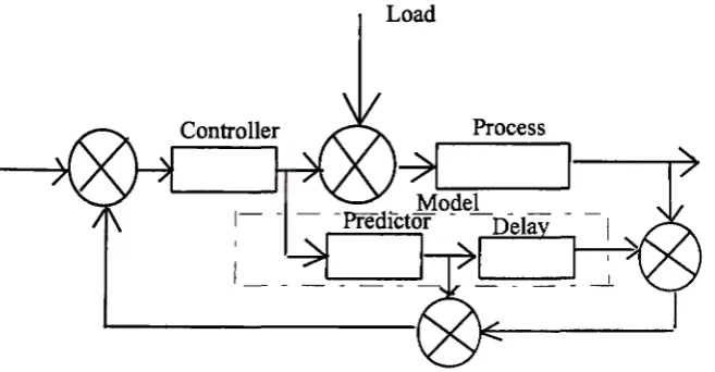
around it. Figure 1 gives a block diagram of the Smith predictor for dead-time

Load

Controller Process

Figure I Dead time compensation with Smith predictor

The Smith predictor contains two feedback loops; a positive loop containing

the dead time and a negative loop without it. The positive feedback loop is intended to

cancel the effect of the negative feedback loop through the process, leaving the

negative feedback loop in the predictor with only the lag and gain of the model in it.

This arrangement makes the predictor input identical to that which wpuld exist if there

were no dead time in the process, and hence results in better control. The

compensation technique involves the prediction of the process output through the use

of a process model which does not contain the dead time. The output of this predictor

element is also delayed with a time-delay element which constitutes a separate model

of the process dead time. With model dead time, lag and the controller gain matched

to a first-order process, the Smith predictor reproduces a step change exactly one dead

time later. For first-order processes, some form of derivative action is required, which

a Smith Predictor achieves in its feedback path. If the lag in the Smith Predictor is

matched to the lag (inertia) in a pure dead time process, the input manipulated

variable will follow the process lag exactly but delayed by the dead time. The delayed

predictor output is compared to the measured process output and the resulting model

deficiencies, provided that the model is a true representation of the process and if no

further disturbances enter dwing the dead-time period. In general, the optimal

predictor part of the controller algorithm will also change with the time delay. The

Smith predictor is an optimal dead-time compensator for only those systems having

disturbances for which the optimal prediction is a constant over the period of the dead

time.

In brief, the Dahlin's controller works on the principle proposed by Dahlin

[1968] that digital controllers be designed to yield a desired first order plus dead-time

response to a set-point or load change. Dahlin's algorithm specifies that the

sampled-data (discrete) closed-loop (feedback) control system behaves as though it were a

continuous first-order process with dead time. For designing sampled-data controllers,

Dahlin [1968] considered a tuning parameter ranging from 0 to 1 whereas in the

original formulation, the parameter could take values from -1 to 1. This dead time

compensator allows the use of a large process gain. To select a suitable value for the

Dahlin's tuning parameter, that is, the time constant of the closed-loop response, a

(trial or) initial value is assumed and the control system is simulated on a computer. A

proper selection of this parameter can be made by repeatedly varying this parameter

and examining the closed-loop response. The Dahlin computer-control algorithm is

designed for a specific input, for example, a step change in set point. If a load change

occurs in a process for which the control algorithm is based on a change in set point,

the response may not be equally good. The usual procedure, therefore, is to design for

the worst possible change in either set point or load that is likely to occur.

The dead time compensators are usually complex to deal with in real systems.

to that of a controller working on an unconstrained optimal control algorithm. The

precaution we have to take against instability for large gains in the real systems by

having a dead time compensator is by ensuring that there is no deviation between the

assumed dynamic (transfer function) model and the real system (Palmor and Shinnar

REFERENCES

(1)

(2)

Abraham, B., and Box, G.E.P., (1979), Sampling interval and feedback

control. Technometrics, 21 (no.1):1-8.

Astrom, K.J., and B.Wittenmark. (1984), Computer Controlled

Systems: Theory and Practice, Prentice-Hall, New Jersey.

(3) Baxley, Robert V. (1991), A Simulation Study Of Statistical Process

(4)

(5)

(6)

(7)

Control Algorithms For Drifting Processes, SPC in Manufacturing,

Marcel Dekker, Inc., New York and Basel.

Buckley, P.S. (1961), Automatic and Remote Control. (Edited by

Coales J.F.), Volume I, page 33. Butterworths, London. .

Box, G.E.P and Jenkins, G.M. (1970, 1976), Time Series Analysis:

Forecasting and Control. Holden-Day: San Francisco.

Chandra Prasad, C., and Krishnaswamy, P.R. (1975), Control of Pure

Time Delay Processes, Chemical Engineering Science, 1975, Volume

30, pages 207-215.

Dahlin, E.B., (1968), Designing and Choosing Digital controllers,

Instrumentation Control System. 4, 77.

(8) Harris, T.J., MacGregor, J.F. and Wright J.D. (1982), An Overview of

(9)

Discrete Stochastic Controllers: Generalized PID Algorithms with

Dead-Time Compensation, Can. J. Chem. Eng. 60, 425-432.

Harris, T.J., and MacGregor, J.F. ( 1987), Design of Discrete

Multivariable Linear Quadratic Controllers Using Transfer Functions,

(10) Kelly, S.J., MacGregor, J.F., and Hoffman, T.W., (1987), Control of a

Continuous Polybutadiene Polymerization Reactor Train, The

Canadian Journal of Chemical Engineering, Volume 65.

(11) Kramer, T.(1990), Process control from an economic point

ofview-lndustrial process control, technical report no.42 of the Centre for

Quality and Productivity Improvement, University of Wisconsin,

U.S.A.

(12) Kramer, T, (1990), Process control from an economic point

ofview-Dynamic adjustment and quadratic costs, technical report no.44 of the

centre for Quality and Productivity Improvement, University of

Wisconsin, U.S.A.

(13) MacGregor, J.F., (1976), Interfaces between process control and

on-line statistical process control, Computing and Systems Technology

division Communications, 10 (no.2): 9-20.

(14) MacGregor, J.F., (1988), On-line statistical process control, Chemical

Engineering Progress, 84, 21-31.

(15) Marshall, J.E., (1985), Control of time delay systems, Peter Peregrinus.

(16) Palmor Z.J. and Shinnar R., Design of Sampled Data Controllers,

(1979). Industrial and Engineering Chemistry Process Design

Development,Vol.18, No.1,8-30.

(17) Patranabis D., (1981), Tata McGraw-Hill Publishing Company

Limited, New Delhi.

(19) Smith, O.J.M. (1957) closer Control of Loops With Dead time, Chem.