A Study on Microstructures of Homogenization for Topology Optimization

(1)

A Study on Microstructures of

Homogenization for Topology

Optimization

By

Yulu Wang, BEngSc, MEngSc

A thesis submitted in fulfillment of the requirement of

the degree of Doctor of Philosophy

to Victoria University of Technology

School of Architectural, Civil and Mechanical Engineering

Victoria University of Technology

(2)

DECLARATION

This thesis does not contain any material, which has been previously submitted for a degree or diploma at any university. Except where due reference is made in the text, the work described in this thesis is the result of candidate’s own investigations.

_________________ Candidate

__________________ Supervisor

(3)

I wish to express my sincere gratitude to my supervisor, Dr. Danh Tran and co-supervisor, Prof. Mike Xie. They have been offering unfailing support in my PhD study. Their advice on technical matters, constant encouragement and motivation, ready accessibility and constructive criticism are greatly acknowledged. They made every effort to ensure that I was provided with excellent equipment and a comfortable working environment.

I would like to take this opportunity to express my appreciation to the School of Architectural, Civil and Mechanical Engineering, Victoria University of Technology which has provided research resources and facilities and a stimulating and positive study environment.

I am also grateful to the Victoria University of Technology in providing financial support through the Victoria University Postgraduate Research Scholarship, throughout my PhD study.

I wish to thank the academic and administrative staff of the School of Architectural, Civil and Mechanical Engineering for their encouragement, support and friendship throughout my study. I would also like to express my appreciation to the technical staff of the School in particular to Mr. Tien Do for their help.

(4)

This thesis studies topology optimization method employing the homogenization method, with a focus on different microstructures and their effects on the topology optimization solutions. The method is based on considering the design domain as a composite having an infinite number of infinitely small holes which are periodically distributed. As a result of introducing a material density function to represent the microstructure, the complex nature of the topology optimization problem can be converted to a problem of sizing optimization of determining the values of the parameters describing the microstructures. The main task for the homogenization method is to model and formulate these microstructures.

In the thesis, different microstructure models were investigated. The strengths and weaknesses of each type of microstructures were discussed. Homogenization method was employed to formulate the homogenized properties of the material. The optimality criteria and schemes of updating the design variables in the topology optimization process were derived for the newly developed microstructures and existing microstructures for which the information is not available in the literature. New microstructure models of one-material and bi-material were established. Based on these studies, a computer software package called Homogenization with Different

Microstructures (HDM) incorporating fifteen existing and the new

(5)

Firstly, the effects of the various one-material microstructure models were investigated. A number of examples of topological optimization problems with different loading cases were solved. The loading cases considered were single loading, surface loading, multiple loading and gravity loading.

For bi-material microstructure models, both cases of material without void and materials with void under different loading cases were studied. Benchmark topological optimization problems were investigated by using six different bi-material microstructure models that have been developed and programmed in the Chapter 4 and Chapter 5.

In the thesis, we proposed a new method to define microstructures to permit using shape optimization method to find optimal microstructures or using simple boundary shapes to describe a microstructure, hence to avoid the use of the complicated topology optimization method. Two types of microstructures, circular and cross shape were developed under this definition. Three multi-void microstructures and four new bi-material models are developed.

(6)

developed by Hassani and Hinton (1998).

(7)

____________________________________________________________ DECLARATION ii ACKNOWLEDGEMENTS iii

SUMMARY iv

TABLE OF CONTENTS vii

LIST OF FIGURES xii

LIST OF TABLES xix

NOTATIONS xx

CHAPTER 1 INTRODUCTION

1.1 General 1-1

1.2 Aims of the Research 1-4

1.3 Contribution of the Research 1-4

1.4 Significance of the Research 1-5

1.5 Layout of the Thesis 1-5

CHAPTER 2 OVERVIEW OF STRUCTURAL OPTIMIZATION

2.1 Structural Optimization Method 2-1

(8)

2.5.2 Topology optimization for continuous structures 2-16 2.6 Summary 2-18

CHAPTER 3 HOMOGENIZATION AND MICROSTRUCTURES REVIEW

3.1 Homogenization Method 3-2 3.1.1 Introduction 3-2 3.1.2 A brief review of periodic structure 3-4 3.1.3 The homogenization formulas in elastic composite materials with a

periodic structure 3-7 3.1.4 Application of homogenization for topology optimization in minimum

compliance problems 3-11

3.2 Microstructures Review 3-14

3.2.1 One-material microstructure 3-15 3.2.2 Bi-material microstructure 3-29 3.3 Summary 3-32

CHAPTER 4 MICROSTRUCTURES STUDY

4.1 Development of New Microstructures 4-1

4.1.1 Simple internal boundary (SIB) microstructures 4-2 4.1.2 Multi-void microstructures 4-8

4.1.3 Bi-material microstructures 4-9

(9)

4.2.2 Boundary condition 4-19 4.2.3 Computer Program Implementation 4-21

4.3 Summary 4-23

CHAPTER 5 OPTIMIZATION APPROACH

5.1 Optimality Conditions for Different Microstructure Models 5-2

5.1.1 Kuhn-Tucker conditions 5-4

5.1.2 Updating design variables 5-7 5.1.3 Optimality conditions for new microstructure models 5-9 5.1.4 Optimality conditions for existing microstructure models 5-21 5.2 Principal Stress Based Optimal Orientation 5-30 5.3 Convergence Criterion 5-31 5.4 Measures to Control Checkerboard Pattern 5-32

5.5 Computer Program Implementation 5-34

5.6 Summary 5-38

CHAPTER 6 COMPARISONS BETWEEN ALGORITHMS USING BENCHMARK TOPOLOGY OPTIMIZATION PROBLEMS 6.1 Algorithm Test by Deep Cantilever Beam Optimization 6-1 6.2 Comparing Algorithms for One-material Microstructure Models with

(10)

model 6-21 6.2.4 Iteration history for different material models 6-23

6.3 Comparisons Between Algorithms for Bi-material Microstructure

Models 6-26

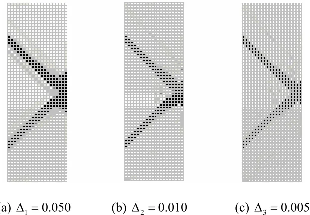
6.4 Effect of finite element discretization 6-34

6.5 Conclusions 6-36

CHAPTER 7 STUDY ON THE EFFECT OF VARIOUS ONE-MATERIAL MICROSTRUCTURES ON TOPOLOGY OPTIMIZATION RESULTS

7.1 Topology Optimizations with Single Load 7-2 7.2 Topology Optimizations with Surface Load 7-32 7.3 Topology Optimizations with Multiple Loads 7-53 7.4 Topology Optimizations with Gravity Load 7-57 7.5 Effect of Microstructures on Topology Optimization 7-60

7.6 Conclusions 7-62

CHAPTER 8 STUDY ON THE EFFECT OF BI-MATERIAL MICROSTRUCTURES ON TOPOLOGY OPTIMIZATION

8.1 Topology Optimization Using Bi-material Models with Void 8-2 8.2 Topology Optimization Using Bi-material Models without Void 8-14

8.3 Effects of Different Models on Topology Optimization 8-27

(11)

9.1 Conclusions 9-2 9.1.1 Comparison of microstructure models 9-2

9.1.2 Optimization results given by HDM 9-5

9.1.3 Optimal layout criteria 9-6

9.1.4 Checkerboard control 9-7

9.2 Recommendations for further investigations 9-7

Appendix A Appendix B Appendix C

(12)

Figure 2.1 Three categories of structural optimization 2-5

Figure 3.1 Homogenization limit 3-3

Figure 3.2 (a) A oscillating function 3-5

Figure 3.2 (b) One of oscillations in the expended scale 3-6 Figure 3.5 A periodic structure of composites and an enlargement of a

basic cell 3-6

Figure 3.4 A structure with cellar microstructures 3-8

Figure 3.5 A base cell 3-9

Figure 3.6 Ranked layered microstructure 3-16

Figure 3.7 Rectangular microstructure 3-20

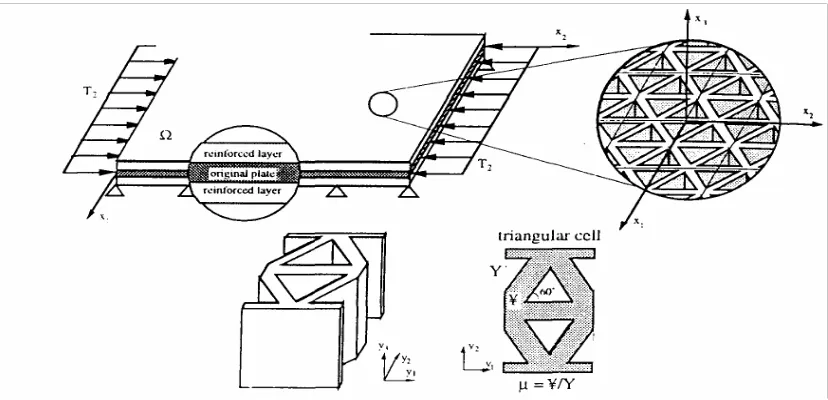
Figure 3.8 Triangular microstructure 3-22

Figure 3.9 Hexagon microstructure 3-23

Figure 3.10 Minimum weight microstructure 3-26

Figure 3.11 Four microstructures with extremal bulk modules 3-27 Figure 3.12 Topology optimized microstructures 3-28

Figure 3.13 Parameterized microstructures 3-29

Figure 3.14 Ranked layered bi-material cells 3-30

Figure 4.1 Definition of base cell 4-3

Figure 4.2 New coordinate system 4-3

Figure 4.3 A quarter of unit cell 4-3

(13)

model in 1 1

2 < ≤r 4-5

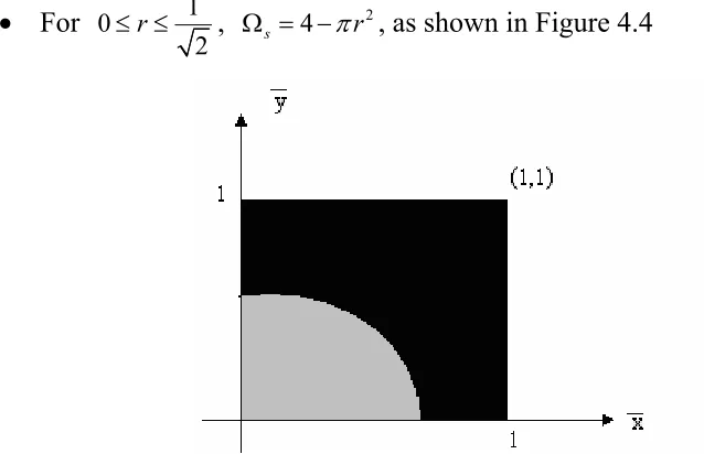
Figure 4.6 The area occupied by hard and soft materials of circular model for 1

2 r

0≤ ≤ −δ 4-6

Figure 4.7 The area occupied by hard and soft materials of circular

model for 1 1

2 r

δ _δ

−

< ≤ − 4-6

Figure 4.8 The area occupied by hard and soft materials of circular

model for 1− < ≤δ r 1 4-7

Figure 4.9 Cross shape boundary 4-8

Figure 4.10 Multi-void microstructures 4-9

Figure 4.11 Bi-material microstructures 4-10

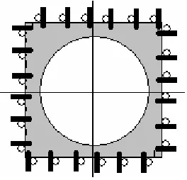
Figure 4.12 Boundary conditions for case a, b and c 4-20

Figure 4.13 Boundary conditions for case d 4-21

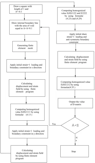
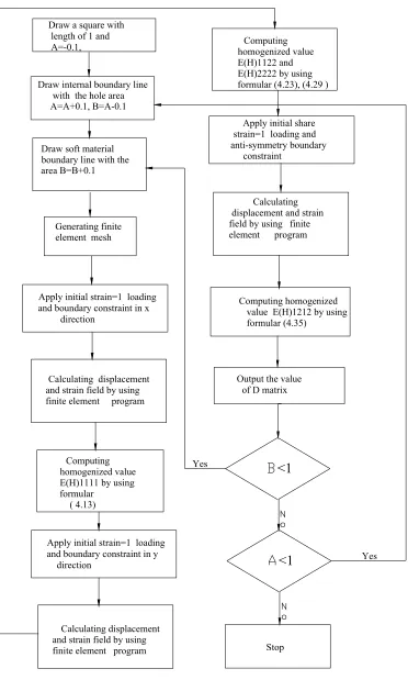
Figure 4.14 Algorithm for one-material model 4-23 Figure 4.15 Algorithm for bi-material model 4-24 Figure 4.16 Polynomials for cross shape model 4-25 Figure 5.1 Geometrical interpretation of Kuhn-Tucker condition 5-5

Figure 5.2 Checkerboard problem 5-32

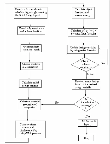
Figure 5.3 Topology optimization procedure using homogenization

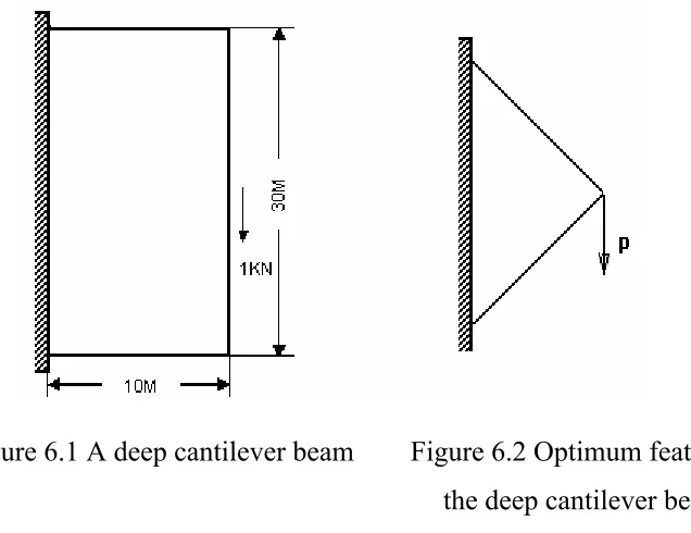
method 5-40 Figure 6.1 A deep cantilever beam 6-2

(14)

Figure 6.4 Optimum layout of deep cantilever beam for ranked

layered material model 6-3

Figure 6.5 Optimum layout of deep cantilever beam for triangular

material model 6-4

Figure 6.6 Optimum layout of deep cantilever beam for hexagon

material model 6-4

Figure 6.7 Optimum layout of deep cantilever beam for cross shape

material model 6-4

Figure 6.8 Optimum layout of deep cantilever beam for circular

material model 6-5

Figure 6.9 Optimum layout of deep cantilever beam for triangular

multi-void material model 6-5

Figure 6.10 Optimum layout of deep cantilever beam for rectangular

Figure 6.11 Optimum layout of deep cantilever beam for square

Figure 6.12 Optimization layouts of case a 6-8~10

Figure 6.13 Optimization layouts of case b 6-11~13

Figure 6.14 A short cantilever beam 6-15

Figure 6.15 Discretized design domain from Min etc. 6-15 Figure 6.16 Optimal structure layouts from Min etc. 6-16 Figure 6.17 Convergence histories in the case of volume constraint

(15)

Hinton 6-17 Figure 6.19 Optimal layouts of using artificial model with different

penalty from Hassani and Hinton 6-18

Figure 6.20 The iteration history of using artificial model with

different penalty from Hassani and Hinton 6-18 Figure 6.21 The optimization results of using ranked layered material

model from Hassani and Hinton 6-18

Figure 6.22 The iteration history of using ranked layered model from

Hassani and Hinton 6-19

Figure 6.23 Optimization result with different microstructures 6-20~21 Figure 6.24 Optimization results for different power values 6-22~23 Figure 6.25 Iteration histories for different material models 6-24~25 Figure 6.26 Iteration histories for different power values 6-27~28

Figure 6.27 A cantilever beam problem 6-29

Figure 6.28 Optimal layout from Thomsen 6-30

Figure 6.29 Optimization layouts of using HDM 6-31~33 Figure 6.30 The optimum layouts for different finite element

discretizations. 6-34 Figure 6.31 Iteration histories for different finite element

discretizations. 6-35

Figure 7.1 A simply supported beam 7-3

(16)

HDM for the simply supported beam problem 7-3~5 Figure 7.4 Iteration histories with different models for the simply

supported beam problem 7-7~8

Figure 7.5 Comparison iteration histories 7-9 Figure 7.6 Optimization results with different power values for the

simply supported beam optimization 7-10~12 Figure 7.7 Iteration histories with different power values for the

simply supported beam problem 7-13~14

Figure 7.8 A square domain with a point load 7-16 Figure 7.9 Optimum layouts of using the PLATO software for the

square domain with a point load problem 7-17 Figure 7.10 Optimization result for different microstructures for

case a 7-17~19

Figure 7.11 Optimum layout of using PLATO with rectangular

model 7-20 Figure 7.12 Optimization layouts for different models for case b 7-20~21

Figure 7.13 Optimization results with different power values for the

volume fraction Vs / V = 40%. 7-22~23

Figure 7.14 A domain with two sides’ boundary constraints 7-24 Figure 7.15 Optimum layout of using PLATO software for the domain

with two sides’ boundary constraints problem 7-25 Figure 7.16 Optimization layouts of different microstructures for the

(17)

the two sides’ boundary constraints problem 7-29~32 Figure 7.18 Design domain of a bridge model 7-33 Figure 7.19 Result of using PLATO software for the bridge model 7-33 Figure 7.20 Optimization layouts of different microstructures for the

bridge model 7-34~36

Figure 7.21 Sydney Harbor Bridge 7-36

Figure 7.22 Iteration histories of different material models for the

bridge model problem 7-37~38

Figure 7.23 Optimization layouts of different power values for the

Figure 7.24 Iteration histories of different power values for the

Figure 7.25 A square domain with pressure load 7-46 Figure 7.26 Result of using PLATO software for the square domain

with pressure load problem 7-46

Figure 7.27 Optimization layouts of different microstructures for the

square domain with pressure load problem 7-47~48 Figure 7.28 Optimization results with different power values for the

square domain with pressure load problem 7-49~50 Figure 7.29 Optimization layouts of different microstructures for the square

(18)

simply supported beam with multiple load 7-54~56 Figure 7.32 Design domain under gravity loads 7-57 Figure 7.33 Optimization layouts for different microstructures

models with gravity load 7-58~59

Figure 8.1 Optimization layouts of bi-material models 8-3~4 Figure 8.2 Iteration history for ranked layered bi-material model 8-4 Figure 8.3 Iteration histories for the rest of bi-material models 8-5 Figure 8.4 Optimization layouts for different power values 8-6~7 Figure 8.5 Layouts of six bi-material models 8-7~8 Figure 8.6 Result layouts of six bi-material models 8-10~11 Figure 8.7 Design domain of a bridge model 8-12 Figure 8.8 Optimization layouts of six bi-material models 8-12~13

Figure 8.9 A short cantilever beam 8-15

Figure 8.10 Result layouts of six bi-material models 8-15~17

Figure 8.11 A supported beam 8-18

Figure 8.12 Optimization layouts of six bi-material models 8-18~19

Figure 8.13 A two side’s supported beam 8-20

Figure 8.14 Optimization layouts of six bi-material models 8-20~22

Figure 8.15 Press machine frame model 8-23

(19)

Table 4.1 Parameters of the bi-material models 4-10 Table 6.1 Iteration numbers for different convergence tolerance 6-6

Table 6.2 The initial and final strain energy for different power values

for short cantilever beam problem 6-28

Table 6.3 Strain energies for the different finite element discretizations 6-35 Table 7.1 Iteration numbers and final strain energies at convergence

tolerance for the microstructures using HDM 7-9 Table 7.2 The initial and final strain energy with different power values for

single supported beam optimization 7-15 Table 7.3 Iteration numbers and final strain energies at convergence

tolerance for the microstructures using HDM 7-39 Table 7.4 The initial and final strain energy for different power values for the

bridge model problem 7-44

Table 8.1 Iteration numbers and final strain energies at convergence tolerance

for the microstructures using HDM 8-5

Table 8.2 Iteration numbers and final strain energies at convergence tolerance

(20)

NOTATIONS

________________________________________________________________

Acronyms:

CATO Constrained adaptive topology optimization software developed by Bulman, Sienz and Hinton.

ESO Evolutionary structural optimization

HDM Homogenization with different microstructures program

PLATO Topology optimization software developed by Hassani and Hinton SIB Simple internal boundary

SIMP Solid Isotropic Microstructures with Penalization

Strand7 Finite element software developed by G+D Computing Limlted

Tensors, Scalars and Functions

( , )

a u v Energy bilinear form for internal work a Design variables

b Design variables

e as a superscript indicates dependency to the cell of periodicity f(x) Objective function

f Average body forces within the cell

k

(21)

p Function of the position vector x q Function of the position vector x r Design variable

s Boundary of the hole in base cell t Slack variables

1 i

u% Arbitrary constants of integration in y

i

u Displacement associate with i

l m

x Lower bounds of design variable

u m

x Upper bounds of design variable ,

x y Global Cartesian coordinates

i

x , y_i Cartesian coordinate of node i E Young’s modulus of solid material

ad

E Admissible elasticity tensors

ijkl

E Elasticity tensor

G ijkl

E General elasticity tensor

H ijkl

E Homogenized elasticity tensor

e ijkl

E Coefficients of elasticity of an inhomogeneous body F Objective function

G Base cell body H Hole of the base cell

(22)

2

L Hilbert space

L Lagrangian function

g

N Global shape function.

i

Y Dimension of periodic base cell

Greek symbols

α Solid part shape function β Y- periodic function ζ Lagrangian multiplier

ij

δ Kronecker delta symbol

λ Lagrangian multiplier

ij

ε Second order strain

0

ε Initial strain loading

δ A small value to define solid size

ς Small parameter indicating the characteristic of non-homogeneity dimension

ij

σ Second order stress

ij

σ Average residual stress within the cell

θ Orientation angle

µ Intermediate values as a penalization

(23)

η Moving limit

ρ Density

)

χ Discrete function ( )χ _kl Y- Periodic function ∆ Convergence tolerance

( )x

ξ Continuous approximation function Ψ Solid part of cell

Π Total potential energy Ω Design domain

s

Ω Solid part of design domain

t

Γ Boundary on which the surface force applied

d

Γ Boundary on which displacements are prescribed

Special Symbols

g Norm

∈ Belongs to

∑

Summation

∩ Intersection of sets

∀ For all

(24)

f Vector of structure load

p Vector of surface force in the hole

t Vector of traction force u Displacement vector

v Vector of virtual displacement x Vector of design variables

y Position vector in microscopic coordinate

p

Y Vector of periodicity, Yp = Y Y Y_{1, 2}, ₃T

e i

f Force vector for element e associated with node i

n

R n dimensional space

V Space of admissible displacement

Ω×Ψ

V Space of admissible displacements defined in Ω× Ψ ( )Y

W Space of periodic function B Strain-displacement matrix D Element of constitutive matrix

G

D Element of general constitutive matrix of

H

D Element of homogenized constitutive matrix K Symmetric, banded stiffness matrix

N Matrix of arbitrary integers

1 2

3

0 0

n n

n

 

 

=  

 

 

N

(25)

Chapter 1 INTRODUCTION

1.1 General

The natural resources available to human beings are very limited, which means

we should use these resources as efficiently as possible. Optimization is a tool

for finding the best possible solution to an engineering problem. In this

respect, optimization plays a very important role in the engineering field.

The concept of an optimum in an engineering problem is intriguing and has

been under intensive investigation for decades. Earlier, engineering design was

conceived as a kind of art that demanded great ingenuity and experience of the

designer, and the development of the field was characterised by gradual

improvement of existing types of engineering design. The design process was a

sequential trial and error. It started from an initial design based on the

knowledge and experience of the designer, then followed by an analysis to the

performance of the design. Based on the information obtained, a new design

was developed. Nowadays, intense technological competition requires

(26)

and functionality. The current concept of design places greater emphasis on

efficient use of energy, environmental problems, saving as much natural

resources as possible, Therefore it often involves creative activity for which

prior engineering experience is totally lacking. Such creativity must naturally

resorts to application of scientific methods. In recent decades, the development

of computer technology has provided the opportunity to revolutionize the

traditional design process. The engineering design has been changing from trial

and error to scientifically based methods of rational design and optimization.

This has already occurred with structural optimization.

Structural optimization is a part of an optimal design field dealing with

structural elements or structural systems and is employed in several

engineering fields. The main task of structural optimization is to find the ‘best

possible solution’ to a structure that meets all the multidisciplinary

requirements imposed by functionality and manufacturing conditions. A

structural optimization design is a rational establishment of a structure which is

the best of all possible solutions within a prescribed objective and a set of

constraints. Structural optimization has become a multidisciplinary subject with

applications in many fields, such as automotive, aeronautical, mechanical, civil,

nuclear, naval and off-shore engineering. As a result of rapidly growing

applications of structural optimization, the importance of the research in

structural optimization methods is realized by more and more scientists and

(27)

Topological structural optimization is regarded as one of the most challenging

topics in structural mechanics, in which one needs to change the topology as

well as the shape during the process of optimization. This significantly

increases the complexity of the optimization problem.

In order to overcome the difficulty of topology optimization problems, various

optimization design techniques have been developed in recent decades. Among

these, the homogenization method proves to be one of the general approaches

to shape and topology optimization. This method is based on the theory of

homogenization. The main idea of the homogenization method is to consider

the design domain as a composite material consisting of an infinite number of

periodically distributed small holes. By introducing a material density function,

the complex nature of the topological optimization problem can be converted to

a sizing optimization problem by treating the sizes of the small holes as the

design variables. The very important task of homogenization method for

topology optimization is to create and formulate a microstructure model for the

design domain.

Although there has been considerable work done in the field of the

homogenization method for structural topology optimization, the studies and

comparisons of the existing microstructures and exploration for new

microstructures are comparatively modest and limited. More studies on

(28)

1.2 Aim of the Research

The general aim of the research is to develop simple, general, and more

computationally efficient microstructures to improve the homogenization

method so that it can be put for practical use and to examine the effect of these

different microstructures on different kinds of topology optimization problems.

The specific aims of the proposed project are:

a. Investigating the properties of existing microstructures.

b. Identifying the strengths and weaknesses of each type of microstructures.

c. Establishing new microstructures for shape and topology optimization.

d. Deriving an efficient algorithm of optimization procedure for different

microstructure models.

e. Developing a general computer software package incorporating all the

existing and new microstructures.

f. Solving different types of optimization problems by using different

microstructures and comparing the optimization results.

1.3 Contribution of the Research

In this thesis, a study on the microstructures has been carried out and new

microstructures including one-material and bi-material microstructures have

been proposed. These microstructures help to overcome the inherent difficulties

(29)

design more accurate. A computer software package for topology optimization

catering for all microstructures, existing and newly studied here, was developed.

All these will reduce the gap between the mathematical complexity of

topological optimization and its practical application in engineering design.

1.4 Significance of the Research

In the topology optimization field, the homogenization method can be used to

solve a wide range of practical problems. In this respect, this study is

significant in that it contributes to the development of homogenization to a

comprehensive and practical tool in engineering. The finding from this research

will provide useful information for researchers and design engineers in

choosing microstructures suitable for their tasks. The computer software

package can be used for practical applications as well as for future research and

development. Consequently, more efficient designs using less material and

energy can be obtained for engineering structures.

1.5 Layout of the Thesis

The thesis consists of nine chapters. An outline is given as follows:

Chapter 1 outlines the general background and basic concept of structural

optimization and the homogenization method as well as the aims, contribution

(30)

Chapter 2 presents a comprehensive review of the development history and

status of structural optimization. Different optimization methods are described

and their advantages and limitations are discussed, topological optimization

methods are emphasized.

Chapter 3 describes the theoretical basis of the homogenization method and its

application in topological optimization. In this chapter, the concept of periodic

structure is first described. It is followed by the homogenization formulas in

elastic composite materials with a periodic structure and the application of

homogenization method in topology optimization. Next is a review on

microstructures. In this section, different models of microstructures are studied.

The advantages and disadvantages of current microstructures model are

described. Finally, a brief summary is presented.

Chapter 4 In this chapter, a new definition for developing microstructures is

given. Nine new microstructure models are developed. The method for

deriving material properties of the new microstructures is studied.

Chapter 5 mainly deals with computer program implementation for different

microstructure models, followed by the treatment of the technique of

principal-stress based optimal orientation and checkerboard control technique.

Chapter 6 In this chapter, structural topology optimization of a number of

(31)

are tested and compared with other methods.

Chapter 7 deals with different loading cases (single load, surface load,

multiple load, and gravity load cases). A series of structural topological

optimization problems are carried out. The results and their accuracy for

different microstructures are compared. Advantages and disadvantages of

different microstructures are summarized.

Chapter 8 conducts numerical tests on bi-material models. The two types

investigated are: one is a model of bi-material without void and the other is

bi-material with void. Examples of structural topological optimization under

different loading cases are presented. Their solutions are compared. Advantages

and disadvantages of different bi-material microstructures are summarized.

Chapter 9 presents general conclusions regarding the effectiveness and

efficiency of microstructures studied. Suggestions for further investigations

were given.

Appendix A presents the homogenization formulas in elastic composite

materials with a periodic structure.

Appendix B presents a typical run of the HDM software.

Appendix C presents Optimality criteria for deep cantilever beam with a single

load

(32)

Chapter 2

_________________________________________________________

OVERVIEW OF STRUCTURAL OPTIMIZATION

This chapter reviews the development of the theory of structural optimization

and its applications. The background of structural optimization method is first

described, followed by mathematical description for general optimization

problems. Approaches for structural optimization including classical calculus

methods and numerical methods are reviewed and their algorithms are

presented. Topology optimization is introduced in more details. The current

situation and future directions of structural optimization are summarized.

2.1 Structural Optimization Method

A structural optimization design problem is described by the objectives of the

problem, the constraints involved and the design variables. A general structural

optimization problem is formulated as: “Minimise (or maximise) an objective

function subject to behavioural and geometrical constraints.”

The objective function or behavioral constraints are usually described as

(33)

• structural volume or weight, storage capacity.

• cost of material or manufacturing.

• global measure of the structural performance such as stiffness, buckling

load, plastic collapse load, natural vibration frequency, dynamic

response, etc.

• local structural responses such as stress, strain or displacement at

prescribed points; maximum stress, strain or displacement in the whole

structure, stress intensity factor, etc.

Geometrical constraints are usually described as follows:

• manufacturing limitations.

• availability of member sizes.

• fabrication.

• physical limitations.

The design variables are to be determined during the optimization process.

Design variables can be continuous or discrete.

2.2 Mathematical Description of an Optimization Problem

An optimization problem can be mathematically stated as searching for the

minimum (or maximum) value of a function f( )x and the related variable vector ( , ... )₁ ₂ n, is n dimensional space, which yields the optimal

n x x x =

(34)

solution subject to some constraints. The optimization problem in its most

general form may be expressed as follows (Haftka and Gurdal, 1992):

( )

( ) 0 1, 2, , ( ) 0 k 1, 2, ,

j

k k

Minimize f

Such that h j n

g n

= =

≤ =

x x

x

ggg ggg

h (2.1)

where and are constraints, j and k are the number of equality of

constraints and inequality constraints, respectively. j

h g_k

The sets of design variables which satisfy all the constraints constitute the

feasible domain. The infeasible domain is the collection of all design points

that violate at least one of the constraints. If the objective function and both

equality and inequality constraints are linear functions of the design variables,

then the problem is a linear optimization problem. In a non-linear optimization

problem, either the objective function or at least one of the constraints is a

non-linear function of the design variables. From the engineering point of view, the

objective function f(x) is usually chosen as the structural volume, weight, cost, performance, serviceability or their combination. Structural optimization

problems are usually non-linear optimization problems (Chu, 1997).

2.3 Classifications of Structural Optimization

According to the design variables to be optimised, the structural optimization in

(35)

Sizing optimization: In this type of optimization problems, the domain of the structure is fixed during the optimization process. Design variables for sizing

can be discrete or continuous. Sizing optimization can usually be considered as

the implementation of optimization at details design stage.

Shape optimization: In shape optimization problems, the domain is not fixed but the topology is. Shape optimization is always used in the selection of the

optimum shape of external boundary surfaces or curve. Examples of this type

of problem include finding the boundaries of a structure, finding the location of

joints of a skeletal structure, finding the optimal values for parameters, which

define the middle surface of a shell structure. This may be seen as the

implementation of the optimization techniques at the preliminary design stage.

Topology optimization: In some cases, sizing and shape optimization methods may lead to sub-optimal results. To overcome this deficiency topology

optimization must be considered. Topology optimization is to find the optimal

layout of a structure within a defined design domain. Different from shape or

sizing optimization method, the initial design domain in topology optimization

is a grand or universal structural, for example, a rectangular plate, in some two

dimensional design problems. The only known quantities in the problem are the

applied loads, the possible support conditions, the volume of the structure to be

constructed and maybe some additional design restrictions defined by the

designer. The physical size, shape, and connectivity of the structure are not

(36)

standard parametric functions but by a set of distributed functions defined over

the fixed design domain. These functions in turn represent a parameterization

of the stiffness tensor of the continuum and a suitable choice of this

parameterization, which would lead to the proper design formulation for

topology optimization (Bendsøe and Sigmund, 2002). Topology optimization

is the most difficult and challenging task among the three types of structural

optimization problems.

Figure 2.1, which is extracted from Bendsøe and Sigmund (2002) shows the

three categories of structural optimization, a) sizing optimization problem of a

truss structure, b) shape optimization and c) topology structural optimization.

Figure 2.1 Three categories of structural optimization.

(From Bendsøe and Sigmund, 2002, page 2)

2.4 Solution Methods for Structural Optimization

Different approaches to solve the structural optimization problems can be

(37)

2.4.1 Calculus methods

The differential calculus was introduced into optimization problem in the 17th

century. The first use of the calculus methods to structural design can be

attributed to Maxwell (1895) in designing the least weight layout of

frameworks. The later research on the optimal topology of trusses by Michell

(1904) resulted in the well known Michell type structures. The typical calculus

methods are differential calculus and calculus of variations

Differential Calculus

The method of differential calculus stated that the conditions for existence of

extreme values are the first order partial derivatives of the objective function

with respect to the design variable to be zero.

The formula of differential calculus is as follows:

( ) 0,_i 1, 2,...., .

F x i n

∇ = = (2.2)

Where the vectorx= {xl, x2,..., xn} is the extreme points.

The differential calculus usually can only be applied to very simple cases such

as unconstrained optimization problems.

Calculus of Variations

Calculus of variations is a generalization of the differentiation theory. It deals

(38)

definite integral of a functional Q, Q is defined by an unknown function y and

some of its derivatives (Haftka and Gurdal 1992):

( , ,..., )

b n

n a

d d

F Q d

d d

=

_∫

x, y y y x

x x (2.3)

Where y y(x)= is directly related to the design variable x. Optimization is to find the form of function y y(x)=

instead of individual extreme values of

design variables.

The necessary condition for an extremum is the first order of variation equal to

zero.

( ' ...) 0

' b

a

Q Q

F

δ = ∂ δ +∂ δ + d

∂ ∂

∫

y y x

y y = (2.4) Where y'=dy/dx

Taking into account of boundary conditions at fixed y(a) and y(b) (Haftka and Gurdal 1992), Equation (2.4) can be expressed as

0 '

Q d Q

d

 

∂ ∂

− _ _

∂y x_∂y _= (2.5) This is the well known Euler-Lagrange equation.

Although the application of calculus method is very limited, it is a very

important stage in the development of optimization methods. Calculus methods

have the fundamental importance in exploring mathematical nature of

optimization and in providing the lower bound optimum against which the

(39)

2.4.2 Numerical methods

In general structural optimization problems are highly non-linear. In the design

of real structural systems, the use of numerical methods is unavoidable.

Nowadays the numerical methods of structural optimization generally fall into

the following categories:

• Direct minimization techniques (e.g. mathematical programming, MP)

• Indirect methods (e.g. optimality criteria, OC)

• Genetic Algorithms method

Mathematical Programming

Mathematical programming (MP) was one of the most popular optimum search

techniques formulated in 1950s (Heyman 1951). It is a step-by-step search

approach involving iterative processes. Each iteration consists of two basic

steps:

a) differentiating the value of the objective function and its gradients with

respect to all design variables,

b) calculation of a change of the design variable that would result in a

reduction of the objective function.

Steps a) and b) are repeated until a local minimum of the objective function is

(40)

In the early stages, the mathematical programming method was only limited to

linear problems where the objective functions and constraints are linear

functions of design variables. Since 1960, numerous algorithms of nonlinear

programming techniques have been developed such as: nonlinear programming

(NLP) (Schmit, 1960), feasible direction (Zoutendijk 1960), gradient projection

(Rosen 1961) and penalty function method (Fiacco and McCormick 1968). At

the same time, approximation techniques using the standard linear

programming to address nonlinear problems, such as sequential linear

programming (Arora 1993) have been studied.

The main advantage of MP methods is that they can be applied to most

problems within and outside the field of structural optimization. The main

disadvantage of MP methods is that as the number of design variables and

constraints increases, the cost of computing derivatives becomes expensive.

Optimality Criteria

Optimality criteria are necessary conditions for minimality of the objective

function and these can be derived by using either variational methods or

extremum principles of mechanics. Optimality criteria (OC) method was

analytically formulated by Prager and co-workers in 1960s (Prager and Shield

1968; Prager and Taylor 1968). It was later developed numerically and become

(41)

OC methods can be divided into two types. One type is rigorous mathematical

statements such as the Kuhn-Tucker conditions. The other is algorithms used to

resize the structure for satisfying the optimality criterion. Different

optimization problems require different forms of the optimality criterion.

In Kuhn-Tucker conditions (Haftka and Gurdal 1992), the inequality

constraints can be transformed into equality constraints by adding slack

variables. In this case, the inequality constraints in Equation (2.1) can be

written as

2 k

t is slack variables

2

( ) 0, 1, 2,3, ,

k k

g x + =t k= ⋅⋅⋅ n_g (2.6)

The Lagrangian function of the optimization can be defined as

2 (2.7)

1 1

( , , , ) ( ) ( ) ( ( ) )

g

h n

n

j j k k k

j k

L t λ ζ f ζ h λ g t

= =

= +

∑

+

∑

+

x x x x

where ζ_j and λ_k are Lagrangian multipliers.

Differentiating the Lagrangian function (2.7) with respect to x, t, λ, and ζ_j we obtain

1 1

( ) ( )

0, 1, 2, , g h n n j k j k j k

i i i i

h x g x

L f

i

x x = ζ x = λ x

∂ ₌ ∂ ₊ ₊ ₌ ₌ _⋅⋅⋅

∂ ∂

∑

∂

∑

∂ n (2.8)

0 1, 2, ,

j h j L h j ζ ∂ ₌ ₌ ₌ _⋅⋅⋅

∂ n (2.9)

2 ₀ _{1, 2, ,} k k

k L

g t k n

λ

∂ ₌ _{+ =} ₌ _⋅⋅⋅

(42)

2 _{k k} 0 1, 2, , _g k L t k t λ ∂ ₌ ₌ ₌ _⋅⋅⋅ ∂ n n (2.11)

From (2.10) and (2.11) we can get

( ) 0, 1, 2, , 0, 1, 2, ,

k g

k k g

g x k n

g k

λ

≤ = ⋅⋅⋅

= = ⋅⋅⋅ (2.12)

This implies that when an inequality constraint is not active, the Lagrangian

multiplier associated with the constraint is zero.

By using Kuhn-Tucker conditions, the optimality conditions for the

optimization problem can be stated as

1 1

( ) _{( )}

0, 1, 2, , 0 1, 2, , ( ) 0,

g h n n j k j k j k

i i i i

j h

j k

h x _{g x} L f

i n

x x x x

L h j g x ζ λ ζ = = ∂ ∂ n = + + = = ∂ ∂ ∂ ∂ ∂ ⋅⋅⋅ = = = ⋅⋅⋅ ∂ ≤

∑

1, 2, , 0, 1, 2, , 0, 1, 2, ,

g

k k g

k g k g k k n λ λ n n = ⋅⋅⋅ = = ⋅⋅⋅ ≥ = ⋅⋅⋅ (2.13)

The optimal criteria method is one of the best-established and widely accepted

optimization techniques.

It should be mentioned here the attempt to combine both the mathematical

(43)

dual methods search the optimum direction in the space of Lagrangian

multipliers instead of that of the initial design variables, it can save

considerable computing efforts when the number of constraints is smaller than

that of design variables (Fleury, 1979).

Genetic Algorithms

Genetic Algorithms (GA) were first developed in 1970s (Holland, 1975). The

GA method uses genetic processes of reproduction, crossover and mutation.

The procedures are summarized as follows:

a) An initial population of designs is randomly created.

b) The fitness of each individual is evaluated according to a fitness

function.

c) The fittest members are reproduced and allowed to cross among

themselves.

d) A new generation is developed with member having higher degree of

desirable characteristics than the parent generation.

e) This procedure is repeated until a near optimum solution has been

reached.

Although the GA method may not yet be as popular as MP or OC method, this

method has merits of being reliable and robust (Nagendra, Haftka and Gurdal,

(44)

2.5 Structural Topological Optimization

With the exception of a few early landmark results (Maxwell 1895; Michell

1904), the historical development of the field of structural optimization seems

to have followed an opposite route to the actual structural design process

(Haftka and Gurdal 1992; Kirsch 1993). Since its inception, research in

numerical optimal structural design went from element stiffness design,

through geometric and shape optimization to topology optimization design. It is

also clear that the major impact on the structural efficiency, in the sense of

stiffness/volume or stress/volume ratio, is determined at the conceptual stage

by the topology and shape of the structure. No amount of fine-tuning of the

cross-sections and thicknesses of the elements will compensate for a conceptual

error in the topology or the structural shape (Olhoff et al. 1991).

With the development of high-speed computer, the topology optimization

method using numerical approach has been growing quickly (Haftka and

Grandhi (1986), Kirsch (1989) and Rozvany et al. (1995)). A numerical

approach to topological design starts with a domain of material to which the

external loads and boundary conditions apply. The optimization algorithm then

proceeds with removing out ineffectual material to generate best structural

solutions. In most cases, the objective function for topology optimization

(45)

Generally speaking, structural topology optimization can be considered as a

material distribution problem. Two classes of structural domains have been

used in topology optimization problems. One is called the ‘Discrete’ structure.

Early solutions can be seen in the papers of Don et al. (1964); Dobbs and

Felton (1969), examples of applying the concept to large-scale structures have

been given by Zhou and Rozvany (1991). The other domain is continuous

structures. The continuum is typically divided into appropriate finite elements

where every element has intrinsic structural properties. They are reviewed in

the following sections.

2.5.1 Topology optimization for discrete structures

According to the survey by Topping (Topping, 1993), topology optimization

method for discrete structures can be classified into three categories:

Geometric Approach

In the geometric approach, the properties of cross-section and the coordinates

of joints are design variables. During the optimization process, the number of

joints and connecting members are fixed while some joints are permitted to

coalesce.

Hybrid Approach

In the hybrid approach, the design variables are divided into size design

(46)

space. During the optimization process, the element size is firstly changed

while keeping the topology unchanged; next, optimum position of the element

nodes is searched.

Ground Structure Approach Method

Combined with the MP and OC method, the ground approach method is now

widely used in topology optimization problems. In the ground structure

approach, a ground structure is considered as a dense set of nodes and a

number of potential connections between the nodes. During the optimization

process, the number and size of connecting elements are changed, but the nodes

numbers and position are fixed. If the section area of elements are reduced to

zero during the optimization process, the elements are considered as

non-existent and the topology is changed accordingly.

A remarkable advantage of the ground structure approach method is that the

design domain is fixed thus the problem of mesh regeneration can be avoided.

2.5.2 Topology optimization for continuous structures

Heuristic Methods

Heuristic methods are those addressing structural optimization problems in a

(47)

formulation, the heuristic methods are based on simple concepts or natural

laws. These methods fall into two categories.

Evolutionary structural method (ESO)

The evolutionary structural method was first proposed by Xie and Steven

(1993, 1994a). This method is based on the concept of slowly removing the

inefficient material from the structure and/or gradually shifting the material

from the strongest part of the structure to the weakest part until the structure

evolves to the desired optimum. The ESO method offers a simple way to obtain

optimum designs using standard finite element analysis codes. Compared to

other structural optimisation methods, the ESO method is overwhelmingly

attractive due to its simplicity and effectiveness. During the last ten years, ESO

has been demonstrated to be capable of solving many problems of size, shape

and topology optimum designs for static and dynamic problems (Rong et al,

2001).

Homogenisation Method

Compared to the methods discussed above, the homogenization method is more

complex. This method is based on the mathematical theory of homogenization,

which has been developed since 1970’s (Babuska, 1976, Cioranescu and Paulin

1979). The homogenization method can be used to find the effective properties

of the equivalent homogenized material and can be applied to many areas of

(48)

in 1988 by Bendsøe and Kikuchi (1988), homogenization method has attracted the attention of many researchers and design engineers and has been used by

industrial companies around the world for product development, particularly in

the automobile industry.

The homogenisation method has been successfully applied to both static and

dynamic problems with weight constraint (Tenek and Hagiwara 1993, Ma et al.

1995). With regard to the algorithm aspect, the homogenisation method uses

traditional mathematical programming or optimality criteria as search

techniques. The advantages of homogenization method are rigorous theoretical

basis and good convergence behaviour. The disadvantage of homogenization

method is that difficulties associated with those traditional methods are

magnified in the homogenisation method.

H/e-method

The h/e-method is a hybrid method. It is an abbreviation of the combination of

homogenization and evolutionary methods in various degrees. Bulman, Sienz

and Hinton (2001) developed the CATO (constrained adaptive topology

optimization) algorithm combines idea from the two procedures: the more

mathematically rigorous homogenization method and more intuitive

evolutionary methods. They systematically investigated the performance of the

algorithm for topology optimization using a series of benchmark problems and

their study results show that in general cases, the h/e CATO algorithms

(49)

2.6 Summary

With the development of computer technology, structural optimization has

become a very important design tool in engineering. The applications of

structural optimization designs have been widely extended to various fields

such as aerospace, transportation, mechanical and civil engineering.

Numerical methods have been developed very rapidly and have been widely

used in the structural optimization problems. With the advance of high-speed

computers and the relatively inexpensive computational power, numerical

methods play more and more important role in structural optimization.

In structural optimization problems, topological structural optimization has the

complex features of both sizing, and shape optimization problems. In the

optimization process, trying to change the topology as well as the shape during

the optimization processes makes the problem more complex. This class of

problems is still regarded as one of the most challenging in structural

mechanics.

Homogenization method is very useful tool in solving topology structural

optimization problems. It is regarded as the one of the most general approach to

finding optimum shapes and topology of structures. Details of this method will

(50)

Chapter 3

_________________________________________________________

HOMOGENIZATION AND MICROSTRUCTURES

REVIEW

By using the concept of the composite microstructures distribution, the

homogenization method can be used to solve structural topology optimization

problems. The results obtained have good agreements with the experimental

data available in literature.

In general, the mathematical theory of homogenization does not provide

analytical formulas or numerical algorithms directly suited to obtaining

answers to engineering problems. Thus, a 'gap' exists between the mathematical

theory of homogenization and the mechanics of composites. This gap acts as

the principal obstacle to a wide application of the methods of the mathematical

theory of homogenization in practical work. To solve this problem,

microstructure model of homogenization and its formulation must be well

established.

In the last ten years, researchers and engineers have done a lot of work on

(51)

been proposed and used for shape and topology optimization. In this chapter,

the detailed homogenization formulas and different microstructures are

reviewed.

3.1 Homogenization Method

3.1.1 Introduction

Homogenization is a mathematical method. It considers problems which are

parameterized by a scale parameter ς and represented by a family of functions

w(ς ). It allows us to "upscale" the governing differential equations and

transforms the initial problem to a problem for a homogeneous body, where ς >

0 is a spatial (length) scale parameter, the typical size of a pore in a basic cell.

The essential step for homogenization is to determine the limit

0 lim ( ) ς→ ς =

w w (3.1)

This limit can be considered as the result of the "up scaling" procedure (Figure

3.1), followed by finding differential equations that the limit w satisfies and

proving that formula (3.1) holds (Hornung, 1997).

This method not only offers formulas for upscaling but also provides tools for

(52)

Figure 3.1 Homogenization limit (Hornung, 1997)

From a mathematical point of view, the theory of homogenization uses the

asymptotic expansion and the assumption of periodicity to substitute the

differential equations with rapidly oscillating coefficients with differential

equations whose coefficients are constant or slowly varying in such a way that

the solutions are close to the initial equations (Oleinik, 1984).

Homogenization theory, a rigorous mathematical theory, can be used as an

alternative approach to find the properties of composites and advanced

materials with microstructures. This theory can be applied in many areas of

physics and engineering having finely heterogeneous continuous media such as

heat transfer or fluid flow in porous media or, for example, electromagnetism

in composites. In fact the basic assumption of continuous media in mechanics

and physics can be thought of as sort of homogenization, as the materials are

composed of atoms or molecules.

The essential steps to solve problems by the homogenization method are

assuming a periodic structure for a design domain, defining shapes of

microstructure for the small-scale ς and finding homogenized material

(53)

3.1.2 A brief review of periodic structure

In the homogenization theory, the composite structure is supposed to be made

of sets of basic cells that have a regular periodicity. For general boundary

condition Γ ∩ Γ = ∅_d _t , they have the following properties.

( _p)

q x NY+ =q( )x (3.2) Where: x=

[

x x x₁, ,₂ ₃

]

Tis a position vector of a point.

q is a function of the position vector x.

Y_p = Y Y Y_{1, 2}, ₃Tis a constant vector N is a 3x3 diagonal matrix

1

2

3

0 0

n n

n

 

 

=  

 

 

N ,

Where n n n₁, ,₂ ₃ are arbitrary integer numbers.

Most of the natural and artificial materials are heterogeneous at a micro-scale

level. Periodic materials and structures are widely found in engineering

practice. They are also found in nature, with various small deviations from

periodicity.

The dimension of cell or microstructure is very small compared to that of the

structural body, the scale, of order ς (0< ς << 1). Due to high level of

(54)

rapidly within a very small neighborhood ς of a given point x. Thus, all

quantities have two explicit dependences. One is on the macroscopic level x,

which indicates slow variations. The other is on the microscopic level y = x/ς,

which describes rapid oscillations. We also assume that the form and

composition of the base cell varies in a smooth way with the macroscopic

variable x. For example, let a property be represented by a general function,

( )

φ φ= x, y , where the dependence of the function on the microscopic variable

y=x/ς is periodic, φ φ= (x, y+Y). The functions having this nature are called Y-periodic functions. If we assume that φ( )x is a physical quantity of a

heterogeneous medium. Then φ( )x will have the oscillation as shown in Figure

3.2 (a). An enlargement of one of the oscillations in the expanded scale is

shown in Figure 3.2(b). The characteristic dimension of in-homogeneity and

scale enlargement is shown in Figure 3.3.

(55)

Figure 3.2 (b) One of the oscillations in the expended scale, magnifying the

section in (a) (Hassani and Hinton, 1998)

(a) (b)

Figure 3.3 (a) The periodic structure of composites and (b) an enlargement

of a base cell

If we assign a coordinate system x=( , , )x x x₁ ₂ ₃ in R (where is a three dimensional space) to define

3 _R3

Ω, a periodic domain of the composite material

problem. The domain can be regarded as a collection of parallelepiped cells of

identical dimensions ς_Y1,ς _Y2,ς _Y3, which Y Y and are the sides of the base cell Y in a local microscopic coordinate system.

(56)

3 1 2

/ ( , ,

1 2 )

x x x y , y , y ς

ς ς ς

=

3

y = ( ) = x .

Therefore for a fixed x on the macroscopic level, any dependency on y is considered Y-periodic. For different points, the structure of the composite may

vary, but if we look through a microscope at a point at x, the pattern is periodic. The behavior of the composite can be expressed by a function of scale ς

0 1 2 2

1

( ) ( ) ( ) ( ) i i(

i

ς

φ φ ςφ ς φ ∞ ς φ

=

= + + + ⋅⋅⋅ =

∑

x x,y x, y x, y x, y) (3.3)

To illustrate the application of the asymptotic expansion method, a problem of the

linear elasticity for a non-homogeneous solid with a periodic structure is given by

homogenization method in the following section.

3.1.3 The homogenization formulas in elastic composite materials with a

periodic structure

The homogenization formulas in elastic composite materials with a periodic

structure can be found in Hassani and Hinton (1998). Following is a brief

review.

Let us consider a non-homogeneous, elastic solid, which occupies a domain Ω

in the space with a smooth boundary _R3 _Γ_comprising d

Γ (where displacements

are prescribed) and Γ (the traction boundary, where body force f and traction t

(57)

Let f be the body force, u the displacement field that defines equilibrium of elastic structure and v the kinematically admissible virtual displacement field.

Figure 3.4 A structure with cellular microstructures

Let a(u, v) be the energy bilinear form

( ) _ijkl( ) ( ) ( )_ij _kl

a E ε ε

Ω

d

=

_∫

Ω

u, v x u v (3.4)

with strain-displacement relations

1 ( )

2

j i ij

j i

u u x x ε = _{ ∂}∂ +∂ 

∂

 

u _

ds

(3.5)

and the load bilinear form for external work

( )

T

L d

Ω Γ

=

_∫

⋅ Ω +

_∫

⋅

v f v t v (3.6)

The linear problem of elasticity for such a body can be formulated in the

following way:

• equilibrium equations ij 0 in

i j

f x σ

∂

+ =

∂ Ω

d

(3.7)

• loading conditions σ_ijn_j = p_i on , Γ_t u_i =0 on Γ (3.8)

(58)

The coefficients of elasticity {Eijkl } of a non-homogeneous body are functions

of the spatial coordinates x=( , , )x x x₁ ₂ ₃ , and are assumed to satisfy the

following conditions (Kalamkarov and Kolpakov 1997, Bendsøe 1995):

C1. Eijkl =Ejikl =Eijlk =Eklij, (3.10) C2

( )

( ) ( ) and ,

ad

ijkl ad _{ijkl E}

E x ∈E Ω E _Ω ≤M

m

(3.11)

C3. E_ijkl( )x ε ε_{ij kl} ≥ ε_{ij kl}ε (3.12)

where the constants 0 < m and M < ∞ do not depend on x, is

admissible elasticity tensors which are allowed to vary over the domain of the

body.

( )

ad

E Ω

Let us consider the case when a non-homogeneous elastic material has a

periodic structure in the coordinatesx x x₁, , ,₂ ₃ . The rectangular base cell of the cellular body Y is illustrated in Figure 3.5. The boundary of the hole H is

defined by S ( ) and is assumed to be smooth and the tractions p may exist inside the holes.

H S

∂ =

Figure 3.5 A base cell