How to Make a Mudsparkler

(1)

University of South Carolina

Scholar Commons

Theses and Dissertations

2017

Polarization Observables T and F in the yp -> pi p

Reaction

Hao Jiang

University of South Carolina

Follow this and additional works at:https://scholarcommons.sc.edu/etd Part of thePhysics Commons

This Open Access Dissertation is brought to you by Scholar Commons. It has been accepted for inclusion in Theses and Dissertations by an authorized administrator of Scholar Commons. For more information, please [email protected].

Recommended Citation

Jiang, H.(2017).Polarization Observables T and F in the yp -> pi p Reaction.(Doctoral dissertation). Retrieved from

(2)

Polarization Observables T and F in the γp→π0p Reaction

by

Hao Jiang

Bachelor of Science

Shanghai Jiaotong University 2010

Submitted in Partial Fulfillment of the Requirements

for the Degree of Doctor of Philosophy in

Physics

College of Arts and Sciences

University of South Carolina

2017

Accepted by:

Steffen Strauch, Major Professor

Chaden Djalali, Committee Member

Ralf Gothe, Committee Member

Matthias Schindler, Committee Member

(3)

Acknowledgments

This analysis has been done with the support from many people. I would like first

to thank my advisor Professor Steffen Strauch for the instruction and help in these

years. I also appreciate the support from Professor Chaden Djalali, Professor Ralf

Gothe, Professor Matthias Schindler in my doctoral committee and other people in

the Department of Physics and Astronomy at University of South Carolina. I would

also like to thank Dr. M. Dugger, Dr. N. Walford and others in the FROST group at

Jefferson Lab for their useful work. The funding support from the National Science

Foundation and other funding agencies are also appreciated. This work is supported

(4)

Abstract

The theory that describes the interaction of quarks is Quantum Chromodynamics

(QCD), but how quarks are bound inside a nucleon is not yet well understood. Pion

photoproduction experiments reveal important information about the nucleon excited

states and the dynamics of the quarks within it and thus provide a useful tool to study

QCD. Detailed information about this reaction can be obtained in experiments that

utilize polarized photon beams and polarized targets.

Pion photoproduction in theγp→π0preaction has been measured in the FROST

experiment at the Thomas Jefferson National Accelerator Facility. In this experiment

circularly polarized photons with electron-beam energies up to 3.082 GeV impinged

on a transversely polarized frozen-spin target. Final-state protons were detected in

the CEBAF Large Acceptance Spectrometer. Results of the polarization observables

T and F have been extracted. The data generally agree with predictions of present

partial wave analyses, but also show marked differences. The data will constrain

further partial wave analyses and improve the extraction of proton resonance

(5)

List of Tables

Table 1.1 Baryon Table for N∗ and ∆∗ . . . 5

Table 1.2 A complete list of all pseudoscalar photoproduction observables . . 11

Table 1.3 Beam-target observables in single-pion photoproduction . . . 11

Table 3.1 Raw asymmetry of the butanol-target events . . . 34

Table 3.2 Run information for the g9b experiment . . . 35

Table 3.3 z-vertex ranges for all targets . . . 36

Table 3.4 Removed TOF paddles . . . 40

Table 3.5 Missing-mass-squared fit ranges . . . 46

Table 3.6 Differences in observables from various missing-mass-squared ranges 53 Table 3.7 Systematic uncertainties for T and F . . . 56

Table 4.1 Results for kinematic bins centered from 1505 to 1565 MeV . . . . 64

(8)

(9)

List of Figures

Figure 1.1 The 20-plet with an SU(3) octet . . . 2

Figure 1.2 The 20-plet with an SU(3) decuplet . . . 3

Figure 1.3 Relation between experimental observables, baryon properties, and QCD . . . 4

Figure 1.4 Effective degrees-of-freedom in quark models . . . 4

Figure 1.5 Comparisons of results from LQCD and experiment . . . 7

Figure 1.6 Spin-identified spectrum of Nucleons and Deltas . . . 7

Figure 1.7 Predicted N resonances and the experimental spectrum . . . 8

Figure 1.8 The s-channel diagram of the single-pion photoproduction . . . . 9

Figure 1.9 Schematic of theγp→π0preaction . . . 12

Figure 1.10 The observables T, P, and H from J. Hartmann et al. . . 14

Figure 1.11 The T observable from J. R. M. Annand et al. . . 15

Figure 1.12 The F observable from J. R. M. Annand et al. . . 16

Figure 2.1 Areal view of Jefferson Lab . . . 19

Figure 2.2 Overview of the CEBAF accelerator and experimental halls . . . 20

Figure 2.3 Overview of the Hall B photon tagger . . . 21

Figure 2.4 Sectional view of the frozen spin target . . . 22

Figure 2.5 Cycles of the operation of the frozen spin target . . . 23

(10)

Figure 2.7 Schematic view of the CLAS detector perpendicular to beam . . . 25

Figure 2.8 Magnetic field for the CLAS toroid . . . 26

Figure 2.9 The magnetic field orientation . . . 27

Figure 2.10 Drift process measured by the drift chambers . . . 28

Figure 2.11 TOF counters of the time-of-flight system . . . 28

Figure 2.12 Sketch of the start counter . . . 29

Figure 3.1 Møller measurements of the electron-beam polarization . . . 31

Figure 3.2 Target polarization orientation in the lab- and reaction frames . . 32

Figure 3.3 Target polarization of the run groups used measured by NMR . . 33

Figure 3.4 Raw asymmetry of butanol-target events . . . 34

Figure 3.5 Examples of the reconstructedz-vertex distributions of protons . 37 Figure 3.6 Raw asymmetry of observable F as a function of z . . . 38

Figure 3.7 Reconstructed (x, y)-vertex distribution of protons . . . 39

Figure 3.8 ∆tp distributions of each paddle in sector 3 for run group 2 . . . . 39

Figure 3.9 Momentum distributions of ∆tp and Edep . . . 41

Figure 3.10 Event selection cuts . . . 41

Figure 3.11 Example of the fitting ∆tc in one momentum slice . . . 42

Figure 3.12 CLAS-tagger coincidence time and proton time distribution . . . 43

Figure 3.13 Examples of missing-mass-squared distributions . . . 44

Figure 3.14 Examples of the dilution distribution for various data ranges . . . 48

Figure 3.15 Differences between observables for two consecutive data ranges . 52

(11)

Figure 4.1 Polarization observableT from 1490 to 1790 MeV . . . 58

Figure 4.4 Polarization observableF from 1490 to 1790 MeV . . . 61

Figure 4.7 Examples of the preliminary fits from SAID . . . 76

Figure 4.8 Observable F data compared to JüBo results . . . 76

(12)

Chapter 1 Introduction

1.1 Baryon Spectroscopy

As baryons are the major components of the real world, the interests in baryons

by nuclear physicists never stop growing. Baryons are composed of three valence

quarks and any number of quark-antiquark pairs and gluons. The baryon number

of a baryon is one. Baryons are fermions with 3-quark (qqq) configurations for all

established baryons [1]. The wave function of the three-quark system is antisymmetric

under interchange of any two equal-mass quarks. It has color, space, spin, and flavor

degrees of freedom. The wave function containing the color degrees of freedom is

antisymmetric and separates out from the rest,

|qqqi_A =|colori_A× |space, spin, flavori_S, (1.1)

where the subscripts S indicates symmetry and the subscripts A indicates

antisym-metry under quark interchange. All baryons can be sorted in two groups: spin-1/2

baryons and spin-3/2 baryons. For the nonstrange baryons, there are two kinds of

resonances,N∗ and ∆∗. In theSU(6)⊗O(3) symmetry, the groupSU(6) contains the

intrinsic spin group SU(2) and the internal symmetry group SU(3), containing the

light quarks flavors u, d, and s. When combined with the group of rotations in the

three-dimensional space, O(3), the result SU(6)⊗O(3) symmetry is used to describe

the structure of strongly interacting particles [2]. In theSU(3) flavor group, the

spin-1/2 baryons are categorized into a octet and the spin-3/2 baryons are categorized into

(13)

Figure 1.1 The 20-plet with an SU(3) octet. This figure is from [1].

Quantum Chromodynamics (QCD) describes the strong interactions of quarks and

gluons. QCD is a gauge field theory with the color SU(3) symmetry. Perturbative

QCD at high energies is successful. In the low-energy regime, the perturbative QCD

is not successful. The non-perturbative QCD works in the low energy regime. The

baryons at low energies are the major components of the real world. This makes

it important to study the baryons. Additionally, the study of baryons is ideal to

understand the strong interaction in the low energy regime.

The study of the excited baryon resonances reveals the strong interaction in the

quark confinement and provides complementary information on the structure of the

nucleon. The determination of the excited states, the identification of new

symme-tries, and the microscopic-level structure of states have been the objective of recent

baryon-spectroscopy experiments [3]. Baryon spectroscopy is a useful tool in the study

(14)

Figure 1.2 The 20-plet with an SU(3) decuplet. This figure is from [1].

There are several challenges of baryon spectroscopy. Most baryon states are

short-lived and have a large decay widths. This makes it difficult to identify resonances as

peak in the excitation spectrum as they are broad and overlapping.

So far, by analyzing the observables from existing measurements of pion

scatter-ing, meson-electroproduction, and meson-photoproduction, a large number of baryon

resonances and their properties, like mass, width, quantum numbers, and coupling

constants, are known. The relation between experimental observables, baryon

proper-ties, and QCD is shown in Fig. 1.3. The connection between experimental observables

and baryon resonances is the partial-wave analysis. Table 1.1 gives a list of knownN∗

and ∆∗resonances, including the corresponding total angular momentums and parity

in the format of JP_{. However, the number of baryon resonances detected by using}

existing experimental data is less than that predicted by SU(6)⊗O(3) symmetry of

(15)

Figure 1.3 Relation between experimental observables, baryon properties, and QCD [4].

There are several quark models with different degrees-of-freedom. Three examples

of degrees-of-freedom in quark models are shown in Fig. 1.4 [4]. From left to right

there are: three equivalent constituent quarks, quark-diquark model structure, and

quark and flux-tube. The effective degrees of freedom of baryons determine the

number of excited states.

Figure 1.4 Three examples of effective degrees-of-freedom in quark models [4].

From left to right: three equivalent constituent quarks, quark-diquark structure, and quarks and flux-tubes.

Among all the quark models, the constituent quark model [5] is the most basic

one. In this model, there are three equivalent constituent quarks that determine

(16)

Table 1.1 Baryon Table for N∗ and ∆∗ from PDG 2016 [1]. Four stars indicate the existence is certain, and properties are at least fairly well explored. Three stars indicate the existence ranges from very likely to certain, but further conformation is desirable and/or quantum numbers, branching fractions, etc. are not well

determined. Two stars indicate the evidence of existence is only fair. One star indicates the evidence of existence is poor.

N∗ JP 2016 ∆∗ JP 2016

p 1/2+ _**** _∆(1232) ₃_/₂+ _****

n 1/2+ **** ∆(1600) 3/2+ ***

N(1440) 1/2+ _**** _∆(1620) ₁_/₂− _****

N(1520) 3/2− **** ∆(1700) 3/2− ****

N(1535) 1/2− **** ∆(1750) 1/2+ *

N(1650) 1/2− **** ∆(1900) 1/2− **

N(1675) 5/2− **** ∆(1905) 5/2+ _****

N(1680) 5/2+ **** ∆(1910) 1/2+ ****

N(1700) 3/2− *** ∆(1920) 3/2+ _***

N(1710) 1/2+ _**** _∆(1930) ₅_/₂− _***

N(1720) 3/2+ **** ∆(1940) 3/2− **

N(1860) 5/2+ _** _∆(1950) ₇_/₂+ _****

N(1875) 3/2− *** ∆(2000) 5/2+ _**

N(1880) 1/2+ ** ∆(2150) 1/2− *

N(1895) 1/2− ** ∆(2200) 7/2− *

N(1900) 3/2+ _*** _∆(2300) ₉_/₂+ _**

N(1990) 7/2+ ** ∆(2350) 5/2− *

N(2000) 5/2+ _** _∆(2390) ₇_/₂+ _*

N(2040) 3/2+ _* _∆(2400) ₉_/₂− _**

N(2060) 5/2− ** ∆(2420) 11/2+ ****

N(2100) 1/2+ _* _∆(2750) ₁₃_/₂− _**

N(2120) 3/2− ** ∆(2950) 15/2+ _**

N(2190) 7/2− ****

N(2220) 9/2+ _****

N(2250) 9/2− ****

N(2300) 9/2+ **

N(2570) 9/2− **

N(2600) 11/2− ***

N(2700) 13/2+ **

surrounded by quarks and gluons. The effective quark masses in a nucleon are the

constituent quark masses. The constituent quarks in the constituent quark model by

(17)

this model was proven to be successful as the discovered resonances were correctly

described by using this model, but the number of states predicted by this model is

more than the number observed in experiments.

Some variants were proposed afterwards and derived from three equivalent quarks

in a collective potential. For example, the flux tube model [7] was extracted from

the strong-coupling Hamiltonian lattice formulation of QCD. The interaction among

quarks was a short range residual interaction instead. In this model, the flux tubes

are considered as degrees of freedom besides the quark degrees of freedom. Because

of the additional degrees of freedom, this model predicts even more states [8].

Later, models based on other degrees-of-freedom were proposed. An example is

the quark-diquark model [9]. In this model, the diquark is bound strongly and

sup-presses its excitations in the low lying excitations of the nucleon because an attractive

hyperfine interaction between a u and d-quark in the isospin-zero channel [8]. Fewer

states are predicted in this model as there are fewer degrees of freedom at low

ener-gies, but the number of states predicted by this model is still more than the number

observed in experiments. Missing resonances are expected in symmetric but not in

diquark models.

Recently, another approach rather than quark models is developing. Lattice QCD

(LQCD), which describes the four-dimensional space as lattice of points as

regular-ization. The hardon spectrum is one of the most basic predictions of LQCD. After

30 years of development of LQCD, the algorithms and analysis techniques for light

quarks became feasible but it was still a challenging task to reach the same level

of precision for excited states [10]. An example are the computational results [11]

which observed the first excited states of the N∗ resonance from LQCD are similar

to the results from quark models. Recent comparisons of results from LQCD and

experiment are shown in Fig. 1.5. The excited states have also been calculated by

(18)

Figure 1.5 Comparisons of results from LQCD and experiment. The figure is from [12].

Figure 1.6 Spin-identified spectrum of Nucleons and Deltas. The figure is from

[13].

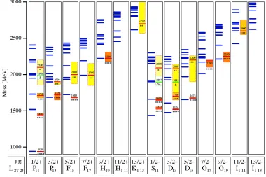
Although the list of known resonances, Table 1.1, has been updated by the PDG

group frequently, there are still many resonances missing from the SU(6)⊗O(3)

pre-dictions of the constituent quark model, especially in the mass range higher than 1.7

(19)

predicted and discovered N resonances is displayed in Fig. 1.7.

The ’missing’ resonance problem originates from the difference between the

num-ber of states predicted by the quark model and the numnum-ber observed. Resonances

may not have been observed due to a weak coupling of the missing states to the

reaction channel of the experiment or may not exist because the degrees of freedom

used in the quark model is incorrect. For example, fewer states are predicted in the

quark-diquark model as there are fewer degrees of freedom at low energies, but the

number of states predicted by this model is still more than the number observed in

ex-periments although less than the number of states predicted by the constituent quark

model. This means more studies are needed to determine the degrees of freedom in

quark models. A more completed knowledge of resonances will improve our

under-standing of the underlying symmetries and quark-quark interactions as resonances

reflect the dynamics and relevant degrees-of-freedom within hadrons.

Figure 1.7 The predicted N resonances and the spectrum discovered in

experiments. The blue lines are for the predictedN resonances and the

(20)

1.2 Single-Pion Photoproduction

There are several ways to probe the baryon excited states. To improve the

interpre-tation of the resonance spectrum confused by the missing resonances, the single-pion

photoproduction has its advantage; e.g. supporting evidence for a previously poorly

known ∆(2200)7/2− state was found in an analysis [15] that included results of a

recent measurement of the polarizedγp→π+nreaction [16]. In addition to the mass

and width values provided by the elastic pion-nucleon scattering, the single-pion

photoproduction process provides confirmations to the baryon excited states and

de-termines the amplitudes. The information about baryon resonances can be obtained

from the complex amplitudes of the single-pion photoproduction process, which can

be extracted from the observables. The measurement of double-polarization

observ-ables with a polarized target are needed in addition of the unpolarized cross section

and single-polarization observables, as they carry additional information about the

complex amplitudes which does not exist in the unpolarized cross section and

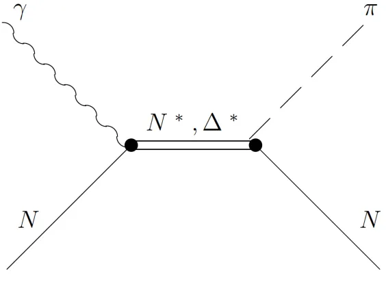
single-polarization observables. The diagram of this reaction is shown in Fig. 1.8.

Figure 1.8 The s-channel diagram of the single-pion photoproduction process with

(21)

It can be described in terms of four complex amplitudes since the product of the

number of spin states for each particle halfed by the parity conservation is four. In

the s-channel helicity representation, they are the no-flip, N, single-flip, S1 and S2,

as well as double-flip,D, amplitudes [18]. The unpolarized differential cross section,

dσ0

dΩ =|N|

2₊_|S

1|2+|S2|2+|D|2, (1.2)

cannot reveal the full information of the complex amplitudes.

Additional information, including phase relations, can be provided by polarization

observables. For example, in the helicity representation, the polarization observables

T and F are defined as

Tdσ0

dΩ = 2Im(S1N

∗₋_S

2D∗), (1.3)

and

Fdσ0

dΩ = 2Re(S2D ∗

+S1N∗). (1.4)

As polarization observables are sensitive to small amplitudes and phase differences,

they provide important constraints to reveal the dynamics and relevant

degrees-of-freedom within hadrons. In addition to the single-polarization observables (S), the

double-polarization observables are categorized into three types: beam-target (BT),

target-recoil (TR), and beam-recoil (BR) asymmetries. Since the recoil polarization

is difficult to measure for the pion-proton finalstate, the most common observables

in experiments are the single-polarization observables and the beam-target

double-polarization observables. A complete list of all pseudoscalar photoproduction

observ-ables is shown in Table 1.2.

1.3 Formalism

For the single-pion photoproduction reaction, with a polarized photon beam and a

(22)

Table 1.2 A complete list of all pseudoscalar photoproduction observables [18]

Symbol Helicity Representation Type

dσ0

dΩ |N|

2₊_|S

1|2+|S2|2+|D|2 S

Σdσ0_d_Ω 2Re(S₁∗S2 −N D∗) S

Tdσ0_d_Ω 2Im(S1N∗−S2D∗) S

Pdσ0

dΩ 2Im(S2N

∗₋_S

1D∗) S

Gdσ0_d_Ω −2Im(S1S2∗+N D

∗₎ _BT

Hdσ0_d_Ω −2Im(S1D∗−S2N∗) BT

Edσ0_d_Ω |N|2_{− |S}

1|2+|S2|2− |D|2 BT

Fdσ0_d_Ω 2Re(S2D∗+S1N∗) BT

Oxdσ0_d_Ω −2Im(S1N∗+S2D∗) BR

Ozdσ0_d_Ω −2Im(S2S1∗+N D

∗₎ _BR

Cxdσ0_d_Ω −2Re(S2N∗+S1D∗) BR

Czdσ0_d_Ω −|N|2− |S1|2+|S2|2 +|D|2 BR

Txdσ0_d_Ω 2Re(S1S2∗+N D

∗₎ _TR

Tzdσ0_d_Ω 2Re(S1N∗−S2D∗) TR

Lxdσ0_d_Ω 2Re(S2N∗−S1D∗) TR

Lzdσ0_d_Ω −|N|2+|S1|2+|S2|2− |D|2 TR

Table 1.3 Beam-target observables in single-pion photoproduction

Photon

unpolarized circularly polarized linearly polarized

Target

unpolarized dσ/dΩ - Σ

longitudinally - E G

transversely T F H,P

cross section is given as [18]

dσ dΩ =

dσ0

dΩ (1−P`Σ cos(2α)

+PX[−P`Hsin(2α) +PF]

−PY [−T +P`Pcos(2α)]

−PZ[−P`Gsin(2α) +PE]) , (1.5)

where P is the right-circular beam polarization, P` is the linear beam polarization

(23)

the target polarization in the x,y, andz directions, respectively.

For experiments with circularly polarized beam and transversally polarized target,

P` = 0 and, because the z-axis is perpendicular to the target polarization, PX =

PT cos(ϕ), PY =PT sin(ϕ), andPZ = 0, Eq. (1.5) can be simplified to

dσ dΩ =

dσ0

dΩ (1 +PTT sin(ϕ) +PTPF cos(ϕ)) , (1.6)

where PT is the target polarization and ϕ the angle from the reaction plane to the

target polarization direction. The reaction is shown in Fig. 1.9.

Figure 1.9 Schematic of the γp→π0_p _{reaction in the center-of-mass frame with}

circularly polarized photon beam and transversally polarized target.

1.4 Previous Measurements and Theoretical Predictions

The research of pion photoproduction reactions started in 1970s. By the end of 1979,

the first experimental data were taken and analyzed in several research facilities, by

M. Fukushima [19], P. Feller [20], P.J. Bussey [21], and P.S.L. Booth [22]. As the

spearhead in this area, although the precision of the data analysis was limited by

immature experimental equipment and computing technology, the research in that

(24)

proton resonance properties. Moreover, the pioneers of that era have built a solid

foundation for the following research. For example, I. S. Barker, A. Donnachie, and

J. K. Storrow [18] established the formalism for the research of pion

photoproduc-tion reacphotoproduc-tions. Another important publicaphotoproduc-tion was made by D. Besset in 1979 [23].

It explaines the procedure and the necessary estimators in the data analysis of

po-larization measurements, which solved some technical problems with the data from

real-world detectors such as the nonuniform acceptance of detectors.

In 1990s, as some reasearch facilities of the new generation became operational,

the study of pion photoproduction reactions continued developing. Besides the CLAS

detector at Jefferson Lab, the Bonn Electron Stretcher Accelerator (ELSA) and the

Mainz Microtron (MAMI) are among the most advanced reasearch facilities for

pho-toproduction reactions.

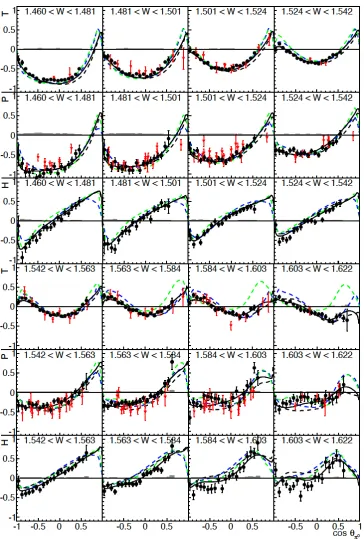
In the year of 2014, J. Hartmann et al. [24] published their experimental results

of observableT on the photoproduction of neutral pions at ELSA. Their results cover

the center-of-mass energy W range from 1.460 GeV to 1.622 GeV and are shown

in Fig. 1.10. The result from J. Hartmann et al. found no evidence for additional

structures beyond established resonances and the N(1520)3/2− helicity amplitudes

are deduced.

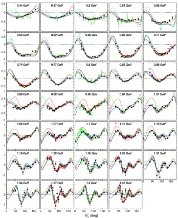
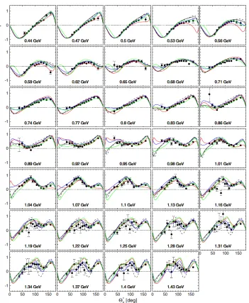
Experimental data ofT andF from MAMI were published by J. R. M. Annand et

al. [25] in 2016. The photon energies of their results are from 425 MeV to 1445 MeV

as shown in Fig. 1.11 and Fig. 1.12. The result from J. R. M. Annand et al. shows

the presence of the resonancesN(1520)3/2− _and _N_(1680)5_/₂+ _{and their interference}

with ∆(1232)3/2+_{, ∆(1700)3}_/₂−_{, and ∆(1950)7}_/₂+ _{and nonresonant background.}

So far, the results of observables T and F in this analysis agree with previous

measurements in the overlapped range of energies. The major difference between the

results in this analysis and the results from previous measurements is the difference

(25)

(26)

Figure 1.11 The T observable from J. R. M. Annand et al. [25]. The data (filled circles) are compared to experimental data (triangle) and predictions from MAID (red), SAID PR15 (blue), BG2014-2 (black), and JuBo2015-B (green).

is much larger, up to 2850 MeV, compare to the photon energy of 1445 MeV from the

most recent measurement. This will make it possible for the theoretical researchers

to study the pion photoproduction of this reaction channel in a much larger energy

range.

(27)

Figure 1.12 The F observable from J. R. M. Annand et al. [25]. The data (filled circles) are compared to experimental data (triangle) and predictions from MAID (red), SAID PR15 (blue), BG2014-2 (black), and JuBo2015-B (green).

of development in recent years, the theoretical researchers in this area are also

updat-ing their fits to newer data. There are several leadupdat-ing groups focusupdat-ing on the

devel-opment of their models through partial-wave analyses of experimental data, such as

the SAID partial-wave analysis [26], Bonn-Gatchina partial-wave analysis [27], and

(28)

Jülich-Bonn group [29]. Currently, the SAID MA27 is the latest prediction for the

polarization observables T and F. The SAID predictions were frequently updated

since the SM95 solution.

The complex amplitudes that determine the pion-photoproduction reaction

re-quire eight observables to make a complete partial-wave analysis. However, the

exist-ing data consist mainly of unpolarized cross sections and sexist-ingle-polarization

observ-ables. Thus, data of double-polarization observables, especially in the energy range

that was not included in previous measurement, become useful for the partial-wave

analysis to fulfill the completeness in the determination of the pion-photoproduction

reaction.

The purpose of this work is to extract polarization observables T and F for the

single-pion photoproduction reaction in order to be used for the partial-wave analysis

to fulfill the completeness in the determination of the pion-photoproduction reaction

and study the pion photoproduction of this reaction channel in a much larger energy

range. The data will partially solve the problem of the incomplete set of required

ob-servables that determine the pion-photoproduction for further partial-wave analyses

and the extraction of proton resonance properties. The details of the methods in this

(29)

Chapter 2 Experiment

This experiment, E03-015 “Pion Photoproduction from a Polarized Target” [30], was

conducted at the Thomas Jefferson National Accelerator Facility (Jefferson Lab) [31].

As one of 17 national laboratories funded by the U.S. Department of Energy, the

primary mission of the laboratory is to conduct basic research of the atom’s nucleus

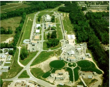
and its fundamental constituents [32]. Jefferson Lab is located in Newport News,

VA. An aerial view of the Continuous Electron Beam Accelerator Facility (CEBAF)

accelerator complex and domed, partly underground experimental Halls A, B, and C

in the foreground, is shown in Fig. 2.1.

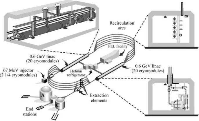
Figure 2.2 shows a schematic overview of the CEBAF accelerator and experimental

halls. Longitudinally polarized electrons from the electron source were accelerated to

67 MeV and injected into the accelerator. The electrons were accelerated up to 6 GeV

after five accelerating passes through pairs of antiparallel 600 MeV linear accelerators

(linacs) connected by recirculation arcs and delivered to the experimental halls. The

maximum capacity of this system was to deliver highly polarized continuous-wave

beams to three experimental halls with a current of up to 200 µA. The beam had a

2.004 ns bunch structure. The facility has now been upgraded to accelerate electrons

up to 12 GeV and includes a new Hall D.

The data of the experiment for this analysis were taken as part of the g9 run group

from March 18 to August 12, 2010 using the CEBAF large acceptance spectrometer

(CLAS) in Hall B at Jefferson Lab. An overview of experimental parameters of the

(30)

Figure 2.1 Areal view of Jefferson Lab with the Continuous Electron Beam Accelerator Facility (CEBAF) and experimental halls before the 12 GeV energy upgrade. This figure is from [32].

2.1 Photon Beam

After receiving the accelerated electrons from the CEBAF accelerator, a polarized

photon beam was produced by using the bremsstrahlung technique. Figure 2.3 shows

an overview of the Hall B photon tagger [34]. Longitudinally polarized electrons

were incident on the radiator and produced circularly polarized tagged photons as

the bremsstrahlung radiation of the incoming electrons. The energy of the outgoing

photonEγ was determined from the energy of the incident electronE0 and the energy

of the electron after the bremsstrahlung reaction Ee. Neglecting the small energy

transfer to the nucleus,

(31)

Figure 2.2 Overview of the CEBAF accelerator and experimental halls. The electrons were injected and accelerated up to 6 GeV then delivered to experimental halls. This figure is from [33].

The energy of the outgoing electron was determined by a magnetic spectrometer.

Electron hits in any of 384 narrow scintillators (E-counters) determined the electron

path through the tagger magnet. The scintillators in the E-plane were partially

overlapped to increase segmentation and a photon-energy resolution of 0.001E0 were

achieved. The time of the hits were also determined in a similar way by 61 T-counters

and allowed for the determination of the start time of the events of interest. The

maximum range of the tagged photon energy was 20% to 95% of the energy of the

incoming electron beam. The size of the scintillators in the E-plane had a thickness of

4 mm, a length of 20 cm, and a width that ranged from 6 to 18 mm. The scintillators

in the T-plane were 20 mm thick and the scintillators in the E-plane were 4 mm thick.

The T-plane provided a time resolution of 300 ps.

For the circularly polarized photon beam, the polarization was determined by the

polarization of the electron beam, the energy of the electron beam, and the energy

(32)

Figure 2.3 Overview of the Hall B photon tagger. Longitudinally polarized electrons were incident on the radiator and produced circularly polarized tagged photons as bremsstrahlung radiation of the incoming electrons. This figure is from [34].

2.2 FROST Target

The FROzen Spin Target (FROST) [35] was used in the g9 experiment. It was

particularly designed for the experimental study of baryon resonances with the large

acceptance CLAS detector. Particle detection over a large polar angle up to 135◦

was permitted by the FROST target. The major components of FROST include the

polarizing magnet, the dilution refrigerator, target material, and the holding coils.

The material of the FROST target is butanol and centered at z = 0 and covered

a range of 52.7 mm along the beamline. Additional 1.5-mm thick carbon and 3.5-mm

thick polyethylene disks were mounted approximately 9 cm and 16 cm downstream

of the butanol sample. The target material (butanol) was polarized with microwaves

via Dynamic Nuclear Polarization (DNP) in the field generated by the polarizing

magnet with a maximum field of 5.1 T. The target was then cooled to a temperature

less than 50 mK without the microwaves and the polarization was maintained with

(33)

shown in Fig. 2.4.

Figure 2.4 Sectional view of the frozen spin target [35]. A, beam pipe; B, LHe

inlet; C, 3He pump port; D, 4 K pot; E, 1 K pot; F, 1 K heat exchanger; G, still; H,

vacuum chamber; I, sintered heat exchanger; J, mixing chamber; K, holding coil; L, target cup; M, target insert; N, 1 K heat shield; O, 20 K heat shield; P, beam pipe

heat shield (one of three); Q,3He pump tube; R, copper cold plate; S, waveguide; T,

precool heat exchanger.

The target polarization was measured by the Nuclear Magnetic Resonance (NMR)

measurements [35]. There were two NMR systems in the g9 experiments. The first

system was utilized during the DNP process and was tuned to 212.2 MHz. The second

system was utilized when the spin was frozen and was tuned to 21.9 MHz. The result

of the NMR measurements is discussed in Chapter 3.

When operated, the system could run continuously for a typical period of 6

months. During the full length of the running period, there were several cycles

separated by the flip of the polarization direction of the target. The flips of the

polarization direction are useful in the analysis and are explained in Sec. 3.8. A

typical cycle of operation started with the dynamic nuclear polarization process with

a maximum field of 5.1 T. After the target was polarized to approximately 90%, it

was cooled by with a 3_He–4_{He dilution refrigerator to below 50 mK and the field}

of the holding coils held the polarization of the target for several weeks until the

polarization reached approximately 70% in the g9b experiment. The cycles of the

(34)

Figure 2.5 Cycles of the operation of the frozen spin target [35]. Three full operation cycles are shown. The polarization direction of the target is flipped between two adjacent cycles.

A carbon target was placed down stream to provide bound protons to measure

the bound nucleon background of the butanol data since the butanol-target events

contain both free-proton and bound-proton events. In the g9b experiment, the carbon

target was placed approximately 9 cm downstream of the butanol target.

2.3 CLAS Detector

The CEBAF Large Acceptance Spectrometer (CLAS) [36] was based on a multigap

magnet with six super-conducting coils, symmetrically arranged to generate an

ap-proximately toroidal field distribution. The CLAS detector has been used for various

experiments including the present pion photoproduction experiment. One distinct

aspect of the CLAS detector was the large-acceptance detection with a polar-angle

range from 8◦ to 142◦. It is particularly suited in the study of reactions with low

lu-minosity (e.g., experiments using a tagged-bremsstrahlung photon beam) or reactions

with multi-particle final states. The CLAS detector had several major parts including

the torus magnet, the time-of-flight counters, the Cherenkov counters, and the drift

chambers. The schematic view of the CLAS detector can be found in Fig. 2.6. This

design made it possible to detect final-states particles in a wide angular range.

An-other schematic view of the CLAS detector cut perpendicular to the beam is shown

(35)

Figure 2.6 Schematic view of the CLAS detector, including drift chambers, Cherenkov counters, electromagnetic calorimeter, and the time-of-flight counters. These detectors cover almost the entire sphere except the very forward and backward angles along the beamline. This figure is from [37].

The purpose of the torus magnet [38] in the CLAS detector was to analyze the

momentum of the final-states particles with the tracking assistance of the drift

cham-bers. The magnetic field was generated by six coils installed around the beam line.

Each coil consisted of four layers of 54 turns of aluminum-stabilized NbTi/Cu

super-conductor and was cooled to 4.5 K by liquid helium through cooling tubes located

at the edge of the windings. The maximum current was 3860 A with a maximum

integral magnetic field of 2.5 Tm.

The contours of constant magnetic field in the midplane between two coils are

(36)

Figure 2.7 Schematic view of the CLAS detector perpendicular to beam [36]. These detectors have a large azimuthal coverage.

was set to positive, the positively charged particles were bent toward the beam axis

and the negatively charged particles were bent away from the beam axis. When the

current was set to negative, the positively charged particles were bent away from

the beam axis and the negatively charged particles were bent toward the beam axis.

In the g9 experiment, the system was running at +1920 A to moderately bend the

positively charged particles and negatively charged particles toward and away from

the beam axis, respectively, and make both positively and negatively charged particles

have large acceptances over the θlab _angle.

The drift chambers [39] were used to track the final-state charged particles. In the

(37)

Figure 2.8 The magnetic field for the CLAS toroid in the midplane between two coils [36].

charged particle traveled through a drift chamber, the drift cells along its trajectory

were triggered. By aligning the triggered drift cells, the trajectory of the particle

was known. The three momentum and the charge of the particles were calculated

from the trajectory of the particle and the magnetic field. The track length and the

reaction vertex were also reconstructed by using information of particles from the

drift chambers. This process is illustrated in Fig. 2.10 [39].

The CLAS time-of-flight system [40] consisted of 57 scintillator paddles in each

of the six sectors. Each scintillator paddle was 5.08 cm thick and 15 or 22 cm wide,

with lengths from 32 cm at the most forward angle to 450 cm at larger angles. For

each scintillator paddle, two photomultiplier tubes were placed at both ends of the

scintillator paddle. The whole area of coverage was 206 m2_{. The view of TOF counters}

in one sector is shown in Fig. 2.11 [40]. The performance of the system allowed for

particle separation by using the time-of-flight information measured for momenta up

to 2 GeV due to a time resolution of typically 150 ns.

(38)

Figure 2.9 The magnetic field orientation. Magnetic field vectors transverse to the beam in a plane centered on the target [36].

placed right outside the target. It was used to measure the start time of events. A

sketch of the start counter is shown in Fig. 2.12. Outgoing particles produced light

in the 2.2-mm thick scintillators and triggered signals in the PMTs that were coupled

to the scintillators with a light guide. The time resolution of the start counter was

350 ps. It is less than the 2.004 ns bunch structure of the beam.

2.4 Beamline Devices

To measure the electron beam position, three beam-position monitors were installed

(39)

Figure 2.10 The drift process measured by the drift chambers [39]. The drift cells of region 3 along its trajectory that triggered are drawn in dark.

(40)

Figure 2.12 Sketch of the start counter [41].

position and intensity were measured with a measurement rate of about 1 Hz. The

profile of the electron beam was also measured. Thin wires were moved through the

beam and scattered electrons were detected to reconstruct the electron beam profile.

The wires were oriented along the horizontal and vertical axes with the moving device

(harp). There were three harps installed at 36.7, 22.1, and 15.5 m upstream of the

target.

The Møller measurements [36] was used to measure the electron-beam

polariza-tion. It was installed upstream of the tagging system. To make a high-precision

measurement of the beam polarization, the asymmetry in elastic electron-electron

scattering has been measured. The scattering target was a 25-µm thick permendur

foil, magnetized with a Helmholtz-coil system. Additionally, there are two quadrupole

magnets and two detectors on both sides. The scattered electrons were detected in

coincidence to determine the reaction kinematics. The Møller measurements were

(41)

Chapter 3 Data Analysis

For theγp→π0_p_{reaction in the FROST g9b experiment with CLAS, the circularly}

polarized tagged photons in the energy range from 0.62 GeV to 2.93 GeV of the

electron beam were produced by the radiator of the Hall-B Photon Tagger from

incident longitudinally-polarized electrons with energies of 3.082 GeV. The

photon-beam helicity was flipped pseudo randomly at a rate of 240 Hz or 30 Hz. The

collimated photon beam irradiated the FROST target. The nuclear spin of free

protons in the target was polarized and the target polarization direction was changed

periodically. A carbon target and a polyethylene target were used downstream of

the butanol target for background subtraction and comparison use. The final-state

protons from those targets were detected by the CLAS detector.

3.1 Beam and Target Polarizations

The circularly polarized tagged photons were produced by the Bremsstrahlung process

from incident longitudinally polarized electrons. The polarization of the photon beam

depends on the ratio between the photon energy Eγ and the electron energy E0.

Specifically, the degree of the circular polarization is expressed as [42]

P =Pe

4x−x2

4−4x+ 3x2, (3.1)

where x=Eγ/E0.

The electron-beam polarization was measured by Møller measurements [43]. The

(42)

and was found to be consistent with a constant polarization throughout the

ex-periment. The average electron-beam polarization and statistical uncertainty are

Pe = 0.873±0.006, while the systematic uncertainty of Møller measurements in Hall

B were 3% [43]. The electron-beam helicity was pseudo-randomly flipping at a rate

of 240 Hz (30 Hz for the Møller measurements). The g9b experiment ran

concur-rently with the Qweak experiment [44]. The helicity reporting was delayed. This

is common for parity-violation experiments, like Qweak, with special demanding

re-quirements on helicity-correlated beam properties. The beam helicity of a given event

was determined during initial data analysis and stored event-by-event in the event’s

header bank (HEAD): bit 29 contains the helicity bit of the event and bit 30 indicates

whether or not the helicity was correctly reconstructed [43].

Figure 3.1 The electron-beam polarization measured by the Møller measurements.

The horizontal line indicates the mean value of the six measurements.

The free protons in the butanol target were transversally polarized by dynamic

nuclear polarization and kept at low temperature [35]. The target-polarization

direc-tion was oriented at an angle ϕ0 with respect to the horizontal direction in the lab

frame (xlab_{) for the nominally positive polarization direction. The angle} _ϕ _between

(43)

event from the measured azimuthal angle of the detected proton,ϕlab

p ,

ϕ=−ϕlab

π +ϕ0 =π−ϕlabp +ϕ0. (3.2)

All relevant angles are illustrated in Fig. 3.2. In this analysis a value ofϕ0 = 116.3◦±

1.4◦ was used that was determined in a moment-method analysis, see Sec. 3.8.

ylab

p_π

p_p

xlab

ϕ_π ϕ₀

ϕ_p

Reaction plane

Target-polarization orientation

ϕ

x

lab

Figure 3.2 Target polarization orientation in the lab- and reaction frames.

The Nuclear Magnetic Resonance (NMR) measurements provide the degree of

tar-get polarization. The tartar-get polarization values were determined by Y. Mao in [45].

The target polarization as a function of the run number is shown in Fig. 3.3. Spin

alignments along theϕ0 = 116.3◦ direction are marked with blue symbols; alignments

in the opposite direction are marked with red symbols. The target polarization

de-creased with time and the target was routinely repolarized to the opposite direction

after a number of runs. The relaxation time during g9b was about 3400 h for positive

polarization with beam and 4000 h without [35]. In this analysis it was assumed that

the magnitude of the target polarization is constant within a given run.

An experimental asymmetry signal from the butanol target was analyzed for each

(44)

Figure 3.3 The target polarization of the run groups used measured by NMR. Spin

alignments along the nominally positive direction (ϕ0 = 116.3◦) are marked with

blue symbols; alignments in the opposite direction are marked with red symbols. The change of color indicates the target was repolarized to the opposite direction.

investigate systematic uncertainties in the target polarization. The raw asymmetry

of observableF served for that purpose, Eq. (3.27) withh= 1, as detector acceptances

cancel for this observable but not for observable T. The raw asymmetry is inversely

proportional to the product of electron beam and target polarizationsPePT, Eq. (3.1)

and Eq. (3.27). For the center-of-mass energy range from W = 1.5 GeV to 1.9 GeV

and the cosθ range from−0.4 to 0.8, the average raw asymmetry is shown in Fig. 3.4

as a function of run number for the runs used in this analysis. The figure also shows

the mean values for each of the five run groups (red horizontal lines) and the mean

value over all runs (black horizontal line).

Table 3.1 gives the values for those mean values with their statistical uncertainties.

The result indicates that the raw asymmetries of all run groups are consistent with

each other within their relative uncertainties of 3% to 4%. Within that range, there is

no indication of run-group-dependent systematic uncertainties of the product PePT.

(45)

Figure 3.4 The raw asymmetry, Eq. (3.27) with h= 1, of the butanol-target events for the run groups 1 through 5 used in the analysis. The horizontal red lines

indicate the mean values for the five run groups and the black line indicates the average raw asymmetry over all runs.

Table 3.1 Raw asymmetry of the butanol-target events for the first 5 run groups.

Run group Raw Asymmetry (F)

1 0.0526±0.0021

2 0.0494±0.0018

3 0.0485±0.0019

4 0.0489±0.0015

5 0.0491±0.0016

Avg. 0.0495±0.0008

and the 4% difference of measured FROST target polarizations with two separate

NMR coils reported in [35].

The run information for all run groups is summarized and listed in Table 3.2. The

group number, the run-number range, incident electron-beam energy, the number of

events, the frequency of the helicity flip, the target polarization, and the orientation of

the target holding field [46] are given. The target magnet quenched from a power surge

(46)

10 contain only 22% of the statistics and were run with an average target polarization

that was about a factor of 0.75 smaller. Assuming everything else being equal, that

would result in statistical uncertainties of results from run groups 6 through 10 that

are about a factor 3 larger than for results of the first five run groups. On the

one hand, including the final five run groups in a combined result could improve

the statistical uncertainty by merely 6%. On the other hand, additional systematic

uncertainties could affect the final result, given that the replacement target had a

different geometry than the original one. In this analysis only the first five run

groups were used.

Table 3.2 The g9b run information for circularly polarized beam runs. Given are

the group number, the run number, incident electron-beam energy, the number of

primary events, the frequency of the helicity flip f, the target polarization and the

sign of the target polarization, and the orientation of the target holding field [46].

Group Run range Ee (GeV) Events f (Hz) Target pol. Field

1 62207 - 62289 3.082 723.1 M 240 .83 - .80 (+) (+)

2 62298 - 62372 3.082 894.9 M 240 .86 - .80 (−) (+)

3 62374 - 62464 3.082 1129.7 M 240 or 30 .79 - .75 (+) (+)

4 62504 - 62604 3.082 1307.1 M 240 .81 - .76 (−) (−)

5 62609 - 62704 3.082 972.6 M 240 or 30 .85 - .79 (+) (−)

runs not used in this analysis

6 63508 - 63525 2.266 138.2 M 943 .77 - .58 (+) (+)

7 63529 - 63542 2.266 166.8 M 240 or 943 .56 - .57 (−) (−)

8 63543 - 63564 2.266 321.7 M 943 .74 - .61 (+) (+)

9 63566 - 63581 2.266 249.6 M 943 .70 - .64 (−) (−)

10 63582 - 63598 2.266 242.3 M 240 .48 - .46 (+) (+)

3.2 Reaction Vertex

The reconstructed reaction vertex were utilized to categorize events from the butanol,

carbon, and polyethylene targets in the beamline. Two distributions of thez

coordi-nate of the reconstructed reaction vertex are shown in Fig. 3.5 for different W and

(47)

coordinate of the reconstructed reaction vertex. The z-range of the butanol target

was chosen to align with the highest average raw asymmetry from z = −3 cm to

z = 2 cm. The raw asymmetry of observable F starts to decrease beyondz = 2.0 cm

as shown in Fig. 3.6 because the fraction of events from polarized protons starts to

decrease as the reconstructed reaction vertex is approaching the end of actual target

at z = 2.5 cm. This cut helps to maintain a high average dilution factor. A wider

cut would have increased the overall statistics of the data but at the expense of a

more diluted asymmetry signal. The ranges of the appliedz-vertex cuts for the three

targets are listed in Table 3.3.

Table 3.3 Selection criteria for the three targets based on the reconstructed z

coordinate of the reaction vertex.

Target Reaction Vertex (z)

Butanol −3 cm to 2 cm

Carbon 8 cm to 11 cm

Polyethylene 14 cm to 17 cm

Following Ref. [48] additional cuts have been applied on the transverse vertex

coordinates to suppress the fraction of poorly reconstructed proton tracks. The x

coordinate andycoordinate of the reconstructed reaction vertex are shown in Fig. 3.7.

The distribution peaks at (x, y) = (−0.31 cm,−0.28 cm) and only events with a

transverse distance of less than 2 cm from that point were kept in the analysis.

3.3 Particle Identification and Coincidence Time

To identify final-state protons in coincidence with the initial-state photons, events

with one positively charged particle and zero negatively charged particles were

con-sidered.

The time-of-flight difference of the positively charged particle in each event ∆tp

(48)

Figure 3.5 Examples of the reconstructed z-vertex distributions of protons. The

main structures in the distribution are from the butanol (z ≈0), carbon (z ≈9 cm),

and polyethylene (z ≈16 cm) targets. According to the implementation of the

target geometry in Ref. [47], the structure atz ≈12.5 cm comes from the 1 K end

(49)

Figure 3.6 The raw asymmetry of observable F as a function of the reconstructed

z vertex. Events within the z-range from z =−3 cm to 2 cm were chosen for the

analysis as indicated between the red lines. The raw asymmetry is increasingly diluted for z >2 cm.

calculated from the momentum p and speed β of the particle under the assumption

that the particle was a proton with rest mass mp:

∆tp =texp−tcalc=

`SC

c





1

β −

v u u t

m2

pc2

p2 + 1 

, (3.3)

where `SC is the path length from the reaction vertex to the TOF paddles and β is

determined from the time of flight and `SC. ∆tp is used to distinguish a proton from

other positively charged particles; for protons ∆tp ≈0.

The performance of all TOF paddles has been examined by checking ∆tp of each

paddle for each run group to reduce the probability of particle misidentification.

Examples are shown in Fig. 3.8. Problematic paddles were removed from the analysis

as listed in Table 3.4.

The distribution of ∆tp for positively charged particles as function of

momen-tum is shown in the left panel of Fig. 3.9. The central maximum with ∆tp ≈ 0

(50)

Figure 3.7 The reconstructed (x, y)-vertex distribution of protons. The maximum

of the distribution is at (−0.31 cm,−0.28 cm). Events within the black circle have

been selected for further analysis.

Figure 3.8 The ∆tp distributions of each paddle in sector 3 for run group 2. Paddle

(51)

Table 3.4 Paddles that were removed from the analysis for the full run range from run 62207 to 62704.

Sector Paddles

1 24, 40, 42, 43, 44

2 29, 36, 37, 39

3 23, 26, 37

4 33, 39, 40

5 23

6 —

corresponds to pions. Although most problematic TOF paddles have been removed,

timing-related issues remain visible in the distribution as narrow, almost vertical

bands at low momenta; most pronounced at about 0.5 GeV/c. These events have

signals from paddle readouts that are far smaller than the typical energy deposition

Edep in TOF paddles. The right panel of Fig. 3.9 shows the Edep distribution as a

function of particle momentum together with a momentum-dependent cut that helps

discriminating proton-candidate events with high energy deposition in the paddles

from mostly background events with a low signal in the detectors.

To select from all recorded photons the photon that led to the reaction, we also

need the CLAS-tagger coincidence time, ∆tc, which is defined as

∆tc =tv,γ−tv,p=

tγ+

z c

− tp,ST −

`ST

βc

!

, (3.4)

wheretγ is the time measured by the tagger and reported at the center of the CLAS

detector, z is the reaction vertex z coordinate, tp,ST is the proton time of the Start

Counter (ST) subsystem, and`ST is the path length of the proton from the reaction

vertex to the ST subsystem hit position. The distribution of ∆tcis shown as function

of momentum in the left panel of Fig. 3.10. The central maximum at ∆tc≈0 includes

true coincidences between the tagged photon and the event in the CLAS detector.

Side peaks are random coincidences. As previously in Fig. 3.9, the distribution of

(52)

Figure 3.9 ∆tp distribution for positively charged particles in CLAS after removing the TOF paddels of Table 3.4 (left panel). Remaining timing issues are visible in the almost vertical stripes at low momenta. The right panel shows the

measured energy deposition Edep in the TOF paddles as a function of particle

momentum along with a momentum-dependent cut on that helps suppressing background events with small signals in the detectors.

Figure 3.10 The left panel shows the CLAS-tagger coincidence time ∆tc with a

shift at low momentum due to large energy loss of low-energy protons. The

selection of coincident events is shown in red. The right panel shows the ∆tp

distribution for positively charged particles in CLAS after applying the momentum

dependent cut onEdep. Events between the red curves were selected as protons in

(53)

the momentum-dependent Edep cut that effectively suppresses the background from

misidentified particles. The ∆tc and ∆tp distributions are slightly asymmetric at low

momenta due to the large energy loss of low-momentum protons. Event selections

were made in either case with complex momentum-dependent cuts. The ∆tcand ∆tp

distributions were sliced in 0.2-GeV/c wide momentum bins and fitted with gaussian

distributions. The cut limits in the center of each momentum bin were chosen as

±2σ off the distribution’s maximum. An example of a gaussian fit to ∆tc data for

one slice in momentum between 1.4 GeV/c and 1.6 GeV/c is shown in Figure 3.11.

Figure 3.11 An example of the fitting in one momentum slice for the complex ∆tc

selection cut. It shows the gaussian fit of the ∆tc distribution in the momentum

range from 1.4 GeV/c to 1.6 GeV/c.

Figure 3.12 shows the integrated ∆tc and ∆tp distributions for various selection

criteria: for the raw data, after applying the momentum dependent ∆tp and ∆tccuts,

(54)

Figure 3.12 The left panel shows the CLAS-tagger coincidence time distribution for various selection criteria. The right panel shows the time distribution of proton candidates for various selection criteria.

reaction close to M_π20. After the reaction-channel selection with a missing mass cut,

the background from random coincidences appears to be less than 2% based on the

yields in the true and random coincidence peaks. Proton misidentification appears

to be negligible.

3.4 Corrections

The standard eloss package [47] was utilized to determine from the measured

momen-tum the momenmomen-tum of the protons at the reaction vertex in the target. The correction

accounts for energy losses in the target material, target wall, carbon cylinder, and

start counter. Additionally, momentum corrections were applied to the detected

pro-tons following the procedure of CLAS Note 2013-011, “Momentum corrections forπ+

and protons in g9b data” [49]. These momentum corrections make an attempt to

correct errors in the momentum determination that may be caused by drift-chamber

(55)

) 4 /c 2 (GeV X 2 M 0.4

− −0.2 0.0 0.2 0.4

Events

0 1000 2000 3000

Missing Mass Squared W = 1.565 GeV

) = -0.45

π θ

cos( 0.01

±

h = 0.57

Missing Mass Squared

) 4 /c 2 (GeV X 2 M 0.4

− −0.2 0.0 0.2 0.4

Events

0 500 1000

Missing Mass Squared W = 1.715 GeV

) = 0.25

π θ

cos( 0.01

±

h = 0.48

Missing Mass Squared

) 4 /c 2 (GeV X 2 M 0.4

− −0.2 0.0 0.2 0.4

Events

0 100 200 300

W = 1.895 GeV ) = -0.15

π θ

cos( 0.02

±

h = 0.57

) 4 /c 2 (GeV X 2 M 0.4

− −0.2 0.0 0.2 0.4

Events 0 20 40 60 80

W = 2.225 GeV ) = 0.55

π θ

cos( 0.03

±

h = 0.35

Figure 3.13 Examples of missing-mass-squared distributions from butanol-target

(black histograms) and carbon-target data (gray histograms). The solid red and green curves are fits to the butanol and carbon data, respectively. The scaled carbon-data fit is shown as red dashed curve and the scaled carbon distribution as

green histogram. Also indicated are the dilution factorsh.

3.5 Channel Identification

The channel identification process was based on individual kinematic bins. The data

were binned in W from 1.49 GeV to 2.51 GeV with a bin size of 0.03 GeV and in

cosine of the center-of-mass angle, cosθcm

π , from −1 to 1 with a bin size of 0.1. The

missing-mass-squared distributions in the γp→pX reaction from both butanol and

carbon targets were accumulated for each bin. Figure 3.13 shows four examples of

missing-mass distributions for various energy and angular bins.

The black histograms show data from the butanol target and the gray histograms,

with much smaller statistics, show data from the carbon target. The central peaks

(56)

at M2

X = m2π0 ≈ 0.018 GeV2/c4 above a broad background correspond to events

from the γp → π0_p _{reaction off free protons in the butanol target. To determine}

the bound-nucleon background in the missing-mass-squared distributions from the

butanol target, a composite fit was applied to each distribution. For each bin, the

carbon-target distribution was described with a cubic splinep3(x) with four nodes and

the butanol-target distribution was described by the same spline function multiplied

by a scale factor for the bound-nucleon background and a gaussian function for the

free-proton events of the expected reaction channel. The fit functions that described

the signal,S(x), the carbon-target,C(x), and the butanol-target,B(x), distributions

are

S(x) = Y0exp −

(x−M₀2)2 2σ2

!

, (3.5)

C(x) = p3(x;x1, y1, x2, y2, x3, y3, x4, y4, b2, e2), and (3.6)

B(x) = κC(x) +S(x). (3.7)

The signal parameters Y0,M02, andσ, the parameters of the spline functionxi,yi,

and the second derivative at the first and last nodes, b2 and e2, respectively, as well

as the scale factorκ were determined by simultaneous fits to the carbon and butanol

distributions. The quantity

χ2_MLE = 2

X

i

[B(M_i2)−N_iB·logB(M_i2)] +X j

[C(M_i2)−N_jC ·logC(M_j2)]

(3.8)

was minimized in the fits. It is the sum of the negative logarithm of the likelihood

function for Poisson-distributed butanol and carbon data. Those functions introduce

the least bias in the estimation of the parameters [50]. The first sum in Eq. (3.8) runs

over all bins in the butanol missing-mass-squared distribution within a specified fit

range, listed in Table 3.5, and the second sum runs similarly over bins in the

carbon-data histograms. NB

k and NkC are the number of events in the bins of the butanol

and carbon histogram at a missing-mass-squaredM2

k. The minimization of Eq. (3.8)

How to Make a Mudsparkler

University of South Carolina

Scholar Commons

Polarization Observables T and F in the yp -> pi p

Reaction

Hao Jiang

Acknowledgments

Abstract

Table of Contents

List of Tables

List of Figures

Chapter 1

Introduction

Chapter 2

Experiment

Chapter 3

Data Analysis