https://doi.org/10.5194/nhess-18-303-2018 © Author(s) 2018. This work is distributed under the Creative Commons Attribution 4.0 License.
Comparing thixotropic and Herschel–Bulkley parameterizations for
continuum models of avalanches and subaqueous debris flows
Chan-Hoo Jeon1,2and Ben R. Hodges2
1Division of Marine Science, The University of Southern Mississippi, 1020 Balch Blvd, Stennis Space Center, Mississippi 39529, USA
2Center for Water and the Environment, The University of Texas at Austin, Austin, Texas 78712, USA Correspondence:Chan-Hoo Jeon ([email protected])
Received: 10 July 2017 – Discussion started: 17 July 2017
Revised: 1 December 2017 – Accepted: 4 December 2017 – Published: 22 January 2018
Abstract. Avalanches and subaqueous debris flows are two cases of a wide range of natural hazards that have been pre-viously modeled with non-Newtonian fluid mechanics ap-proximating the interplay of forces associated with grav-ity flows of granular and solid–liquid mixtures. The com-plex behaviors of such flows at unsteady flow initiation (i.e., destruction of structural jamming) and flow stalling (restructuralization) imply that the representative viscosity– stress relationships should include hysteresis: there is no rea-son to expect the timescale of microstructure destruction is the same as the timescale of restructuralization. The non-Newtonian Herschel–Bulkley relationship that has been pre-viously used in such models implies complete reversibility of the stress–strain relationship and thus cannot correctly represent unsteady phases. In contrast, a thixotropic non-Newtonian model allows representation of initial structural jamming and aging effects that provide hysteresis in the stress–strain relationship. In this study, a thixotropic model and a Herschel–Bulkley model are compared to each other and to prior laboratory experiments that are representative of an avalanche and a subaqueous debris flow. A numer-ical solver using a multi-material level-set method is ap-plied to track multiple interfaces simultaneously in the sim-ulations. The numerical results are validated with analyti-cal solutions and available experimental data using param-eters selected based on the experimental setup and without post hoc calibration. The thixotropic (time-dependent) fluid model shows reasonable agreement with all the experimental data. For most of the experimental conditions, the Herschel– Bulkley (time-independent) model results were similar to the thixotropic model, a critical exception being conditions with
a high yield stress where the Herschel–Bulkley model did not initiate flow. These results indicate that the thixotropic rela-tionship is promising for modeling unsteady phases of debris flows and avalanches, but there is a need for better under-standing of the correct material parameters and parameters for the initial structural jamming and characteristic time of aging, which requires more detailed experimental data than presently available.
1 Introduction
pro-vide further challenges as we simply do not have an ade-quate and proven theory for representing their behavior at natural-hazard scales. Indeed, even if we develop a complete and practical theory for the movement of a mixture of fluid, particles, and entrained large objects across several magni-tudes of scales, it is unclear how we would effectively cap-ture the uncertainty associated with size and space distribu-tion of solid objects (e.g., boulders in a landslide) that affect the flow propagation in any model attempting to directly rep-resent fluid-solid structural interactions.
Large-scale natural-hazard flows have been widely inves-tigated with field observations, small-scale laboratory exper-iments, and numerical models. A common observation is that the complexity of the material composition and the effec-tive rheological characteristics play important roles in ma-terial movement (Malet et al., 2003; Bisantino et al., 2010; Jeong, 2014; de Haas et al., 2015). This flow complexity is illustrated by the classification of subaqueous mass move-ments by Locat and Lee (2002) into five types with differ-ent behaviors: slides, topples, spreads, falls, and flows. At the “flow” end of the spectrum the water content is high, the particle sizes are small, and the flowing conditions are rea-sonably considered a fluid continuum. As the water content decreases and/or the particle size distribution covers more orders of magnitude, the theoretical basis for the fluid con-tinuum approach becomes weaker and requires more em-pirical parameterization to capture other behaviors. Further-more, the transition from a non-moving to a flowing regime can involve spatial heterogeneity and time-dependent behav-ior that is not well-represented by parameterizations of the flowing regime. Real-world debris flows include additional complexity as they erode and entrain material along the bot-tom and sides of the slope with the downstream flow. We take these issues as motivational for the present work and re-fer the reader to the recent review of Delannay et al. (2017) for further insight on granular flows and Shanmugam (2015) for heterogenous flows. The fundamentals physics of such flows is presented in Iverson (1997). Herein, we do not seek to distinguish between the differing physics of these vari-ous complex flows but rather focus on advancing the use of non-Newtonian viscosity models as a proxy for their general behavior. For simplicity in exposition, we will use the term “debris flow” to refer to any real-world mixture modeled as a continuum fluid using a non-Newtonian model.
Following Ancey (2007), the existing approaches to simu-lating debris flows can be categorized in three groups: (i) ap-plying soil mechanics concept of coulomb behavior, which provides reasonable solutions for heterogeneous granular mass flows (Iverson and Denlinger, 2001; Iverson, 2003); (ii) merging soil and fluid mechanics models; and (iii) rep-resenting the heterogeneous debris as a continuum fluid with behaviors similar to a non-Newtonian fluid (the approach herein) where the transition from a stable structure to a mov-ing fluid is handled as a viscous effect. This is not to imply that such flows are actually non-Newtonian fluids but merely
that some of their behaviors can be captured with an appro-priately parameterized viscosity model (e.g., Davies, 1986; Pierson and Costa, 1987; Coussot and Meunier, 1996; Pu-dasaini, 2012). Indeed, Iverson (2003) has referred to the rheological approach to debris flows as a “myth” and ar-gued for its replacement with mixture models using separate solid–fluid components. However, their argument remains contentious, and it is not clear that the present state of mix-ture models is substantially less mythical than application of a rheological model when considering heterogenous mix-tures over a wide range of scales. Given that debris flow cov-ers such divcov-erse phenomena and complex physics, it seems likely the “correct” model for the foreseeable future will be the model that best fits a specific event, experiment, or flow type of interest. In the absence of research that definitively solves the conundrum of debris flow, we follow the long his-tory of using rheological models as a proxy. Such models are parsimonious in the number of coefficients and are ef-fectively agnostic to the inherent uncertainties of fluid-solid distributions and interactions. In using a non-Newtonian rhe-ological model, the real-world interaction between solid par-ticles and surrounding fluid in a heterogeneous mixture can be thought of as similar to the microstructural behavior of a homogeneous non-Newtonian fluid where the local fluid vis-cosity is a function of the local stress. The main advantage of this approach is that a non-Newtonian rheological model is simply a time/space-dependent viscosity term for the Navier– Stokes equations. It follows that the time/space-varying eddy viscosities in a wide range of existing hydrodynamic codes can be readily adapted to non-Newtonian behavior and used for parameterized modeling of debris flows.
Note that the terminology of non-Newtonian flows can be confusing as “time-independent” models have viscosi-ties that can change with both space and time throughout a flow. The difference between a “time-independent” and a “time-dependent” non-Newtonian fluid is whether the rela-tion between stress and viscosity (i.e., non-Newtonian equa-tion itself) is allowed to change with time. Thixotropic (time-dependent) fluids are defined as non-Newtonian fluids where the process of “aging” during a flow changes the underlying fluid microstructure and the relationship between stress and viscosity (Moller et al., 2009). Herein, we examine how the use of a thixotropic model provides the ability to model be-haviors that cannot be represented with a time-independent non-Newtonian model. Our goal is to provide insight into the research needs for further experiments and model develop-ment into the natural hazards of gravity-driven debris flows across the transitions from inception to stalling.
simulate debris flows (e.g., Bovet et al., 2010; Pirulli, 2010; Tsai et al., 2011; Manga and Bonini, 2012); however the real-world flow characteristics include time-dependent behaviors that could be categorized as “thixotropic” (Perret et al., 1996; Crosta and Dal Negro, 2003; Bagdassarov and Pinkerton, 2004; Aziz et al., 2010). Our focus in this paper is examining how a thixotropic model behavior compares to the more com-mon time-independent (Herschel–Bulkley) non-Newtonian fluid model.
From a macroscale perspective, debris flows have similar behaviors to “yield-stress fluids” that have been studied as a class of non-Newtonian fluids (Møller et al., 2006; Scotto di Santolo et al., 2010). A yield-stress fluid is effectively a solid (i.e., infinite viscosity) below a critical stress value (yield stress). This behavior is similar to what might be ex-pected from a debris mixture of liquid and solids that is ini-tially at rest and is triggered into motion as the yield stress is exceeded, which is the basis for prior time-independent non-Newtonian models cited above. At the microscale under low-stress (near-rest) conditions the fluid flow around the solids in a debris mixture is inhibited by viscous boundary layers and inertia of the solids, which provides effects similar to a higher-viscosity fluid at the macroscale (i.e., low deforma-tion under stress). Once the solids in the debris have acceler-ated, the effects of particle lift, drag, and rotation induced by the surrounding turbulent fluid flow, as well as solid–solid impacts and particle disintegration, will provide behaviors similar to a lower-viscosity fluid that deforms more easily under stress. This change from high viscosity to low vis-cosity under stress is readily simulated with a conventional time-independent non-Newtonian Herschel–Bulkley model. Arguably, what is missing from a time-independent model is that the destruction of the initial microstructure of the debris can change the effective macroscale viscosity and response to stress. If the flow stalls either globally or locally, it may take some time to reestablish its microstructure, so the yield stress for a recently stalled flow should be different than the yield stress after aging (consolidation). We can think of the behav-ior of a debris flow as controlled, at least partly, by the evo-lution of the microstructure and requiring a time-dependent element in the non-Newtonian model.
The simplest non-Newtonian yield-stress fluids are Bing-ham plastics. More complex behaviors are associated with “shear thinning” and “shear thickening” where the effec-tive viscosity nonlinearly changes with the rate of strain. For these standard cases, the relationship between viscos-ity and rate of strain is repeatable and time-independent. The approach proposed by Herschel and Bulkley (1926) is a common approach for representing the general case of time-independent non-Newtonian fluids wherein the plastic vis-cosity,η, is conditional on the yield stress,τ0, as
(
η=Kγ˙n−1+τ0
˙
γ if τ > τ0
˙
γ=0 if τ ≤τ0
, (1)
whereK is the consistency parameter, n is the Herschel– Bulkley fluid index, and γ˙ is the scalar value of the rate of strain. The Herschel–Bulkley fluid indexn controls the overall modeled behavior, where 0< n <1 is shear thinning,
n >1 is shear thickening, andn=1 corresponds to the Bing-ham plastic model (BingBing-ham, 1916).
A recognized problem with numerical simulation using a Herschel–Bulkley model is the viscosity is effectively infi-nite below the yield stress; i.e., the conditionγ˙ =0 in Eq. (1) is identical toη= ∞for modeling a fluid continuum that be-comes solid below the yield stress. An infinite (or even very large) viscosity creates an ill-conditioned matrix in a discrete solution of the partial differential equations for fluid flow. Furthermore, the instantaneous transition from infinite to fi-nite viscosity as the yield stress is crossed provides a sharp change that can lead to unstable numerical oscillations. Dent and Lang (1983) attempted to resolve this issue with a bi-viscous Bingham fluid model for computing motion of snow avalanches. Their approach was shown to be reasonable us-ing comparisons with experimental data but was later deter-mined to be invalid for conditions where the shear stresses are much lower than the yield stress (Beverly and Tanner, 1992). A more successful approach was that of Papanasta-siou (1987), who proposed modifying the Herschel–Bulkley model with an exponential parameter,m. The Papanastasiou model (presented in detail in Sect. 3, below), with appropri-ate values form, shows good approximations at low shear rates for Bingham plastics (Beverly and Tanner, 1992).
Although a flow simulated with the Papanastasiou model will have changes in the viscosity with time (as the shear changes with time), the model is still deemed “time-independent” as the relationship between viscosity and shear is fixed by the selection ofK,n,m, andτ0. Arguably, there exist a wide range of debris flows over which the Papanas-tasiou approach should be adequate, as thetime-dependent
the time-independent Papanastasiou model to simulate snow avalanches with some success, but again their results showed more significant discrepancies with experiments during flow initiation. De Blasio et al. (2004) simulated both subaerial and subaqueous debris flows with a Bingham fluid model. Their results for the subaerial debris flows were in a reason-able agreement with laboratory data, but their subaqueous simulations showed a significant discrepancy with measure-ments. A clear challenge in validating models of debris flows beyond steady conditions is that the most commonly avail-able experimental data are focused on the steady or quasi-steady conditions after the debris structure has (relatively) homogenized.
Thixotropic (time-dependent) behavior, which is not rep-resented in the Herschel–Bulkley model, provides an inter-esting avenue for representing the expected macroscale be-havior of a debris flow near initiation. At rest, debris solids provide structural resistance to flow (for denser solids) and a greater inertial resistance to motion than the fluid. Thus, it is reasonable to expect initial behavior similar to a Bingham plastic, i.e., initially infinite viscosity with a high yield stress. However, the onset of motion for the debris flow begins the destruction of the microstructure, homogenization of the de-bris, and a change in the relationship between stress and vis-cosity, which might be thought of as shear-thinning behav-ior. A key difference between a Herschel–Bulkley model and the real world is that the former requires a return to struc-ture whenever the internal stress drops below the yield stress; however, in a debris flow we expect the destruction of mi-crostructure to significantly reduce the stress at which re-newal of structure (consolidation) occurs. For a real debris flow we expect different viscosity–stress behaviors during initiation, steady-state, and slowing phases (consistent with evolving microstructure), but a time-independent Herschel– Bulkley model is effectively an assumption that the pro-cesses of destruction of microstructure and renewal are ex-actly reversible. For a thixotropic fluid the time dependency can occur as part of spatial gradients that evolve over time; e.g., high shear stress is localized in a small region by het-erogeneity of particles, and in this region the fluid begins to yield (Pignon et al., 1996). Thus, in a thixotropic fluid there is spatial-temporal destruction of microstructure that leads to changes in the effective viscosity that cannot be represented in the standard time-independent models. Cous-sot et al. (2002a) proposed an empirical viscosity model for thixotropic fluids (presented in detail in Sect. 3, below), which captures these fundamental behaviors.
Prior research on thixotropic flows has mainly focused on laboratory experiments (Mohrig et al., 1999; Chanson et al., 2006; Sawyer et al., 2012; Haza et al., 2013), although a few studies have numerically investigated the characteris-tics of thixotropic flow on a simple inclined plane (Huynh et al., 2005; Hewitt and Balmforth, 2013). In general, nu-merical simulation results have not been well validated by the experimental data, arguably due to limitations in both
non-Newtonian viscosity models and the sparsity of available laboratory data. Thixotropic flows modeled at the laboratory scale typically use clays (e.g., bentonite, kaolin) to create the microstructure controlling non-Newtonian behavior (Balm-forth and Craster, 2001). Preparation of a homogenous clay suspension for such experiments is a demanding task, the de-tails of which can be found in Coussot et al. (2002b), Huynh et al. (2005), and Chanson et al. (2006). Unfortunately, we cannot expect the structure of a heterogeneous large-scale de-bris flow to mimic the flow scales, yield stresses, and param-eters for a homogeneous thixotropic laboratory flow. How-ever, lacking data from a large-scale debris flow that could be adequately used for model comparisons, herein we take a first step by analyzing how thixotropic models compare to time-independent models for laboratory-scale flows.
Validating the use of a non-Newtonian model to represent a real-world debris flow presents challenges on two levels: first, does the model correctly represent a non-Newtonian flow? Second, does the non-Newtonian flow (when parame-terized) represent a real-world debris flow? To date, success-ful non-Newtonian models of real-world flows have been pa-rameterized using a time-independent approach, which lim-its the ability of the model to represent the transition phases, i.e., flow initiation and stalling (e.g., Bovet et al., 2010; Pir-ulli, 2010; Tsai et al., 2011; Manga and Bonini, 2012). Un-fortunately, data on transition phases for real-world flows are lacking and are severely limited even for laboratory-scale flows.
In this paper we evaluate a time-independent Papanasta-siou model and a time-dependent Coussot model for sim-ulations of laboratory-scale avalanche and subaqueous de-bris flows, with comparisons to available experimental mea-surements. The governing equations are presented in Sect. 2, and the non-Newtonian Papanastasiou and Coussot viscos-ity models in Sect. 3. A key confounding issue for model– experiment comparisons is the estimation of parameters for a non-Newtonian fluid model (in particular the initial degree of jamming), which we discuss in Sect. 4. The numerical solver, using a multi-material level-set method, is presented in Sect. 5. The solver is validated in Sect. 6 with the analyt-ical solutions for the Poiseuille flow of a Bingham fluid. In Sect. 7 the solver is used to model a laboratory flow that is a reasonable proxy of a thixotropic avalanche. In Sect. 8 we present the numerical simulations of subaqueous debris flows with three interfaces – debris–water, debris–air, and water– air – and compare our results to prior experimental data. We discuss the results and summarize conclusions in Sect. 9.
2 Governing equations
∇ ·u=0, (2)
∂u
∂t + ∇ ·(u⊗u)=
1
ρ
− ∇p+ ∇ ·T+f, (3)
whereuis the velocity vector;ρis the density;pis the pres-sure;fincludes additional forces such as gravitational force, surface tension force, and Coriolis force;u⊗uis the dyadic product of the velocity vectoru; andTis the viscous stress tensor:
T=2ηD, (4)
where η denotes the plastic viscosity and D is the rate of strain (deformation) tensor:
D=1
2
∇u+(∇u)T
, (5)
where the superscriptT indicates a matrix transpose. Theη
in the above is constant in time and uniform in space for a Newtonian fluid but is potentially some nonlinear function of other flow variables for a non-Newtonian fluid.
The non-Newtonian fluid models herein use the local ve-locity rate of strain to update the plastic viscosity,η, as shown in Sect. 3, which makes the approach compatible with a wide range of numerical solvers that include a time/space-varying eddy viscosity.
Equations (2) and (3) can be integrated over a control vol-ume; by applying the Gauss divergence theorem, we obtain the basis for the common finite-volume numerical discretiza-tion (Ferziger and Peri´c, 2002). For simplicity in the present work, we limit ourselves to a two-dimensional (2-D) flow field for a downslope flow and the orthogonal (near-vertical) axis, which effectively assumes uniform flow in the cross-stream axis. The external force termfrepresents the gravita-tional force only, neglecting surface tension forces and Cori-olis. The advection term is discretized with the fifth-order WENO (weighted essentially non-oscillatory) scheme (Shi et al., 2002) or the second-order TVD (total variation dimin-ishing) Superbee scheme (Darwish and Moukalled, 2003) in separate numerical tests. The diffusion term on the right-hand side of Eq. (3) is discretized with the second-order central differencing scheme. The time-derivative term for the mo-mentum equations is integrated by the second-order Crank– Nicolson implicit scheme. The deferred-correction scheme (Ferziger and Peri´c, 2002) is applied, and ghost nodes are evaluated by the Richardson extrapolation method for high accuracy at the boundaries. The pressure gradient term is cal-culated explicitly and then corrected by the first-order incre-mental projection method (Guermond et al., 2006). To evalu-ate the values at the cell surfaces, the Green–Gauss method is used and the momentum interpolation scheme (Murthy and Mathur, 1997) is applied. The code is parallelized with MPI (Message Passing Interface), and PETSc (Portable, Extensi-ble Toolkit for Scientific Computation) (Balay et al., 2016)
is used for standard solver functions (e.g., the stabilized ver-sion of the biconjugate gradient squared method with pre-conditioning by the block Jacobi method). The developed code has been verified by the method of manufactured so-lutions (further details provided in Jeon, 2015).
3 Non-Newtonian fluid models
The Herschel–Bulkley model, Eq. (1), was made more prac-tical for modeling a fluid flow continuum by Papanastasiou (1987), whose approach can be represented as
η=
(
Kγ˙n−1+τ0 1−e −mγ˙
˙
γ for all γ˙
Kγ˙n−1+mτ0 as γ˙→0
. (6)
Here m has dimension of time such that as m→ ∞ we recover the original Herschel–Bulkley model withη→ ∞, whereasm=0 is a simple Newtonian fluid. The scalar value of the rate of strain is obtained fromγ˙=2√|IID|, whereIID is the second invariant of the rate of strain as (Mei, 2007) IID=
1 2 h
(tr(D))2−trD2i=D11D22−D122 (7) andDij denotes the(i, j )component of the strain tensorD in Eq. (5). As with the Herschel–Bulkley model on which it is based, the Papanastasiou model is time-independent.
In contrast, the time-dependent (thixotropic) model of Coussot et al. (2002a) introduces dependency on a time-varying microstructure parameter (λ) in the general form
η=η0 1+ωλn
, (8)
whereη0is the asymptotic viscosity at high shear rate,ωis a material-specific parameter, andnis the Herschel–Bulkley fluid index. The microstructural parameter of the fluid,λ, is evaluated using a temporal differential equation:
dλ
dt =
1
T0
−αγ λ,˙ (9)
whereT0is the characteristic time of the microstructure,αis a material-specific parameter, andγ˙ is the rate of strain (as in the Herschel–Bulkley and Papanastasiou models, above). Hereαrepresents the strength of the shear effect associated with inhomogeneous microstructure (Liu and Zhu, 2011). That is, larger values ofαrequire greater microstructure ho-mogenization (smallerλ) to drive the system to steady-state conditions (dλ/dt→0).
4 Estimation of parameters for time-dependent Coussot model
(n), characteristic time (T0), and two material-specific pa-rameters (ω andα) that control the response (destruction) of the microstructure. Additionally, an initial condition for
λ0is required to solve the ordinary differential equation pre-sented as Eq. (9). The parameters η0 andn are easily ob-tained from the time-independent Herschel–Bulkley model, which are typically available in experimental studies. How-ever, the other parameters of the Coussot model are more troublesome.
Asλrepresents the microstructure in the Coussot model,
λ0can be thought of as the initial degree of jamming caused by the microstructure (i.e., the structure that must be broken down to create fluid flow). As yet, there does not appear to be an accepted method to estimateλ0. We propose two meth-ods evaluatingλ0and test these in the accompanying simu-lations. As discussed below, method A is a simple analytical approach based on the critical stress, whereas method B uses a graphical approach.
– Method A: assuming all other parameters of the fluid are known, including the critical stressτc, the initial condi-tion,λ0, can be evaluated using the Coussot equation for the critical stress as (Coussot et al., 2002a):
τc=
η0 1+ωλn0
αT0λ0
. (10)
Unfortunately parameter values forωandαalso do not have well-defined estimates in the literature, so herein we adjust these to ensure real solutions for λ0. How-ever, in some simulations (see Sect. 7) this method ap-pears to overestimate shear stress. Furthermore, obtain-ing real solutions forλ0by perturbingαandωcan be time-consuming.
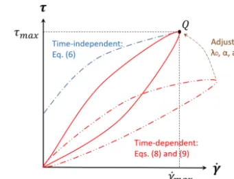
– Method B: our second approach (which is preferred) is to approximate the critical shear stress(τc)of a time-dependent fluid model using the maximum shear stress
(τmax)of a time-independent fluid model. This implies that, on a graph of stress vs. strain (τ : ˙γ), the criti-cal stress–strain point of the time-independent model should match the maximum stress point of the time-dependent model (i.e., the point where hysteresis causes the time-dependent model to operate along a different
τ : ˙γ curve). This point is labeledQin Fig. 1. It is a relatively simple graphical trial and error exercise to ad-justλ0,ω, andαto obtain the correctQfor a givenT0,
η0, andn. In this approach, the most important question is how to set the matching point, Q. In our avalanche model (Sect. 7), the pointQis known because the criti-cal shear stress is given in the experimental paper. How-ever, for our debris-flow model (Sect. 8), only time-independent parameters are given in the corresponding experimental report. Thus, the matching pointQfor this case was set where the maximum rate of strain of the thixotropic model was the same as the maximum rate of strain of the Herschel–Bulkley model.
Figure 1.Concept of a graphical method B for estimating a consis-tent set ofλ0, α, andωparameters for the Coussot model.
TheT0of the Coussot model in Eq. (10) can also be trou-blesome to estimate. This characteristic time for aging, which Coussot et al. (2002b) described as “spontaneous evolution of the microstructure”, is not widely, used and the literature does not provide insight on how to evaluateT0 as a func-tion of other rheological characteristics. Furthermore,T0has slightly different definitions by authors of several papers. Chanson et al. (2006) defined it as the characteristic time without any further measurement in their experiments, but they provided another parameter, “rest time”, used to set up the bentonite suspensions in laboratory experiments in the re-sult tables. However, Møller et al. (2006) definedT0as “the characteristic time of build-up of the microstructure at rest”. Their characteristic time is close to the rest time of Chanson et al. (2006). Therefore, we make the assumption that the rest time measured in the Chanson’s experiments is the same with theT0 of Coussot for the thixotropic avalanche simu-lations (Sect. 7). For simusimu-lations of subaqueous debris flow (Sect. 8), the experiments did not report any timescales that could be used to estimateT0, so we included it as an unknown in the method B described above. In general, the graphical method B provides a simple means to estimate a consistent set of time-dependent parameters from the time-independent parameters, which provides confidence that time-dependent and time-independent models are being compared in a rea-sonable manner.
5 Multi-material level-set method
method so that any number of fluids with differing Newto-nian and non-NewtoNewto-nian properties can be considered. When only two fluids are considered, the multi-material level-set method corresponds to the general level-set method for two-phase flow. The level-set method has a long history in multi-phase fluids (Sussman et al., 1994; Chang et al., 1996; Suss-man et al., 1998; Peng et al., 1999; SussSuss-man and Fatemi, 1999; Bovet et al., 2010) and is based on using aφi distance (level set) function to represent the distance of theimaterial (or material phase) from an interface with another material (Osher and Fedkiw, 2001).
The multi-material level-set method herein follows Merri-man et al. (1994) with the addition of high-order numerical schemes (Shu and Osher, 1989; Shi et al., 2002). The “level set” of theith fluid is designated asφi:
φi≡ (
+di(x, 0i) if xinside0i
−di(x, 0i) if xoutside0i
, (11)
wherei= {1,2,· · ·, Nm},Nmis the number of materials,0i is the interface of fluidi, anddis the distance from the inter-face. The density and viscosity at a computational node for the multiple-fluid system are evaluated from a combination of the individual fluid characteristics based on an approxi-mate Heaviside function that provides a continuous transition over somedistance on either side of an interface:
ρ≡
Nm
X
i=1
ρiHi, η≡ Nm
X
i=1
ηiHi, (12)
where the Heaviside function for fluidiis
Hi(φi)≡
0 if φi<−
1 2 h
1+φi
+ 1 πsin π φ i i
if |φi| ≤
1 if φi>
, (13)
where 2 is therefore the finite thickness of the numerical interface between fluids.
The level-set initial condition is simply the distance from any grid point in the model to an initial set of interfaces, i.e.,φi=di. Note that each point has a distance to eachi in-terface. The level set is treated as a conservatively advected variable that evolves according to a simple non-diffusive transport equation (Osher and Fedkiw, 2001):
∂φi
∂t +u· ∇φi=0. (14)
The above is coupled to a solution of momentum and con-tinuity, Eqs. (2) and (3), to form a complete level-set solu-tion for fluid flow. The continuous interface i at time t is located whereφi(x, t )=0. In general, theiinterface will be between the discrete grid points of the numerical solution, so it is found by multi-dimensional interpolation from the discrete φi values. After advancing the level set fromφ (t )
toφ (t+1t ), the values of the level set will no longer sat-isfy the eikonal condition of|∇φi| =1; that is, the level-set values on the grid cells obtained by solving Eq. (14) are no longer equidistant from the interface (i.e., the zero level set). It is known that if the level sets are naively evolved through time without satisfying the eikonal condition the Heavi-side functions will become increasingly inaccurate (Sussman et al., 1994). This problem is addressed with “reinitializa-tion”, which resets theφ (t+1t )to satisfy the eikonal condi-tion. The simplest approach to reinitialization is iterating an unsteady equation in pseudo-time to steady state such that the steady-state equation satisfies the eikonal condition (Suss-man et al., 1998). Letφˆ be an estimate of the reinitialized value forφ (t+1t )in the equation
∂φˆi
∂T +S
ˆ
φi |∇ ˆφi| −1
=0, (15)
whereT is the pseudo-time, andSis the signed function as (Sussman et al., 1998)
S(φˆi)=
−1 if φˆi<0 0 if φˆ
i=0 1 if φˆi>0
. (16)
The time-advanced set ofφ (t+1t )is the starting guess for
ˆ
φ, and the steady-state solution ofφˆwill satisfy|∇ ˆφi| =1 to numerical precision.
For the present work, the advection term in Eq. (14) is dis-cretized with the fifth-order WENO scheme, and the time-derivative term is integrated by the third-order TVD Runge– Kutta method (Shu and Osher, 1989). For the reinitializa-tion step of Eq. (15), the second-order ENO (essentially non-oscillatory) scheme (Sussman et al., 1998) and a smoothing approach (Peng et al., 1999) are used for the spatial dis-cretization (further details are provided in Jeon, 2015).
6 Poiseuille flow of Bingham fluid
A two-dimensional Poiseuille flow in a channel driven by a steady pressure gradient of∂p/∂xprovides a validation case for the non-Newtonian fluid solver. If gravity is considered negligible and the flow is approximated as symmetric about a centerline between two walls, then the analytical solution for the flow on one side of the centerline is (Papanastasiou, 1987) u(y)= 1 2η −∂p ∂x
F2−y2−
τ0
η
(F−y)
for FD≤y≤F 1 2η −∂p ∂x
F2−FD2−τ0
η
(F−FD)
for 0≤y < FD
, (17)
whereF is the distance from the center to a channel wall,y
Table 1.Bingham fluid Herschel–Bulkley model parameters used in Poiseuille flow test cases, from Filali et al. (2013).
Term Value
Herschel–Bulkley index (n) 1.0 Yield stress (τ0, Pa) 4.0 Consistency parameter (K, Pa sn) 2.9
0 at the centerline of the flow between the two walls, τ0 is the yield stress, and FD is a length scale representing the relationship between yield stress and the pressure gradient:
FD=
τ0
−∂p
∂x .
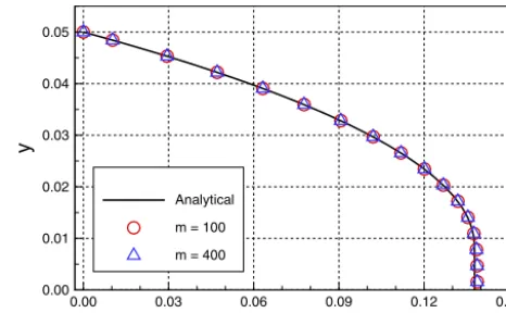
A convenient set of Bingham fluid parameters for the Poiseuille test cases can be extracted from the dip-coating study of Filali et al. (2013) as shown in Table 1. In the sim-ulations, the distance from the centerline to a side wall is 0.05 m. Our model grid uses 320 cells in the flow direc-tion and 32 cells in the cross-stream direcdirec-tion. A Neumann boundary condition is applied along the lower boundary of the simulation domain, so the simulation includes only the upper half-channel of this symmetric flow.
Using the Papanastasiou model of Eq. (6) to approximate a Herschel–Bulkley model of a Bingham fluid requires time-scale parameter m to provide smooth behavior across the yield-stress threshold. We tested values ofm= {100,400}s. As shown in Fig. 2, the numerical results are in very good agreement with the analytical solutions for both values. For this simulation, the lower value of m=100 s is reasonable for a Papanastasiou model.
7 Thixotropic avalanches
An avalanche is a granular flow of an initially solid field that is triggered from rest into a downslope flow. A thixotropic model of an avalanche as a fluid continuum can represent a rapid progression from local to global release of the ini-tial structural jamming,λ0. Chanson et al. (2006) developed dam-break experiments with a thixotropic fluid that provide reasonable facsimiles of avalanche flows if the timescale to remove the dam is smaller than the timescale for release of structural jamming. The initial conditions of the Chanson ex-periments are shown in Fig. 3 whereθ,d0, andl0represent the angle of a slope, the height of the initial avalanche that is normal to the slope, and the length of the avalanche along a slope, respectively. We modeled this same setup with our multi-material level-set solver.
The Chanson experiments identified four thixotropic flow types that were functions of the relative effect of initial struc-tural jamming. Weak jamming (i.e., small λ0) characterizes type I, such that inertial effects dominate the downstream
u
y
0.00 0.03 0.06 0.09 0.12 0.15
0.00 0.01 0.02 0.03 0.04 0.05
Analytical
m = 100
m = 400
Figure 2.Comparison of analytical and numerical solutions for steady-state fluid velocity for Poiseuille flow of a Bingham fluid.
Figure 3.Definition sketch for initial conditions of an avalanche along a slope.
flow (highest Re) and the flow only ceases when it reaches the experiment outfall. It follows that type I is effectively a model of an avalanche that propagates until it is stopped by an obstacle or change in slope. Type II flows had intermedi-ate initial jamming, which showed rapid initial flow followed by deceleration until “restructuralization”, which effectively stops the downstream progression. Type II is a model of an avalanche that dissipates itself on the slope. The type III flows, with the highestλ0, have complicated behavior with separation into identifiable packets of mass (typically two, but sometimes more) with different velocities. Type IV be-havior was the extremum of zero flow. Chanson reported 28 experiments in total, but data on wave front propagation were provided for only five experiments (Fig. 6 in Chanson et al., 2006) of type I and II behavior. We simulated three of these experiments that covered a wide range of characteris-tics and behaviors, as shown in Table 2. Note that Chanson et al. (2006) used τc2 to designate the critical shear stress during unloading (restructuralization), which we consider an approximation for the yield stress,τ0, for a time-independent model.
We simulate the three cases of Table 2 with the independent Papanastasiou model of Eq. (6) and the dependent Coussot model of Eqs. (8) and (9). For a time-independent Bingham model, we use n=1 with K=η0 from the Chanson experiments. The smoothing value of
Table 2.Dimensions and data for thixotropic avalanche simulations corresponding with experiments by Chanson et al. (2006).
Term Case 1 Case 2 Case 3
Chanson experiment no. 6 19 23
Thixotropic flow type II II I
Slope angle (θ,◦) 15 15 15
Initial height (d0, m) 0.0727 0.0756 0.0732 Initial length (l0, m) 0.2908 0.3024 0.2928 Herschel–Bulkley index (n) 1.1 1.1 1.1 Yield stress (unloading,τ0, Pa) 31.0 21.1 14.0 Critical stress (loading,τc, Pa) 90 165 50 Asymptotic viscosity (η0, Pa s) 0.062 0.635 0.555 Density (ρ, kg m−3) 1099.8 1085.1 1085.1 Characteristic (rest) time (T0, s ) 300 900 60
in Sect. 6, above. For a time-independent Herschel–Bulkley model, we use the same K and mas the Bingham plastic model, but withn=1.1 as was used in the detailed technical report on the same experiments by Chanson et al. (2004). The time-dependent model requires specification of parameters
{n, T0, α, η0, λ0, ω}as discussed in Sect. 4. The Herschel– Bulkley index in the time-dependent model uses the same value (n=1.1) as the time-independent model. Two sets of values for{α, λ0, ω}are determined by the two methods (A and B) outlined in Sect. 4, above. Method A uses Eq. (10), which requires a value for τc; herein this is taken as Chan-son’s critical loading stress (τc1in Chanson et al., 2006) dur-ing the initial structural breakdown. Similarly, method B re-quires aτmaxfor pointQin Fig. 1, which is also set to the critical loading stress.
For all simulations, the no-slip wall condition is applied to the bottom wall, and the number of computational cells is 512×80. The computational domain is rotated so thexaxis is along the sloping bed, which means that computational cell faces are either orthogonal or parallel to the slope. The gravi-tational constant (g=9.81 m s−2) is divided into two compo-nents of (gsinθ,−gcosθ). The density and viscosity of air are 1.0 kg m−3and 1.0×10⁻⁵Pa s, respectively.
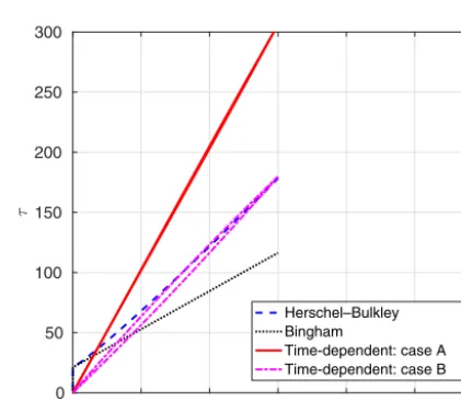
The analytical relationships between shear stress and rate of strain for the different viscosity models are presented in Figs. 4 through 6. In these figures, “Herschel–Bulkley” and “Bingham” lines are the results of Eq. (6) withn=1.1 and
n=1.0, respectively. The “case A” and “case B” lines de-note results of methods A and B from Sect. 4 for determin-ing time-dependent parameters with Eqs. (8) and (9). The es-timated parameters ofλ0,ω, andαby two methods that are used in these figures are shown in Table 3. These results illus-trate the challenge of using method A (the critical stress re-lationship) for estimatingλ0. The numerical solutions of the Coussot model ordinary differential equation, Eq. (9), are ob-tained by the Runge–Kutta fourth-order method. The result-ing time-dependent stress–strain relationship can be far from
0 100 200 300 400 500
˙ γ 0
50 100 150 200 250 300
τ
Herschel–Bulkley Bingham
Time-dependent: case A Time-dependent: case B
Figure 4.Analytical stress–strain for thixotropic avalanche case 1: shear stress (Pa) and rate of strain (s−1) withτ0=31 Pa andτc= 90 Pa. Theτaxis is scaled for comparison with Figs. 5 and 6, while theγ˙ axis has an individual scale for clarity.
0 50 100 150 200 250 300
˙
γ
0 50 100 150 200 250 300
τ
Herschel–Bulkley Bingham
Time-dependent: case A Time-dependent: case B
Figure 5.Analytical stress–strain for thixotropic avalanche case 2: shear stress (Pa) and rate of strain (s−1) withτ0=21.1 Pa andτc= 165 Pa. Theτaxis is scaled for comparison with Figs. 4 and 6, while theγ˙ axis has an individual scale for clarity.
the time-independent relationship that is otherwise thought to be a reasonable model.
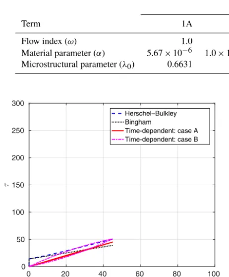
Table 3.Parameters of the time-dependent fluid model for thixotropic avalanche simulations using method A and method B for setting values.
Case
Term 1A 1B 2A 2B 3A 3B
Flow index (ω) 1.0 0.7 0.5 1.0 0.1 1.0
Material parameter (α) 5.67×10⁻⁶ 1.0×10⁻⁶ 3.56×10⁻⁶ 1.0×10⁻⁶ 5.33×10⁻⁵ 1.0×10⁻⁵ Microstructural parameter (λ0) 0.6631 0.95 3.8576 0.74 5.9235 0.29
0 20 40 60 80 100
˙ γ
0 50 100 150 200 250 300
τ
Herschel–Bulkley Bingham
Time-dependent: case A Time-dependent: case B
Figure 6.Analytical stress–strain for thixotropic avalanche case 3: shear stress (Pa) and rate of strain (s−1) withτ0=14 Pa andτc= 50 Pa. Theτaxis is scaled for comparison with Figs. 4 and 5, while theγ˙ axis has an individual scale for clarity.
was derived from equations of motion as Eq. (26) in Chanson et al. (2006), repeated here as
xs∗=sinθ
2 t
∗2
. (18)
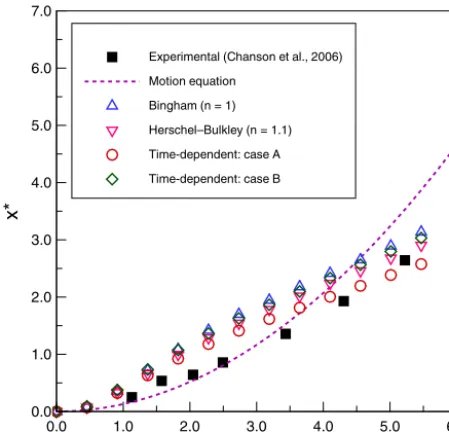
The simulation, experiment, and theory results are shown in Figs. 7, 8, and 9 for cases 1, 2, and 3 of Table 2, respectively. The dashed line represents the theoretical solution for prop-agating the front of Eq. (18).
The most striking feature in the results is that the simula-tions for cases 2 and 3 (smallerτ0) are relatively similar for all the models, whereas the time-independent models (Bing-ham and Herschel–Bulkley) completely fail for case 1 (larger
τ0) even though the time-dependent models continue to per-form reasonably well. The failure appears to be due to an inability of the time-independent models in case 1 to develop sufficient strain to move out of theη=Kγ˙n−1+mτ0regime that governs viscosity below the yield stress in Eq. (6). In contrast, the microstructural aging process that is inherent in Eqs. (8) and (9) allows the time-dependent models in case 1 to develop reasonable flow conditions despite the higherτ0.
t*
x*
0.0 1.0 2.0 3.0 4.0 5.0 6.0
0.0 1.0 2.0 3.0 4.0 5.0 6.0 7.0
Experimental (Chanson et al., 2006)
Motion equation
Bingham (n = 1)
Herschel-Bulkley (n = 1.1)
Time-dependent: case A
Time-dependent: case B
Figure 7.Thixotropic avalanche case 1: comparison of numerical results and experimental data for non-dimensional front displace-ment (x∗) as a function of non-dimensional simulation time (t∗).
No doubt the time-independent models could be made to per-form better in case 1 by further manipulation of the model coefficients; however, our approach was to use coefficients that could be set a priori based on data from the experiments and a plausiblemvalue from Sect. 6.
surpris-t*
x*
0.0 1.0 2.0 3.0 4.0 5.0 6.0
0.0 1.0 2.0 3.0 4.0 5.0 6.0 7.0
Experimental (Chanson et al., 2006)
Motion equation
Bingham (n = 1)
Herschel–Bulkley (n = 1.1) Time-dependent: case A
Time-dependent: case B
Figure 8.Thixotropic avalanche case 2: comparison of numerical results and experimental data for non-dimensional front displace-ment (x∗) as a function of non-dimensional simulation time (t∗).
t*
x*
0.0 1.0 2.0 3.0 4.0 5.0 6.0
0.0 1.0 2.0 3.0 4.0 5.0 6.0 7.0
Experimental (Chanson et al., 2006)
Motion equation
Bingham (n = 1)
Herschel-Bulkley (n = 1.1)
Time-dependent: case A
Time-dependent: case B
Figure 9.Thixotropic avalanche case 3: comparison of numerical results and experimental data for non-dimensional front displace-ment (x∗) as a function of non-dimensional simulation time (t∗).
ing that its performance degrades with increasing Reynolds number.
Although the simulations results have reasonable global agreement with experiments, on closer examination it can be seen that the 2-D simulations predict a front movement that is initially too rapid in type II flows (cases 1 and 2) and at longer times is too slow for type I flows (case 3). The
chal-lenge, of course, is that the model error is integrative: ifλis wrong at a given time, then the dλ/dt will be wrong as well and the frontal position error will accumulate. Thus, an im-portant issue for the time-dependent model appears to be se-lecting the appropriate values of{λ0, α, ω}that are consistent with experimentally determined values of{η0, τ0, τc, n, T0}. Although the more parsimonious time-independent model (with fewer parameters) performs reasonably well for our cases 2 and 3, it performs poorly in case 1 and so should only be used with caution and careful calibration.
The above observations lead to a conclusion that the accel-erative behaviors in the simulations and experiments are not well matched. The problem is shown most clearly in Fig. 7 for case 1, where the experiments initially follow the acceler-ation implied by Eq. (18) but diverge with an inflection point and deceleration occurring somewhere neart∗∼4. In con-trast, the models initially show a more rapid acceleration and an inflection point to deceleration att∗∼1. Interestingly, the simulated front locations in cases 1 and 2 are not unreason-able predictions fort∗>4, but they get there along slightly different paths than the experiments. The case 3 (type I) mod-els show different behaviors: they perform quite well for
t∗≤3 and then show deceleration at the same time as the experiment appears to be accelerating. Unfortunately, the ex-periments of Chanson et al. (2006) did not extend beyond
t∗∼6.5, so it is impossible to know whether the experiments are showing an inflection point to deceleration att∗∼5, but it seems likely given the results of the case 1 and 2 studies. If there is an inflection point for case 3, then it would appear that the consistent problem with the models is getting the correct transition from frontal acceleration to deceleration. To date, our experiments have not shown that we can signifi-cantly alter the model acceleration inflection points by alter-ing parameters, which may indicate that there is a need to fur-ther consider the fundamental forms of the Coussot and Pa-panastasiou models when used for thixotropic flows. An al-ternative explanation may be that there are three-dimensional controls on the front propagation in the experiment that can-not be represented in the present 2-D model.
8 Subaqueous debris flows
Figure 10.Submarine landslide.
0 2 4 6 8 10 12
˙ γ 0
10 20 30 40 50 60 70 80
τ
Herschel–Bulkley Time-dependent
Figure 11.Subaqueous debris case 1: shear stress (Pa) and rate of strain (s−1).
is shown in Fig. 10, with dimensions provided in Table 4. The gravitational constant for all simulations isg=9.81 m s−2.
The simulation uses 340×100 rectangular cells. The no-slip wall boundary condition is applied to the bottom bound-ary. The computational domain is rotated so thexaxis is par-allel to the slope, which allows the bottom to be represented as a straight surface without using cut grid cells or unstruc-tured grids. This rotation also provides convenience in mea-suring the variables normal to the slope (e.g., front distance and water/mud thicknesses at the front.) These simulations include three fluids: mud, water, and air. The density of mud for each case is shown in Table 6, and the densities of water and air are 1000.0 and 1.0 kg m−3, respectively.
The parameters for the time-independent fluid model from Haza et al. (2013) are shown in Table 5. For all simulations,
m=100 for the exponential smoothing parameter is used based on results from Sect. 6, above. The parameters for the time-dependent fluid model are estimated from method B in Sect. 4 and are shown in Table 6. The experiments did not report a rest time, soT0was set at a small positive value that provided a reasonable match to the experiments. The ana-lytical relationships between the shear stress and the rate of strain for the time-independent and the time-dependent fluid models are shown in Fig. 11 for case 1 and Fig. 12 for case 2. Figure 13 provides a reference for measurements used to compare the model and experiments. These include the
0 2 4 6 8 10 12
˙
γ
0 10 20 30 40 50 60 70 80
τ
Herschel–Bulkley Time-dependent
Figure 12.Subaqueous debris case 2: shear stress (Pa) and rate of strain (s−1). Axis scalings are identical to Fig. 11 for comparison purposes.
Initial position
D
H
L U
Figure 13.Run-out and head flow.
height of head flow (H), the water depth at the front of head flow (D), the run-out distance from the initial position (L), and the flow-front velocity (U). Figure 14 shows evolution of the zero level sets for water (φ2), which provides the contin-uous line separating the water from both the debris and the air. Figures 15 and 16 show the evolution of the run-out dis-tance (L) for case 1 and case 2, respectively. It can be seen that both time-independent and time-dependent models are reasonable approximations of the limited experimental data. Both types of models appear to underestimate the initial run-out and slightly overestimate later times.
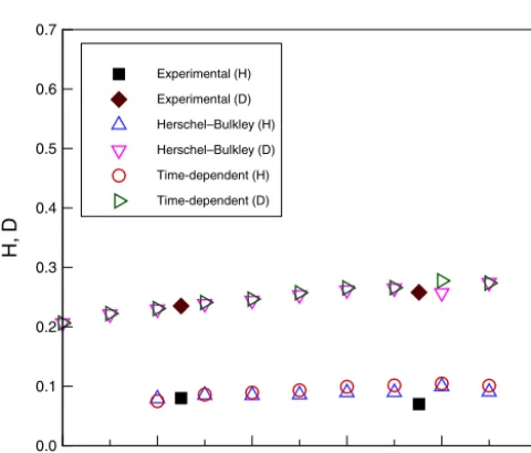
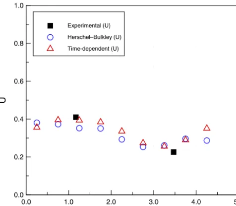
Figures 17 and 18 show a comparison ofH andD for simulations and experiments. Again, within the limited avail-ability of experimental data, both independent and time-dependent models provide reasonable agreement. Figures 19 and 20 show similar agreement for the front velocities, al-though the experimental data are insufficient to validate the wave-like oscillation of the velocity in the simulations.
x
y
0.8 1.2 1.6 2.0
0.0 0.1 0.2 0.3
Air
Water
Debris
Initial condition
Figure 14.Profiles of debris and water (φ2: water).
Table 4.Dimensions for simulations to match experiments by Haza et al. (2013).
Term Value
Angle of a slope (θ,◦) 3 Height of mud at a gate (h0, cm) 20.64 Height of mud at the end (d0, cm) 15.40 Length of mud (l0, cm) 100.0
Table 5.Parameters of the time-independent fluid model.
Term Case 1 Case 2
Herschel–Bulkley index (n) 0.5 0.42 Yield stress (τ0, Pa) 9.0 5.7 Consistency parameter (K, Pa sn) 20.36 12.68
likely a function of the experimental conditions. An impor-tant limitation of the tested subaqueous debris flows is that they do not have the restructuralization in the downstream flow or the strongly jammed initial structure seen in the ex-periments of Chanson et al. (2006)
9 Discussion and conclusions
This work shows that a multi-phase flow solver using a multi-material level-set method with yield-stress mod-els of non-Newtonian viscosity provides a means for nu-merical approximation of avalanches and subaqueous de-bris flows. This simulation approach was tested with both time-independent (Herschel–Bulkley, Papanastasiou, Bing-ham plastic) and time-dependent (thixotropic Coussot) mod-els of viscosity, which are implemented using continuum me-chanics solutions for multiple fluids. A key problem is that the Coussot model requires more parameters than the time-independent fluid models, but available experimental data are insufficient to definitively set parameter values. To resolve this issue, two different approaches were used to
evaluat-Table 6.Parameters of the time-dependent fluid model.
Term Case 1 Case 2
Density (ρ, kg m3) 1266.0 1236.0 Asymptotic viscosity (η0, Pa s) 3.12 2.1 Herschel–Bulkley index (n) 0.5 0.42
Flow index (ω) 1.0 1.0
Characteristic time (T0, s) 10.0 10.0 Material parameter (α) 1.0×10⁻⁵ 1.0×10⁻⁵ Microstructural parameter (λ0) 0.1 0.1
t
L
0.0 1.0 2.0 3.0 4.0 5.0
0.0 0.4 0.8 1.2 1.6 2.0 2.4
Experimental (L)
Herschel–Bulkley (L)
Time-dependent (L)
Figure 15.Subaqueous debris case 1: run-out distance (L, m) as a function of simulation time (t, s).
ing the Coussot parameters. Overall, the numerical results showed reasonable agreement with prior experimental data.
t
L
0.0 1.0 2.0 3.0 4.0 5.0
0.0 0.4 0.8 1.2 1.6 2.0 2.4
Experimental (L)
Herschel–Bulkley (L)
Time-dependent (L)
Figure 16.Subaqueous debris case 2: run-out distance (L, m) as a function of simulation time (t, s).
t
H,
D
0.0 1.0 2.0 3.0 4.0 5.0
0.0 0.1 0.2 0.3 0.4 0.5 0.6 0.7
Experimental (H)
Experimental (D)
Herschel–Bulkley (H)
Herschel–Bulkley (D)
Time-dependent (H)
Time-dependent (D)
Figure 17.Subaqueous debris case 1: height of head flow (H, m) and water depth (D, m) as a function of simulation time (t, s).
Bulkley and Bingham plastic models erroneously predicted near-zero flow. Nevertheless, much of the complexity in real-world behavior for debris mixtures is due to interactions across spatial scales for heterogeneous mixtures, which leads to significantly different stress–strain relationships during structural breakdown and restructuralization that should re-quire a time-dependent model. Unfortunately, for experimen-tal simplicity most researchers expend significant effort to create a homogeneous mixture as an initial condition for a debris flow, and the extent to which the structural breakdown results in temporary heterogeneous scales is unknown.
Ex-t
H,
D
0.0 1.0 2.0 3.0 4.0 5.0
0.0 0.1 0.2 0.3 0.4 0.5 0.6 0.7
Experimental (H)
Experimental (D)
Herschel–Bulkley (H)
Herschel–Bulkley (D)
Time-dependent (H)
Time-dependent (D)
Figure 18.Subaqueous debris case 2: height of head flow (H, m) and water depth (D, m) as a function of simulation time (t, s).
t
U
0.0 1.0 2.0 3.0 4.0 5.0
0.0 0.2 0.4 0.6 0.8 1.0
Experimental (U)
Herschel–Bulkley (U)
Time-dependent (U)
Figure 19. Subaqueous debris case 1: flow-front velocity (U, m s−1) as a function of simulation time (t, s).
isting laboratory data do not provide sufficiently detailed in-sight into the processes controlling destruction of jamming or the restructuralization of the flow, which leaves significant uncertainty in specification of the correct parameters.
t
U
0.0 1.0 2.0 3.0 4.0 5.0
0.0 0.2 0.4 0.6 0.8 1.0
Experimental (U)
Herschel–Bulkley (U)
Time-dependent (U)
Figure 20. Subaqueous debris case 2: flow-front velocity (U, m s−1) as a function of simulation time (t, s).
jammed structure or undergoes restructuralization as the flow slows, the time-independent Bingham plastic and Herschel– Bulkley models will likely be inadequate. Unfortunately, the processes by which the initial jamming is locally overcome, and the processes through which the structure is recovered, are both poorly understood. For time-dependent thixotropic models to be useful in modeling real-world avalanches and debris flows, there is a need for a consistent approach to defining the initial jamming (λ0), the characteristic time of aging (T0), and the asymptotic shear viscosity (η0), along with the material parametersωandαfor real-world systems. As yet, these parameters are not well defined for either sple laboratory models or comsplex real-world flows. To im-prove our understanding of the thixotropic model, there is a need for a comprehensive sensitivity analysis of these five driving parameters for the expected scales of real-world sys-tems (which are as yet unknown). Furthermore, with or with-out the thixotropic model, there is clearly a need for (1) more detailed experimental measurements during flow initiation and restructuralization, and (2) a better understanding of the relationship between measurable microstructure parameters and the effective stress–strain relationship. The present work shows that a time-dependent (thixotropic) viscosity model may be an effective proxy for representing the inception and stalling of an avalanche or debris flow, but much work re-mains to be done before real-world natural hazards can be modeled in this manner.
Data availability. The experimental data in the figures can be found in Chanson et al. (2006) and Haza et al. (2013). The simu-lation data can be obtained from the corresponding author (Chan-Hoo Jeon).
Competing interests. The authors declare that they have no conflict of interest.
Acknowledgements. The authors acknowledge the Texas Advanced Computing Center (TACC) at The University of Texas (UT) at Austin for providing HPC, visualization, database, or grid resources that have contributed to the research results reported within this paper (http://www.tacc.utexas.edu). Publication support was provided by the Center for Water and the Environment at UT Austin and the Carl Ernest and Mattie Ann Muldrow Reistle Jr. Centennial Fellowship in Engineering.
Edited by: Jean-Philippe Malet Reviewed by: two anonymous referees
References
Ancey, C.: Plasticity and geophysical flows: A review, J. Non-Newton. Fluid, 142, 4–35, 2007.
Ancey, C. and Cochard, S.: The dam-break problem for Herschel-Bulkley viscoplastic fluids down steep flumes, J. Non-Newton. Fluid, 158, 18–35, 2009.
Aziz, M., Towhata, I., Yamada, S., Qureshi, M. U., and Kawano, K.: Water-induced granular decomposition and its effects on geotechnical properties of crushed soft rocks, Nat. Hazards Earth Syst. Sci., 10, 1229–1238, https://doi.org/10.5194/nhess-10-1229-2010, 2010.
Bagdassarov, N. and Pinkerton, H.: Transient phenomena in vesic-ular lava flows based on laboratory experiments with analogue materials, J. Volcanol. Geoth. Res., 132, 115–136, 2004. Balay, S., Abhyankar, S., Adams, M. F., Brown, J., Brune, P.,
Buschelman, K., Dalcin, L., Eijkhout, V., Gropp, W. D., Kaushik, D., Knepley, M. G., McInnes, L. C., Rupp, K., Smith, B. F., Zampini, S., Zhang, H., and Zhang, H.: PETSc Web page, avail-able at: http://www.mcs.anl.gov/petsc, last access: 5 December 2016.
Balmforth, N. J. and Craster, R. V.: Geomorphological Fluid Me-chanics, in: Lecture Notes in Physics, vol. 582, Springer, Berlin, Heidelberg, Germany, 2001.
Balmforth, N. J., Craster, R. V., Rust, A. C., and Sassi, R.: Vis-coplastic flow over an inclined surface, J. Non-Newton. Fluid, 142, 219–243, 2007.
Beverly, C. R. and Tanner, R. I.: Numerical analysis of three-dimensional Bingham plastic flow, J. Non-Newton. Fluid, 42, 85–115, 1992.
Bingham, E. C.: An investigation of the laws of plastic flow, U.S. Bur. Stand. Bullet., 13, 309–353, 1916.
Bisantino, T., Fischer, P., and Gentile, F.: Rheological characteris-tics of debris-flow material in South-Gargano watersheds, Nat. Hazards, 54, 209–223, 2010.
Bovet, E., Chiaia, B., and Preziosi, L.: A new model for snow avalanche dynamics based on non-Newtonian fluids, Meccanica, 45, 753–765, 2010.
Chanson, H., Coussot, P., Jarny, S., and Toquer, L.: A Study of Dam Break Wave of Thixotropic Fluid: Bentonite Surges down an Inclined Plane, Tech. Rep. CH54/04, Department of Civil En-gineering, The University of Queensland, St. Lucia QLD, Aus-tralia, 2004.
Chanson, H., Jarny, S., and Coussot, P.: Dam break wave of thixotropic fluid, J. Hydraul. Eng., 132, 280–293, 2006. Coussot, P. and Meunier, M.: Recognition, classification and
me-chanical description of debris flows, Earth-Sci. Rev., 40, 209– 227, 1996.
Coussot, P., Nguyen, Q. D., Huynh, H. T., and Bonn, D.: Avalanche behavior in yield stress fluids, Phys. Rev. Lett., 88, 175501, https://doi.org/10.1103/PhysRevLett.88.175501, 2002a. Coussot, P., Nguyen, Q. D., Huynh, H. T., and Bonn, D.: Viscosity
bifurcation in thixotropic, yielding fluids, J. Rheol., 46, 573–589, 2002b.
Crosta, G. B. and Dal Negro, P.: Observations and modelling of soil slip-debris flow initiation processes in pyroclastic deposits: the Sarno 1998 event, Nat. Hazards Earth Syst. Sci., 3, 53–69, https://doi.org/10.5194/nhess-3-53-2003, 2003.
Darwish, M. S. and Moukalled, F.: TVD schemes for unstructured grids, Int. J. Heat Mass Tran., 46, 599–611, 2003.
Davies, T. R. H.: Large debris flows: a macro-viscous phenomenon, Acta Mech., 63, 161–178, 1986.
De Blasio, F. V., Engvik, L., Harbitz, C. B., and Elverhøi, A.: Hy-droplaning and submarine debris flows, J. Geophys. Res., 109, C01002, https://doi.org/10.1029/2002JC001714, 2004.
de Haas, T., Braat, L., Leuven, J. R. F. W., Lokhorst, I. R., and Kleinhans, M. G.: Effects of debris flow composition on runout, depositional mechanisms, and deposit morphology in laboratory experiments, J. Geophys. Res.-Earth, 120, 1949–1972, 2015. Delannay, R., Valance, A., Mangeney, A., Roche, O., and Richard,
P.: Granular and particle-laden flows: from laboratory experi-ments to field observations, J. Phys. D-Appl. Phys., 50, 053001, https://doi.org/10.1088/1361-6463/50/5/053001, 2017.
Dent, J. D. and Lang, T. E.: A viscous modified Bingham model of snow avalanche motion, Ann. Glaciol., 4, 42–46, 1983. Ferziger, J. H. and Peri´c, M.: Computational methods for fluid
dy-namics, 3rd edn., Springer, Berlin, Heidelberg, Germany, 2002. Filali, A., Khezzar, L., and Mitsoulis, E.: Some experiences with
the numerical simulation of Newtonian and Bingham fluids in dip coating, Comput. Fluids, 82, 110–121, 2013.
Guermond, J. L., Minev, P., and Shen, J.: An overview of projection methods for incompressible flows, Comput. Meth. Appl. Mech. Engrg., 195, 6011–6045, 2006.
Haza, Z. F., Harahap, I. S. H., and Dakssa, L.: Experimental studies of the flow-front and drag forces exerted by subaqueous mudflow on inclined base, Nat. Hazards, 68, 587–611, 2013.
Herschel, W. H. and Bulkley, R.: Konsistenzmessungen von Gummi-Benzollösungen, Kolloid Zeitschrift, 39, 291–300, 1926. Hewitt, D. R. and Balmforth, N. J.: Thixotropic gravity currents, J.
Fluid Mech., 727, 56–82, 2013.
Huynh, H. T., Roussel, N., and Coussot, P.: Ageing and free surface flow of a thixotropic fluid, Phys. Fluids, 17, 033101, https://doi.org/10.1063/1.1844911, 2005.
Iverson, R. M.: The physics of debris flows, Rev. Geophys., 35, 245–296, 1997.
Iverson, R. M.: The debris-flow rheology myth, in: The 3rd Interna-tional Conference on Debris-Flow Hazard Mitigation:
Mechan-ics, Prediction, and Assessment, edited by: Rickenmann, D. and Chen, C.-L., 303–314, Mills Press, Davos, Switzerland, 2003. Iverson, R. M. and Denlinger, R. P.: Flow of variably fluidized
gran-ular masses across three-dimension terrain: 1. Coulomb mixture theory, J. Geophys. Res., 106, 537–552, 2001.
Jeon, C.-H.: Modeling of Debris Flows and Induced Phenomena with Non-Newtonian Fluid Models, PhD dissertation, The Uni-versity of Texas at Austin, Austin, Texas, USA, 2015.
Jeong, S. W.: The Effect of Grain Size on the Viscosity and Yield Stress of Fine-Grained Seiments, J. Mt. Sci., 11, 31–40, 2014. Liu, K. F. and Mei, C. C.: Slow spreading of a sheet of Bingham
fluid on an inclined plane, J. Fluid Mech., 207, 505–529, 1989. Liu, W. and Zhu, K.-Q.: A study of start-up flow of thixotropic fluids
including inertia effects on an inclined plane, Phys. Fluids, 23, 013103, https://doi.org/10.1063/1.3536654, 2011.
Locat, J. and Lee, H. J.: Submarine landslides: advances and chal-lenges, Can. Geotech. J., 39, 193–212, 2002.
Malet, J. P., Remaître, A., Maquaire, O., Ancey, C., and Locat, J.: Flow susceptibility of heterogeneous marly formations: im-plications for torrent hazard control in the Barcelonnette Basin (Alpes-de-Haute-Provence, France), in: The 3rd International Conference on Debris-Flow Hazard Mitigation: Mechanics, Pre-diction, and Assessment, edited by: Rickenmann, D. and Chen, C.-L., 351–362, Mills Press, Davos, Switzerland, 2003. Manga, M. and Bonini, M.: Large historical eruptions at subaerial
mud volcanoes, Italy, Nat. Hazards Earth Syst. Sci., 12, 3377– 3386, https://doi.org/10.5194/nhess-12-3377-2012, 2012. Mei, C. C.: Lecture notes on fluid dynamics, Massachusetts Institute
of Technology (MIT), Cambridge, Massachusetts, USA, 2007. Merriman, B., Bence, J. K., and Osher, S. J.: Motion of multiple
junctions: a level set approach, J. Comput. Phys., 112, 334–363, 1994.
Mohrig, D., Elverhøi, A., and Parker, G.: Experiments on the rel-ative mobility of muddy subaqueous and subaerial debris flows and their capacity to remobilize antecedent deposits, Mar. Geol., 154, 117–129, 1999.
Moller, P., Fall, A., Chikkadi, V., Derks, D., and Bonn, D.: An at-tempt to categorize yield stress fluid behaviour, Philos. T. Roy. Soc. A, 367, 5139–5155, 2009.
Møller, P. C. F., Mewis, J., and Bonn, D.: Yield stress and thixotropy: on the difficulty of measuring yield stresses in prac-tice, Soft Matter, 2, 274–283, 2006.
Murthy, J. Y. and Mathur, S.: Periodic flow and heat transfer us-ing unstructured meshes, Int. J. Numer. Meth. Fl., 25, 659–677, 1997.
O’Brien, J. S. and Julien, P. Y.: Laboratory analysis of mudflow properties, J. Hydraul. Eng., 114, 877–887, 1988.
Osher, S. and Fedkiw, R. P.: Level set methods: An Overview and Some Recent Results, J. Comput. Phys., 169, 463–502, 2001. Papanastasiou, T. C.: Flow of materials with yield, J. Rheol., 31,
385–404, 1987.
Peng, D., Merriman, B., Osher, S., Zhao, H., and Kang, M.: A PDE-based Fast Local Level Set Method, J. Comput. Phys., 155, 410– 438, 1999.
Perret, D., Locat, J., and Martignoni, P.: Thixotropic behavior dur-ing shear of a fine-grained mud from Eastern Canada, Eng. Geol., 43, 31–44, 1996.
Pignon, F., Magnin, A., and Piau, J.: Thixotropic colloidal sus-pensions and flow curves with minimum: identification of flow regimes and rheometric consequences, J. Rheol., 40, 573–587, 1996.
Pirulli, M.: On the use of the calibration-based approach for debris-flow forward-analyses, Nat. Hazards Earth Syst. Sci., 10, 1009– 1019, https://doi.org/10.5194/nhess-10-1009-2010, 2010. Pudasaini, S. P.: A general two-phase debris flow model, J. Geophy.
Res., 117, F03010, https://doi.org/10.1029/2011JF002186, 2012. Sawyer, D. E., Flemings, P. B., Buttles, J., and Mohrig, D.: Mudflow transport behavior and deposit morphology: Role of shear stress to yield strength ratio in subaqueous experiments, Mar. Geol., 307–310, 28–39, 2012.
Scotto di Santolo, A., Pellegrino, A. M., and Evangelista, A.: Experimental study on the rheological behaviour of de-bris flow, Nat. Hazards Earth Syst. Sci., 10, 2507–2514, https://doi.org/10.5194/nhess-10-2507-2010, 2010.
Shanmugam, G.: The landslide problem, J. Palaeogeogr., 4, 109– 166, 2015.
Shi, J., Hu, C., and Shu, C.-W.: A technique of treating negative weights in WENO schemes, J. Comput. Phys., 175, 108–127, 2002.
Shu, C. W. and Osher, S.: Efficient implementation of essentially non-oscillatory shock capturing schemes II, J. Comput. Phys., 83, 32–78, 1989.
Smith, G. A. and Lowe, D. R.: Lahars: volcano-hydrologic events and deposition in the debris flow – hyperconcentrated flow con-tinuum, in: Sedimentation in Volcanic Settings, edited by: Fisher, R. V. and Smith, G. A., vol. 45, 59–70, SEPM Special Publica-tion, Tulsa, Oklahoma, USA, 1991.
Sussman, M. and Fatemi, E.: An efficient, interface-preserving level set redistancing algorithm and its application to interfacial in-compressible fluid flow, SIAM J. Sci. Comput., 20, 1165–1191, 1999.
Sussman, M., Smereka, P., and Osher, S.: A level set approach for computing solutions to incompressible two-phase flow, J. Com-put. Phys., 114, 146–159, 1994.
Sussman, M., Fatemi, E., Smereka, P., and Osher, S.: An improved level set method for incompressible two-phase flows, Comput. Fluids, 27, 663–680, 1998.