Data Censoring with Set-Membership Affine
Projection Algorithm
Hamid Reza Moradi and Akram Zardadi
Abstract
In this paper, the set-membership affine projection (SM-AP) algorithm is utilized to censor non-informative data in big data applications. To this end, the probability distribution of the additive noise signal and the excess of mean-squared error (EMSE) in steady-state are employed in order to estimate the threshold parameter of the single threshold SM-AP (ST-SM-AP) algorithm aiming at attaining the desired update rate. Furthermore, by defining an acceptable range for the error signal, the double threshold SM-AP (DT-SM-AP) algorithm is proposed to detect very large errors due to the irrelevant data such as outliers. The DT-SM-AP algorithm can censor non-informative and irrelevant data in big data applications, and it can improve misalignment and convergence rate of the learning process with high computational efficiency. The simulation and numerical results corroborate the superiority of the proposed algorithms over traditional algorithms.
Index Terms
Adaptive filtering, set-membership filtering, affine projection, data censoring, big data, outliers.
I. INTRODUCTION
D
ATA redundancy is a ubiquitous feature in machine learning and big data applications, and it results in high computational load, energy consumption, processing time, and memory usage. By exploiting data redundancy, we can improve the learning performance and reduce the computational cost. An efficient approach to exploit data redundancy is through censoring non-informative data. Indeed, there are many works in literature benefiting from data censoring, such as censoring outliers in radar data [1], big data processing [2], [3], multi-sensor systems [4], sensor-centric data reduction [5], data censoring for energy-efficient communications [6], wireless sensor networks [7], data selective adaptive filters for sparse systems [8], [9], just to name a few. These works illustrate the advantages of censoring data in comparison with utilizing all data.The set-membership filtering (SMF) is an efficient technique in dividing data into informative and non-informative data set [10]. In the SMF approach, instead of processing all data in the learning process, we evaluate, select, then process data at each iteration. Indeed, the set-membership algorithms execute a new update whenever the output estimation error is larger than a predetermined value and incoming dataset contains enough innovation. Otherwise, the set-membership approach prevents the algorithm from implementing new updates; thus we will have a reduction in the computational burden. The most well known set-membership algorithms are the set-membership normalized least-mean-square [11], [12] and the set-membership affine projection [13] algorithms, where they have the benefits of the normalized least-mean-square and the affine projection algorithms, respectively, but they decrease the computational complexity through exploiting data redundancy and censoring data. Furthermore, there are many variants of the set-membership algorithms and their applications in the literature [14]–[20].
The SMF is an efficient approach for censoring data in big data applications, whereas due to the very large amount of data it would be more practical to determine beforehand the amount/percentage of data
(H. R. Moradi) YOUNG RESEARCHERS AND ELITE CLUB, MASHHAD BRANCH, ISLAMIC AZAD UNIVERSITY, MASHHAD, IRAN.
E-mail address: [email protected].
(A. Zardadi) DEPARTMENT OF MATHEMATICS, PAYAME NOOR UNIVERSITY (PNU), P.O. Box, 19395-4697, TEHRAN, IRAN. E-mail address: [email protected].
2010 Mathematics Subject Classification: 68T05, 68Q32, 68W27.
we desire to use in the learning process. In real applications, many restrictions can affect our ability to analyze the incoming data, such as limitations on available energy, time, memory, etc. Therefore, to surmount the restrictions and obtain the desired performance, we should be able to determine the informative incoming data. In this paper, we use the desired probability of updating of parameters in order to estimate the threshold parameter in the single threshold set-membership affine projection (ST-SM-AP) algorithm. Indeed, the function of the threshold parameter in the SM-AP algorithm is to censor non-informative data, thus estimating this parameter is crucial to censor data properly.
The set-membership algorithms, including the ST-SM-AP, censor incoming data based on the energy of the error signal. Indeed, if the energy of the error signal is larger than the threshold parameter, the ST-SM-AP algorithm will update the coefficients of the adaptive filter; otherwise they will remain unchanged. However, very high errors do not always show the presence of informative data. More precisely, sometimes we observe very high error signal because of the existence of some irrelevant data such as outliers and, in these cases, censoring data is more practical. Hence, we propose the double threshold set-membership affine projection (DT-SM-AP) algorithm which considers an acceptable range for the absolute value of the error signal to censor non-informative and irrelevant data and to prevent unnecessary updates. The DT-SM-AP algorithm implements the update whenever the absolute value of the error signal is between two threshold parameters [21].
This paper is organized as follows. Section II reviews the ST-SM-AP algorithm. Section III proposes the estimate of the threshold parameter in order to censor non-informative incoming data. The DT-SM-AP algorithm is introduced in Section IV. Simulations and conclusions are presented in Sections V and VI, respectively.
Notations: Scalars are denoted by lower case letters. Vectors (matrices) are represented by lowercase (uppercase) boldface letters. At iteration k, the optimum solution, the weight vector, and the input vector are denoted by wo, w(k), x(k) ∈ RN+1, respectively, where N is the adaptive filter order. For a given
iteration k, the error signal is defined as e(k),d(k)−wT(k)x(k), where d(k)∈ Ris the desired signal
and (·)T stands for the vector and matrix transposition. Moreover, P[·] and E[·] denote the probability
and the expected value operators, respectively.
II. THESINGLE THRESHOLD SET-MEMBERSHIP AFFINE PROJECTION ALGORITHM
By taking advantage of old data, data-reusing algorithms can improve the convergence rate of the learning process, particularly when the input signal is correlated. The affine projection (AP) algorithm has been traditionally considered as the benchmark among data-reusing algorithms; however, the AP algorithm is not capable of exploiting data redundancy. By incorporating the set-membership technique to the AP algorithm, the single threshold set-membership affine projection (ST-SM-AP) algorithm has already been introduced [13] in order to reduce the computational burden of the AP algorithm. However, we intend to utilize the ST-SM-AP algorithm in order to censor data and exploit data redundancy in big data applications. First, let us define some necessary variables for the ST-SM-AP algorithm. Suppose that x(k) and d(k) are the input vector and the desired signal, respectively, and the last L+ 1 input vectors and desired signals are available. For a given iteration k, suppose that the input matrix X(k), the input vectorx(k), the adaptive filterw(k), the desired vectord(k), the additive noise vectorn(k), the constraint vector (CV) γ(k), and the error vector e(k) are described as follows
X(k) = [ x(k) x(k−1) · · · x(k−L) ] ∈ R(N+1)×(L+1),
x(k) = [ x(k) x(k−1) · · · x(k−N) ]T ∈ RN+1,
w(k) = [ w0(k) w1(k) · · · wN(k) ]T ∈ RN+1,
d(k) = [ d(k) d(k−1) · · · d(k−L) ]T ∈ RL+1,
n(k) = [ n(k) n(k−1) · · · n(k−L) ]T ∈ RL+1,
γ(k) = [ γ0(k) γ1(k) · · · γL(k) ]T ∈ RL+1,
e(k) = [ e0(k) e1(k) · · · eL(k) ]T ∈ RL+1,
where N and L are the adaptive filter order and the data-reuse factor, respectively. The entries of γ(k)
should satisfy |γi(k)| ≤γ1, for i = 0,1,· · ·, L, where γ1 ∈R+ is the upper bound for the magnitude of
the error signal. Moreover, The error vector e(k) is defined as e(k) =d(k)−XT(k)w(k). We can now represent the recursion rule of the ST-SM-AP algorithm by [13]
w(k+ 1) =
(
w(k) +X(k)
h
XT(k)X(k) +δI
i−1
(e(k)−γ(k)) if |e(k)|> γ1,
w(k) otherwise,
(2)
where δ ∈R+ and I ∈R(L+1)×(L+1) are a regularization factor and the identity matrix, respectively, and
δI is added to XT(k)X(k) in order to avoid numerical problems in the matrix inversion. In the following
section, we intend to introduce an approach to estimate γ1 such that it leads to the desired update rate in big data applications.
III. ESTIMATINGγ1 IN THE ST-SM-AP ALGORITHM
In this section, we obtain an estimate for γ1 in the ST-SM-AP algorithm for online censoring in streaming big data applications. In the presence of data redundancy and streaming data, it is desirable to obtain an acceptable solution by using a predetermined percentage of data instead of processing all received data. The percentage of data we want to use gives us the update rate of the ST-SM-AP algorithm. Therefore, for a given predetermined update rate, we intend to estimate the thresholdγ1 so that the update rate of the ST-SM-AP algorithm does not exceed the predetermined update rate. In other words, for a given 0< p <1 and considering Equation (2), we intend to estimate γ1 such that
P[|e(k)|> γ1] =p. (3)
In the above equation, the predetermined update rate prepresents the percentage of data we would like to utilize in the learning process. Note that the responsibility of γ1 is to choose the most informative data, by considering p, for the learning process.
If we know the probability distribution of the error signal e(k), then we can calculate the suitable value of γ1. Generally, we do not have access to the probability distribution of the error signal; however, when the adaptive filter order is sufficiently large, the error signal e(k) and the additive noise signaln(k) have the same probability distribution in the steady-state. Therefore, by utilizing the probability distribution of
n(k) in (3), we will be able to calculate the proper value of γ1.
Note that the error signal e(k) is obtained by subtracting the output of the adaptive filter from the desired signal, thus we have
e(k) =d(k)−xT(k)w(k) = xT(k)wo+n(k)−xT(k)w(k) =xT(k)[wo−w(k)]T +n(k) =ee(k) +n(k),
(4)
whereee(k)is the noiseless error signal. Furthermore, we know that the ST-SM-AP algorithm is robust [22], thus kE[wo −w(k)]k2 < ∞, for all k ∈ N. It means that the ST-SM-AP algorithm never diverges. In
general, we have E[wo−w(k)]≈0 in the steady-state, where 0 stands for the zero vector.
A notable example for the probability distribution of the additive noise signal is the zero-mean Gaussian noise with varianceσn2. Therefore, assuming this important case, we are capable of estimating the threshold
γ1. As we know, the noiseless error signal ee(k) is uncorrelated with the additive noise signal n(k), thus using (4) we get
E[e(k)] = E[ee(k)] + E[n(k)] = 0, (5)
Var[e(k)] = E[ee2(k)] +σn2. (6)
The value ofE[ee2(k)]is called the excess of mean-squared error (EMSE), and for the ST-SM-AP algorithm
in the steady-state is described by [23]
E[ee2(k)] = (L+ 1)[σ
2
n+γ21−2γ1σ2nρ]p
[(2−p)−2(1−p)γ1ρ]
1−a
1−aL+1
where
ρ=
s
2
π(2σ2
n+ L+11 γ 2 1)
, (8)
a= [1−p+ 2pγ1ρ](1−p). (9)
As can be seen in Equation (7), in order to compute E[ee2(k)] we need γ1, whereas our target is to
estimate γ1. Therefore, initially, in the steady-state, we consider that the value ofE[ee2(k)]is equal to zero
and the distribution of e(k) is identical to the distribution of n(k). It means that, for the first moment,
E[e(k)] = 0, Var[e(k)] = σn2, and the distribution of e(k) is the zero-mean Gaussian with variance σ2n.
Thus for a given p, using the relation (3), we can compute the initial estimate of γ1. In other words, we have
P[|e(k)|> γ1] = P[e(k)<−γ1] + P[e(k)> γ1] =p, (10)
since the Gaussian distribution is symmetric, we get
P[e(k)> γ1] = p
2. (11)
Hence, we should compute γ1 by equation
Z ∞
γ1
1
p
2πσ2
n
exp(− r
2
2σ2
n
)dr = p
2, (12)
where exp(·) stands for the exponential function. Thus, for a given update rate p, we can find the initial estimate of γ1 using the standard normal distribution table.
Then, by having the initial estimate of γ1 at hand, we should replace it in Equations (7), (8), and (9) to calculate E[ee2(k)]. Ultimately, by having E[ee2(k)], we will compute the variance of e(k) utilizing Equation (6). Thus, the distribution of the error signal is the zero-mean Gaussian with variance σe2 =
Var[e(k)] = E[ee2(k)] +σ2n and, by utilizing this distribution probability, we can attain a better estimate
for γ1. Indeed, the estimate of γ1 can be obtained from equation
Z ∞
γ1
1
p
2πσ2
e
exp(− r
2
2σ2
e
)dr= p
2, (13)
where we can achieve the new estimate of γ1 by standard normal distribution table. we should remind that the selected update rate p describes a loose relative importance of the innovation caused by the new incoming input and desired data set.
IV. THE DOUBLE THRESHOLD SET-MEMBERSHIP AFFINE PROJECTION ALGORITHM
In the previous section, a process to estimate the threshold parameter of the ST-SM-AP algorithm has been addressed such that the update rate of the algorithm does not exceed a predetermined value p. The ST-SM-AP algorithm avoids updating the adaptive filter parameters when the absolute value of the error signal is less than γ1. Indeed, the ST-SM-AP algorithm assumes all incoming data set with absolute value error larger than γ1 as innovative information; however, this is not always true, particularly in the presence of outliers. In this section, we intend to introduce the double threshold set-membership affine projection (DT-SM-AP) algorithm to censor non-informative data and exploit data redundancy, also to avoid outliers effect, acquisition system saturation, and impulsive noise.
For a given iteration k, the ST-SM-AP algorithm updatew(k)if|e(k)|> γ
1, i.e., it updatesw(k)when
filter coefficients. To this end, we recommend to define an acceptable range for the absolute value of the error signal and to adopt a lower threshold γ1 and an upper thresholdγ2. Then, at each iterationk, if the incoming data set results in an error e(k) such that γ1 <|e(k)|< γ2, we implement a new updates since it means that the incoming data set brought about some innovation; otherwise we avoid new update since the incoming data brought about non-innovative or irrelevant information.
Finally, the update equation of the DT-SM-AP algorithm can be given by
w(k+ 1) =
(
w(k) +X(k)
h
XT(k)X(k) +δIi−1(e(k)−
γ(k)) if γ1 <|e(k)|< γ2,
w(k) otherwise.
(14)
The task of γ1 is to ignore the incoming data set without enough innovation, thus we can utilize the strategy described in the previous section in order to estimateγ1. However, γ2 is responsible for detecting irrelevant incoming data set, such as outliers, thus depending on the applications we should adopt a large enough value for γ2.
V. SIMULATIONS
In this section, we have applied the AP, the ST-SM-AP and DT-SM-AP algorithms to a system identification problem. For the ST-SM-AP algorithm, the threshold parameter γ1 is estimated employing the strategy explained in Section III in order to update the ST-SM-AP algorithm with the desired update rate p. The unknown systemwo has 10 coefficients, and they are drawn from the normal distribution. We have tested the results for three different input signals, namely binary phase-shift keying (BPSK), zero-mean white Gaussian noise with unit variance (WGN), and the first-order autoregressive signal (AR(1)) produced by x(k) = 0.95x(k −1) +m(k), where m(k) is a WGN signal. The signal-to-noise ratio is 20 dB; i.e., the additive noise signal has variance σn2 = 0.01. The regularization parameter δ is set to be
10−12, and the initialization for the adaptive filter is adopted as w(0) = [0 · · · 0]T. The constraint vector
(CV) is selected as the simple choice CV [22]. The simple choice CV is defined as γ0(k) =γ1
e(k)
|e(k)| and
γi(k) = ei(k) for i= 1,· · · , L. Moreover, the step-size parameter for the AP algorithm is represented at
the legend of each figure. The number of iterations is 5×10⁴, and the learning curves and the update
rates are the averages of outcomes of 100 independent ensembles.
A. Scenario 1
In this scenario, we have utilized the estimated threshold parameter γ1 in the ST-SM-AP algorithm in order to achieve the desired results by the given update rates p = 0.15, 0.30, and 0.45. The estimated threshold parameters for L = 0,1,2,3,4 and p = 0.15, 0.30, 0.45 are obtained by using the argument described in Section III, and they are listed in Table I. Furthermore, the update rates of the ST-SM-AP algorithm using these threshold parameters and different input signals in 5×10⁴ iterations are presented
TABLE I
THE VALUE OF ESTIMATEDγ1FOR DIFFERENT VALUES OFpANDL
❍ ❍
❍ ❍❍
p L 0 1 2 3 4
0.15 0.1661 0.1692 0.1716 0.1736 0.1753 0.30 0.1199 0.1222 0.1244 0.1266 0.1292 0.45 0.0871 0.0900 0.0962 0.0998 0.1037
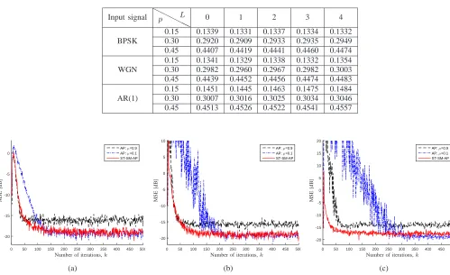
TABLE II
THE RESULTING UPDATE RATES USING THE ESTIMATEDγ1FOR DIFFERENT VALUES OFpANDLFOR THEST-SM-APALGORITHM WITH DIFFERENT INPUT SIGNALS
Input signal ❍
❍ ❍
❍❍
p L 0 1 2 3 4
BPSK
0.15 0.1339 0.1331 0.1337 0.1334 0.1332 0.30 0.2920 0.2909 0.2933 0.2935 0.2949 0.45 0.4407 0.4419 0.4441 0.4460 0.4474
WGN
0.15 0.1341 0.1329 0.1338 0.1332 0.1354 0.30 0.2982 0.2960 0.2967 0.2982 0.3003 0.45 0.4439 0.4452 0.4456 0.4474 0.4483
AR(1)
0.15 0.1451 0.1445 0.1463 0.1475 0.1484 0.30 0.3007 0.3016 0.3025 0.3034 0.3046 0.45 0.4513 0.4526 0.4522 0.4541 0.4557
0 50 100 150 200 250 300 350 400 450 500 -20 -15 -10 -5 0 AP: µ=0.9 AP: µ=0.1 ST-SM-AP PSfrag replacements M S E [d B ]
Number of iterations,k
(a)
0 50 100 150 200 250 300 350 400 450 500 -20 -15 -10 -5 0 5 10 AP: µ=0.9 AP: µ=0.1 ST-SM-AP PSfrag replacements M S E [d B ]
Number of iterations,k
(b)
0 50 100 150 200 250 300 350 400 450 500 -20 -15 -10 -5 0 5 10 15 20 AP: µ=0.9 AP: µ=0.1 ST-SM-AP PSfrag replacements M S E [d B ]
Number of iterations,k
(c)
Fig. 1. The MSE learning curves of the AP and the ST-SM-AP algorithms forL= 2andγ
1= 0.1716considering: (a) BPSK input signal;
(b) WGN input signal; (c) AR(1) input signal.
for small step-size the AP algorithm can attain the same MSE of the ST-SM-AP algorithm; however, the convergence rate of the AP algorithm degrades significantly. Therefore, the ST-SM-AP algorithm can reach low MSE with a high convergence rate as compared to the AP algorithm. Furthermore, it is worth mentioning that the ST-SM-AP algorithm has extremely lower computational complexity in comparison with the AP algorithm since it censors non-informative incoming data and avoids unnecessary updates, whereas the AP algorithm updates the adaptive filter coefficients at every iteration. Hence, the ST-SM-AP algorithm has the great potential to reduce the computational burden in big data applications.
B. Scenario 2
TABLE III
THE RESULTING UPDATE RATES USING THE ESTIMATEDγ1S ANDγ2 = 1FOR DIFFERENT VALUES OFpANDLFOR THEDT-SM-AP
ALGORITHM WITH DIFFERENT INPUT SIGNALS
Input signal ❍
❍ ❍
❍❍
p L 0 1 2 3 4
BPSK
0.15 0.1347 0.1342 0.1348 0.1341 0.1339 0.30 0.2943 0.2934 0.2941 0.2944 0.2951 0.45 0.4426 0.4435 0.4448 0.4473 0.4472
WGN
0.15 0.1352 0.1351 0.1349 0.1357 0.1363 0.30 0.2973 0.2966 0.2974 0.2989 0.2996 0.45 0.4448 0.4454 0.4469 0.4475 0.4487
AR(1)
0.15 0.1459 0.1452 0.1458 0.1471 0.1486 0.30 0.29992 0.3009 0.3015 0.3026 0.3034 0.45 0.4507 0.4518 0.4514 0.4529 0.4540
multiplying uniformly distributed random numbers belong to the interval (0,50). For the DT-SM-AP algorithm, we adopt γ2 = 1 in order to detect outliers and avoid updating adaptive filter coefficients for irrelevant incoming data. By utilizing the threshold parameters γ1s presented in Table I and γ2 = 1, the update rates of the DT-SM-AP algorithm for different data reuse factors L and different input signals are given in Table III. Similarly to Scenario 1, we can observe that in the presence of outliers signal, by utilizing the estimatedγ1s, for all input signals the resulting update rates are given in Table III are close to the given value of p. Indeed, the DT-SM-AP algorithm detected outliers signal and non-informative data effectively and avoided unnecessary updates when receiving insignificant and irrelevant incoming data. It is worthwhile to notice that, in Table III, the difference between the values of resulting update rates and their corresponding values of p is less than 0.02 (2 percent); therefore, it shows that the estimated γ1s and γ2 have censored the incoming data as we wanted.
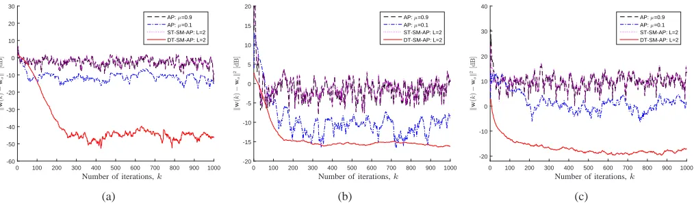
Furthermore, Figures 2(a), 2(b), and 2(c) illustrate the misalignment curves of the AP, the ST-SM-AP, and the DT-SM-AP algorithms for the BPSK, WGN, and AR(1) input signals, respectively. For all mentioned algorithms, the data reuse factor Lis selected to be 2. Also, the desired update rate isp= 0.15, therefore, the estimated γ1 is adopted equal to 0.1716 as given in Table I, and γ2 = 1 in order to detect outliers and avoid unnecessary updates. Similarly to Scenario 1, we have adopted two step-sizes 0.1 and 0.9 in the AP algorithm, so that the small step-size results in low MSE and low convergence rate but the large step-size leads to high MSE and high convergence speed. In Figures 2(a), 2(b), and 2(c), the update rates of the DT-SM-AP algorithm are 0.1348, 0.1349, and 0.1458, respectively, as described in Table III; however, the update rates of the ST-SM-AP algorithm are high values 0.8692, 0.8734, and 0.8985, respectively, because of unnecessary updates in the presence of outliers. As can be seen in these figures, the AP algorithm using neither large nor small step-sizes can reach the misalignment of the DT-SM-AP algorithm. Moreover, the misalignment and convergence speed of the ST-DT-SM-AP algorithm are the same as those of the AP algorithm using the large step-size 0.9. Therefore, in the presence of outliers, neither ST-SM-AP nor AP algorithms can attain the superb performance of the DT-SM-AP algorithm. Indeed, in the presence of outliers, the DT-SM-AP algorithm outperforms the ST-SM-AP and the AP algorithms by obtaining lower misalignment, lower update rate, and higher convergence rate.
VI. CONCLUSIONS
0 100 200 300 400 500 600 700 800 900 1000 k w ( k ) − w o k 2[d B ] -60 -50 -40 -30 -20 -10 0 10 20 30
AP: µ=0.9 AP: µ=0.1 ST-SM-AP: L=2 DT-SM-AP: L=2
PSfrag replacements
MSE [dB]
Number of iterations,k
(a)
0 100 200 300 400 500 600 700 800 900 1000
k w ( k ) − w o k 2[d B ] -20 -15 -10 -5 0 5 10 15 20
AP: µ=0.9 AP: µ=0.1 ST-SM-AP: L=2 DT-SM-AP: L=2
PSfrag replacements
MSE [dB]
Number of iterations,k
(b)
0 100 200 300 400 500 600 700 800 900 1000
k w ( k ) − w o k 2[d B ] -20 -10 0 10 20 30 40
AP: µ=0.9 AP: µ=0.1 ST-SM-AP: L=2 DT-SM-AP: L=2
PSfrag replacements
MSE [dB]
Number of iterations,k
(c)
Fig. 2. The misalignment curves of the AP, the ST-SM-AP, and the DT-SM-AP algorithms forL= 2,γ1= 0.1716, andγ2= 1considering: (a) BPSK input signal; (b) WGN input signal; (c) AR(1) input signal.
value of the output estimation error is smaller than the estimated threshold. However, the two thresholds in the DT-SM-AP algorithm prevent the algorithm from updating adaptive filter parameters when the absolute value of the error signal is outside the range defined by the thresholds. The numerical results indicate that the ST-SM-AP and the DT-SM-AP algorithms outperform the conventional affine projection algorithm.
REFERENCES
[1] S. Han, S. De Maio, V. Carotenuto, L. Pallotta, and X. Huang, “Censoring outliers in radar data: an approximate ML approach and its analysis,” IEEE Transactions on Aerospace and Electronic Systems, pp. 1–1, July 2018.
[2] P.S.R. Diniz and H. Yazdanpanah, “Data censoring with set-membership algorithms,” in IEEE Global Conference on Signal and Information Processing (GlobalSIP 2017), Montreal, Canada, November 2017, pp. 121–125.
[3] H. Zhu, H. Qian, X. Luo, and Y. Yang, “Adaptive queuing censoring for big data processing,” IEEE Signal Processing Letters, vol. 25, no. 5, pp. 610–614, May 2018.
[4] Y. Zheng, R. Niu, and P.K. Varshney, “Sequential bayesian estimation with censored data for multi-sensor systems,” IEEE Transactions on Signal Processing, vol. 62, no. 10, pp. 2626–2641, May 2014.
[5] E.J. Msechu and G.B. Giannakis, “Sensor-centric data reduction for estimation with WSNs via censoring and quantization,” IEEE Transactions on Signal Processing, vol. 60, no. 1, pp. 400–414, January 2012.
[6] J. Fern´andez-Bes, R. Arroyo-Valles, and J. Cid-Sueiro, “Cooperative data censoring for energy-efficient communications in sensor networks,” in IEEE International Workshop on Machine Learning for Signal Processing, Santander, Spain, September 2011, pp. 1–6. [7] E.J. Msechu and G.B. Giannakis, “Decentralized data selection for MAP estimation: a censoring and quantization approach,” in 14th
International Conference on Information Fusion, Chicago, IL, USA, July 2011, pp. 1–8.
[8] H. Yazdanpanah, P.S.R. Diniz, and M.V.S. Lima, “A simple set-membership affine projection algorithm for sparse system modeling,” in 24th European Signal Processing Conference (EUSIPCO 2016), Budapest, Hungary, September 2016, pp. 1798–1802.
[9] H. Yazdanpanah and P.S.R. Diniz, “Recursive least-squares algorithms for sparse system modeling,” in IEEE International Conference on Acoustics, Speech and Signal Processing (ICASSP 2017), New Orleans, LA, USA, March 2017, pp. 3879–3883.
[10] P.S.R. Diniz, Adaptive Filtering: Algorithms and Practical Implementation, Springer, New York, USA, 4th edition, 2013.
[11] S. Gollamudi, S. Nagaraj, S. Kapoor, and Y.-F. Huang, “Set-membership filtering and a set-membership normalized LMS algorithm with an adaptive step size,” IEEE Signal Processing Letters, vol. 5, no. 5, pp. 111–114, May 1998.
[12] S. Gollamudi, S. Kapoor, S. Nagaraj, and Y.-F. Huang, “Set-membership adaptive equalization and updator-shared implementation for multiple channel communications systems,” IEEE Transactions on Signal Processing, vol. 46, no. 9, pp. 2372–2385, September 1998. [13] S. Werner and P.S.R. Diniz, “Set-membership affine projection algorithm,” IEEE Signal Processing Letters, vol. 8, no. 8, pp. 231–235,
August 2001.
[14] H. Yazdanpanah and P.S.R. Diniz, “New trinion and quaternion set-membership affine projection algorithms,” IEEE Transactions on Circuits and Systems II: Express Briefs, vol. 64, no. 2, pp. 216–220, February 2017.
[15] P.S.R. Diniz and H. Yazdanpanah, “Improved set-membership partial-update affine projection algorithm,” in IEEE International Conference on Acoustics, Speech and Signal Processing (ICASSP 2016), Shanghai, China, March 2016, pp. 4174–4178.
[16] N. Takahashi and I. Yamada, “Steady-state mean-square performance analysis of a relaxed set-membership NLMS algorithm by the energy conservation argument,” IEEE Transactions on Signal Processing, vol. 57, no. 9, pp. 3361–3372, September 2009.
[17] M.Z.A. Bhotto and A. Antoniou, “A robust constrained set-membership affine-projection adaptive-filtering algorithm,” IEEE Transac-tions on Signal Processing, vol. 60, no. 1, pp. 73–81, January 2012.
[18] J.R. Deller, “Set-membership identification in digital signal processing,” IEEE ASSP Magazine, vol. 6, no. 4, pp. 4–20, October 1989. [19] S. Nagaraj, S. Gollamudi, S. Kapoor, and Y.-F. Huang, “BEACON: an adaptive set-membership filtering technique with sparse updates,”
[20] H. Yazdanpanah, M.V.S. Lima, and P.S.R. Diniz, “On the robustness of the set-membership NLMS algorithm,” in 9th IEEE Sensor Array and Multichannel Signal Processing Workshop (SAM 2016), Rio de Janeiro, Brazil, July 2016, pp. 1–5.
[21] P.S.R. Diniz, R.P. Braga, and S. Werner, “Set-membership affine projection algorithm for echo cancellation,” in International Symposium on Circuits and Systems (ISCAS 2006), Island of Kos, Greece, May 2006.
[22] H. Yazdanpanah, M.V.S. Lima, and P.S.R. Diniz, “On the robustness of set-membership adaptive filtering algorithms,” EURASIP Journal on Advances in Signal Processing, vol. 72, pp. 1–12, December 2017.