Preference Neural Network
Ayman Elgharabawy
, Mukesh Prasad
Senior Member,
IEEE
, Nikhil R. Pal
, Fellow
IEEE
, Chin-Teng
Lin
, Fellow
IEEE
Abstract—Equality and incomparability multi-label ranking have not been introduced to learning before. This paper proposes new native ranker neural network to address the problem of multi-label ranking including in-comparable preference orders using a new activation and error functions and new architecture. Preference Neural
Network PNN solves the multi-label ranking problem,
where labels may have indifference preference orders
or subgroups which are equally ranked. PNN is a
non-deep, multiple-value neuron, single middle layer and one or more output layers network. PNN uses a novel
positive smooth staircase (PSS) or smooth staircase (SS)
activation function and represents preference orders and Spearman ranking correlation as objective functions. It
is introduced in two types, Type A is traditional NN
architecture and Type B uses expanding architecture by introducing new type of hidden neuron has multiple activation function in middle layer and duplicated output layers to reinforce the ranking by increasing the number
of weights. PNN accepts single data instance as inputs
and output neurons represent the number of labels and
output value represents the preference value. PNN is
evaluated using a new preference mining data set that contains repeated label values which have not
experi-mented on before. SS and PS speed-up the learning and
PNN outperforms five previously proposed methods for
strict label ranking in terms of accurate results with high computational efficiency.
Index Terms—Preference learning, Multi-label ranking, Neural network, Kendall’s tau, Preference mining
I. INTRODUCTION
P
REFERENCE learning (PL) is emerging as anex-tended paradigm in machine learning by inducing predictive preference models from experimental data [?] [?] [?].PLhas applications in a variety of research areas such as knowledge discovery and recommender systems [?]. Objects, instances and label ranking are the three main categories of PL. Of those, label ranking (LR) is a challenging problem that has gained importance in information retrieval by search engine [?] [?]. Unlike the standard problems of regression and classification, multi-label ranking involves predicting the relation between the orders of multiple labels. In case of multiclass classifica-tion, for a given instance x from the instance space x, there is a label yassociated with x, where y∈ L, where
L= {λ1,..,λn}, where n is the number of labels. LR is an extension of multi-class and multi-label classification, where each instance x is assigned an ordering of all the class labels in the setL. This ordering gives the ranking of the labels for the given object x. This ordering can be represented by a permutation of the set {1, 2,· · ·,n}. The label order has the following three features. Irreflex-ive where λa λa ,Transitive where λaÂλb ∧ λbÂλc
=⇒ λaÂλc and Asymmetric λaÂλb then λbλa. Label preference takes one of two forms, Strict and Non-Strict order. The strict label order (λaÂλbÂλcÂλd) can be rep-resented as π=(1,2,3,4) and for non-restricted total order
π=(λaÂλb'λcÂλd) can be represented as π=(1, 2, 2, 3), where a, b, c and d are the label indexes and λa, λb, λc andλd are the ranking values of these labels respectively. For the non-continuous permutation space, The order can be represented by the aforementioned relations in addition to the incomparability binary relation ⊥. For example the partial order λaÂλbÂλd can be represented asπ=(1,2,0,3) where 0 represents an incomparable relation since λc is not comparable to (λa,λb,λd)
Various label ranking methods have been introduced in recent years [?]such as Decomposition based methods, Sta-tistical methods, Similarity and Ensemble based methods. Decomposition methods include pairwise comparison [?] [?], log linear models and constraint classification [?]. The pairwise approach introduced by hüllermeier [?] divides the multi-label ranking problem into several binary clas-sification problems in order to predict the pairs of labelsλi Âλj orλj≺λiforan inputx. Statistical methods includes decision trees [?], instance based methods (Plackett-Luce) [?] and Gaussian mixture model [?] based approaches.For example, [?] use Gaussian Mixture models to learn soft pairwise label preferences. Similarity methods minimize the labels distance instead of maximizing the probability of label values. For example, Aiguzhinov et al. [?] used an adapted version of Naive Bayes algorithm which used similarity between label rankings instead of probability. Association rules mining has also been adapted for label ranking [?]. The multilayer perceptron has also been adapted for label ranking [?], [?]. For example, in [?] six approaches are proposed that use label ranking loss during back propagation.
Instance-based decision tree was introduced by Cheng and Hüllermeier to rank the labels based on predictive probability models of a decision tree [?]. Hüllermeier combined both a decision tree and supervised clustering in two approaches for label ranking by mapping between instances and multi-labels ranking space [?].
Neural Networks (NN) for ranking were first introduced as (RankNet) by Burge to solve the problem of object ranking for sorting web documents by search engine [?]. Rank-net uses Gradient descent and probabilistic ranking cost function for each object pair. Multilayer perceptron (MLP-LR) for label ranking [?] employs NN architecture using sigmoid activation function to calculate the error between the actual and expected values of the output labels. However, It uses local approach it minimizes the
dividual error per each output neuron by subtract actual -predicted value and uses Kendall error as global approach. Both approaches doesn’t use ranking objective function in BP and learning steps. Zhou and Yangming provided a scalable decision tree structure by implementing a ran-dom forest with a parallel computational architecture for extreme label ranking [?]. Claudio Rebelo introduced label random forest (LRF) as an ensemble method of ranking [?].LRFwas based on the best approach result of previous ranking decision trees using entropy-based ranking. Jung and Tewari proposed an approach for label ranking based on voting of the best learners and scoring the labels for
ranking [?]. Song and Huang proposed a framework to
solve the vulnerability of multi-label deep learning models
[?]. Yan and Wang proposed a long short term memory
(LSTM) based multi-label ranking model for document classification [?]. This method uses a twostep process -the first step learns -the document representation while -the second step ranks the labels. Guo and Hou introduced low rank multi-label classification with missing labels (LRML) which recovered the missing labels via Laplacian manifold regularization derived from the feature space by utilizing
the low-rank mapping [?]. In our study we shall use
stair-case activation functions. In this context it is worth noting that Staircase activation function has been used for rule extraction from a multi-layer perceptron network [?]. Moraga and Heider [?] proposed a Generalized Multi-pleâ ˘A ¸Svalued Neuron with a differentiable soft staircase activation function which is represented by a sum of a set of sigmoidal functions.
Some of the above mentioned methods and their vari-ants have some issues which can be broadly categorized into two types:
(i) Drawbacks of classification based models: When the ranking model is constructed using binary classifi-cation models of an associated higher dimensional label space, such a method cannot take into account interaction between labels. In this case such rankings based on minimizing pairwise classification error is not necessarily equivalent to maximizing the perfor-mance of the label ranking considering all labels. (ii) Drawbacks of Probability based models: Some such
methods use probabilistic scores for individual
classes for ranking the labels. Such methods cannot capture dependence between labels and do not take into account distance between labels.
The proposed PNN enjoys several advantages over exist-ing in multi-label rankexist-ing methods.
1) PNN uses gradient ascent to maximize spearman
ranking correlation coefficient which helps to provide better order for each label for both learning and stopping condition. Whereas other methods such as MLP-LR uses individual output error by subtracting actual- predicted ranking which may not give best ranking results.
2) PNN is implemented directly as a ranker NN. It
uses staircase activation functions to rank all the
labels simultaneously. TheSS orPSS functions pro-vide multiple output values during the conversions;
whereas the exiting NN-based methods based such
as MLP-LR and Rank-net use Sigmoid and Relu activation functions. These activation functions has a binary output. Thus, it solves the ranking problem as pairwise classification.
3) PNN can rank the indifference preference order
where the number of ranking values is less than the number of labels. To address this problem, PNN assigns the same ranking value to more than one output neuron. However, existing methods fail to address this issue.
4) PNN is applied the ranking problem related to in-comparability preference order by assigning label 0 (zero) to the unrelated label. For example, the partial orderλ1Âλ2Âλ4can be represented asπ= (1, 2, 0, 3), where 0 represents incomparable relation⊥of LR expression (λ1,λ2,λ4)⊥λ3, Where existing methods do not address this problem due to lack of dataset.
II. INITIALRANKINGNEURALNETWORK
This proposed research is based on initial experiment to implement simple ranker neural network using Kendall tau error function and sigmoid activation function as mention in fig.??.
As shown from Fig.??, The learning convergence to rank 2 different multi labels order data set takes 160 epochs using sigmoid function, Thus generate equal numbers will take more iterations to rank equality because of sigmoid shape which has slightly high rate of change of y value for each x value. therefore we consider ranking performance is one the disadvantage of SigmoidPNN. The video shows the actual learning conversion of PNN Sigmoid function in the following link [?].
III. PNNARCHITECTURE
A. Activation Functions
Existing NN activation functions are monotonic and it delivers binary output or range of values. they produce binary output based on threshold value which determine the final output. Non of the existing functions produce multiple fixed integer values along x axis similar to step function because absolute step are not differentiable. We propose two non-linear activation functions have differ-entiable staircase shape. these functions similar to the
staircase mention in [?], however we use tanh as a
Fig. 1: Sample output image of video file demonstrates the evaluation ofNNusing Sigmoid Activation for ranking. [?]
1) Positive Smooth Staircase (PSS): PSSis a non-linear and monotonic sigmoid type activation functions repre-sented as a bounded smooth staircase function starts from x=0 to∞. This proposed function is called positive smooth staircase (PSS), as shown in Fig. 1.PSSis a polynomial of multiple tanh(x) functions and is therefore differentiable and continuous. The function squash the output neurons during the forward propagation into finite multiple integer values. These values represents the preference values from {0 to n} where 0 represents the incomparable relation ⊥ and values from 1 to n represent the label ranking. The input features should be normalized from 0 to 1. The activation function is given in Eq. ??.
y=1 2·
³ Xn
i=0,1,..
tanh(w·x−(s·i))+n´ (1)
Where n is number of output labels,w i s the step factor = 10,sis the step smoothnesssvalue start from 5 to 130. 2) Smooth Staircase (SS): The proposed (SS) represents staircase similar to (PSS). However, SS has fixed sharp edge and it has variable boundary value to cover a wide range of input values of normalized features from -1 to 1.
-4 -2 2 4
0.5 1.0 1.5 2.0 2.5 3.0
(a)
-4 -2 2 4
0.5 1.0 1.5 2.0 2.5 3.0
(b)
Fig. 2:PSSactivation function diagram wheren=3 ,where step smoothnesss=5 and 100 in (a) and (b) respectively.
The derivative of the activation function is discussed in
section III and the performance comparison between SS
andPSSare mention in section v. The activation function is given in Eq.??.
y= −1 2·
³ Xn
i=0,1,..
tanh(−100
b ·x+c(1− 2i n−1))+
n 2
´
(2)
where c=100, n = number of ranked labels and b is the
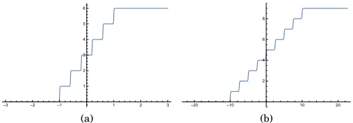
boundary value. where (SS) lies between -b and b. c is constant are chosen to formulate the shape of SS function in x and y axis. The (SS) function has the shape of smooth stair steps , where each step represents integer number of label ranking in y-axis from 0to ∞. as shown in Fig. 1, TheSS step is not absolute flat but it has differential slope, The function boundary onx-axis has range from -∞ to ∞ Therefore,NN input feature values are required to be normalized from -1 to 1 on the x-axis. The step width is 1 when n'2b. The convergence rate based on the step width. However it may take less time to converge based on NN hyper parameters. The Fig. ??(a) and (b) shows the activation functions to rank 6 and 9 labels respectively.
-3 -2 -1 1 2 3
1 2 3 4 5 6
(a)
-20 -10 10 20
2 4 6 8
(b)
Fig. 3: SS activation function where n=6 and boundary
b=1 in (a).n=9 and boundaryb=10 in (b)
B. Ranking high number of labels
By increasing number of labels, Data separability de-creases. We use Fishe LDA to measure the separability of the data. Scaling value for features and activation function is calculated using Eq.??
S=100·(1−λi) (3)
(i) Increase SS activation function boundaries by in-creasing b value of equation to make the step width not less than 1.
(ii) Increase the data separability of features by scaling the data up to the SS activation function boundaries. as shown in Fig ??. i.e, S=20, the SS Activation function boundaries and features scaling is -20 to 20. Algorithm 1 represents the classical three functions of the NNlearning process; feed forward, back-propagation, and updating weights.
Algorithm 1:PNN learning flow
Data:
D∈{〈x1,π1〉, {〈x2,π2〉, ....,〈xn,πn〉} (4)
Result:
L={λy1, ....,λy n} (5)
1 Randomly initialize weights ωi,j∈{−0.5, 0.5}
2 repeat
3 forall 〈xi,πi〉 ∈Ddo
4 ai|l−1=Pmi=1ϕ(ai·ωi)|n // Feedforward
5 Backpropagation()
6 ωi new =ωi old−η·δi //Update Weights
7 until τAv g = 1 or#iterations≥106;
Algorithm 2:PNN backpropagation
8 for l in L-1 to 1do
9 ifl=L-1then
10 for each i in layer ldo
11 ρ= −6·(2yti−yi)/m(m2−1) //Spearman error
12 else
13 for each i in layer ldo
14 Erri=ωi·δi
15 for each i in layer ldo
16 ∆·δi=Err·ϕ0
C. Ranking Loss Function
Two main error functions have been used for label rank-ing; Kendall τ [?] and Spearman [?]. However, Kendall error function lack continuity and differentiability. There-fore,PNNspearman correlation coefficient to measure the ranking between output labels.Spearmanerror derivative is used as a gradient ascent process only for backprop-agation and correlation is used as a ranking evaluation function for convergence stopping criteria. τAv g is the averageτper each label divided by number of instancesm, as shown in line 8 of Algorithm 1.PNNtype B uses Spear-man correlation coefficient function and it’s derivatives to calculate the gradient ascent and error stopping criteria. PNN by PSSor SSfunctions takes less calculation time
to reach ranking accuracy 100%, As shown in fig ?? in
result section where type A has low RMS comparing to
Spearman.
Spearman error function which is represents by the Eq.??
ρ=1−6
Pn
i=1(yi−yti) 2
n(n2−1) (6)
where yi, yti, i and m represent rank output value, expected rank value, label index and number of instances, respectively.
D. PNN Structure
1) Type A: has traditional neural network architecture. It is fully connected single-hidden layerNNand multiple-valued neuron has single activation function. The input layer represents the number of features per data instance. The hidden neurons are equal to or greater than the number of output neurons,Hn≥L, in order to reach error convergence after a finite number of iterations. The output layer represents the labels indexes as neurons, where the labels are displayed in fixed order as shown in Fig.??
2) Type B: Scaling type A is increasing the number of hidden neurons only because increasing hidden layer does not increase ranking because it doesn’t increase arbitrarily complex decision regions and degrees of freedom to solve
rank more complex problem. this limitation due to SS
activation function which doesn’t have variation in output values. Therefore, instead of increasing hidden layer , We propose duplication of output layers. this duplication equal to duplication of network from middle to output layer. All these duplicated networks share the weights between in-put and middle layer. This increasing in number of weights between middle and duplicated output layers increase the number of connection in the system thus increase degree of freedom. This increasing number of weights using the same number of hidden neurons. requires to duplicate activation functions. therefore hidden neuron serve more than one network.
Type B has different architecture to speed up the learning. We introduce hidden neuron multiple activation functions. The duplication of activation functions equal to the duplication of multi label group. each activation func-tion linked to one clone of output labels. as shown in fig
?? (b). Weights are duplicated between middle layer and output layer. This type of enforcement learning reduces the number of iterations and speed up the convergence rate as shown in Fig ??(b).
(a) (b)
Fig. 4: Sample output images of video file demonstrate the evaluation of PNN type A and B using SSfunction after 20 iterations in (a) and (b) respectively. [?]
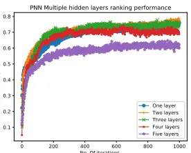
0 200 400 600 800 1000 No. Of iterations
0.1 0.2 0.3 0.4 0.5 0.6 0.7 0.8
Ta
u
PNN Multiple hidden layers ranking performance
One layer Two layers Three layers Four layers Five layers
Fig. 5:PNNType A SS ranking performance is decreasing by increasing the number of hidden layers
4) Multiple-Activation functions: In Type B each hidden neuron contain more than one activation function. the
activation function has the same type PSS or SS and
has equal number of labels n. middle neuron could have double, triple, or quadratic functions. each function is
connected to different output layer which represent a clone of the multi-labels. as shown in the architecture in Fig. ??.
Fig ?? represents type A and B for a small dataset
by reaching ranking correlation = 1 after a small finite
number of iterations. as shown in Fig ?? the output
labels represents the ranking values. The differential SS function helps to reach the convergence after few number of iterations due to Staircase shape which achieve the stability in learning.
In order to map sub-grouping to the label ranking,
PNN assigns the same ranking values to more than one
label. Thus,NN structure solves the problem of multiple subgroup ranking where number of ranking values is less the number of output labels, i.e., π=λdÂλbÂ(λc,λa), where λd=1,λb=2 and (λc'λa) = 3 as shown in Fig. ??.
PNN calculates preference values of the output labels
based on the boundedSSactivation function. Each neuron uses activation function in feedforward propagation to
calculate the preference number from 1 to n, where n
both SS and error function are differentiated as shown in Eqs. (10)-(13) and (14)-(15), respectively. The process of feedforward and backpropagation are iterated until the average of Kendall τ coefficient of all data is equal to one (τAv g=1) or the number of iterations reaches (106) as shown in Algorithm 1.
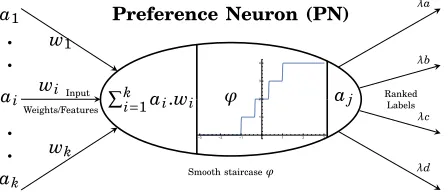
Preference Neuron (PN)
Smooth staircaseϕ
Ranked Labels Input
Weights/Features
a1 w1 . .
ai wi
. .
ak wk
λa
λb
λc
λd
aj
Pk
i=1ai.wi ϕ
-3 -2 -1 1 2 3 1 2 3 4
Fig. 6: Preference neuron single function whereϕn=4
where τ, Sgn,yi, yti, i, j and m are Kendall τ co-efficient, sign function, output ranking value, expected ranking value, label indexes and number of instances. Incomparable label are excluded from (??)
IV. PNNBACKPROPAGATION
A. Backpropagation of Output Layer
In this step, SS activation and the error function are differentiated for every hidden neuron as given in Eq. ??.
∂τ ∂ωL=
∂τ ∂yL·
∂yL
∂yaL·
∂yaL
∂ωL
(7)
where yaL is the neuron output before the activation
function for middle layer L. For type B, We have multiple output layers and multiple Activation functions as in Eq.
??
∂τ ∂ωLm =
∂τ ∂yLm·
∂yLm
∂yaL ·
∂yaL
∂ωLm
(8)
Where m is the number of activation functions.
The differentiation of the four labels ranking activation function is represented in Eqs. (??)-(??).
∂yL
∂yaL = − 1/2·
3 X
i=0
(1−tanh(−k·yaL·(k−(2·k·i/n−1))2) (9)
∂τ ∂wL=
∂τ ∂yL·
∂yaL
∂wL·− 1/2·
3 X
i=0
(1−tanh(−k·yaL·(k−(2·k·i/n−1))2)
(10)
∂τ ∂wL=
∂τ ∂yL·
HL·−1/2·
3 X
i=0
(1−tanh(−k·yaL·(k−(2·k·i/n−1))2)
(11) The differentiation of Spearman correlations objective function for output layer is given in Eq.??
∂ρ ∂yL=
12(yL−yLytL)
n(n2−1) (12)
ωLnew=ωLold−η·
∂ρ ∂wLold
(13)
whereη,ωLandaare the learning rate, weight ofH1and output node, respectively as shown in Fig. 4.
ωLnew=ωLold−η·
∂ρ ∂yL·
∂y1 ∂yaL·
HL (14)
B. Backpropagation of Middle Layer
This section shows the calculation of the weights of input neurons of hidden layer using Eqs.(??)-(??).
∂ρtotal
∂wL−1 = ∂τ ∂HL−1·
∂HL−1 ∂HaL−1·
∂HaL−1 ∂wL−1
(15)
where Ha is the hidden neuron output before the activa-tion funcactiva-tion.
∂ρtotal
∂wL−1 = ∂τL
∂HL·
∂HL−1 ∂Ha·L−1·
∂Ha·L−1 ∂ωL−1
(16)
∂ρL
∂HL=
∂ρL
∂yaL·
∂yaL
∂HL
(17)
ωL−1new=ωL−1old−η.∂ρtotal
∂ωL−1
(18)
ωL−1new=ωL−1old−η.
∂ρL
∂HL
· −1/2· 3 X
i=0
(1−tanh(−k·yaL·(k−(2·k·i/n−1))2) (19)
V. PROOF OF CONVERGENCE
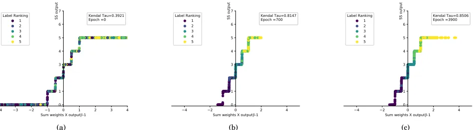
Ranking convergence is visualized by plotting the value for each output neurons before applying activation func-tion on x-axis and the output after activation function as shown in Fig. 5 - 7 where the point colors represents the actual ranking and y-axis represents the output ranking. By increasing the number of iterations, The ranking ac-curacy is increased. The τ rate changes according to the shape activation function with the same hyper parameters.
For example, SS has τ=0.8 in 80 epochs. However, PSS
takes 30 epochs as shown in in Fig ??. This τ variation
is due to the PSS curve smoothness between steps and
staircase location on both sides of y-axis. The comparison between SS and PSS by different edge smoothness is shown in Fig.??
The output of preference neuron ais obtained from the activation function ϕgiven in Eq.??
aj=ϕ(ωT·ai) (20) whereaiandajare neuron input and output, respectively. The neural output behavior is shown in Eq. ??
{a1,t1}, {a2,t2}, ..., {aj,tq} (21)
where each target outputtq is the preference value equal to 1, 2, 3,.., n.
The total inputs to the preference neuron is calculated as the following after neglecting the bias.
w1m w14
w13
w12
w11
w2m w 24 w23 w22 w 21
w3m w34
w33
w32
w31
w4m w44
w43
w
42
w41
wm4
wm3
wm2
wm1
w84
w83
w82
w81 w74
w73 w 72 w71 w64 w63 w62 w61
w54w53
w52
w51
Output
layer λd
Â
λb
Â
(λ
c,λ
a) 3 2 3 1 d c b a F4 F3 F2 F1 Instance / Object H 1 H 2 H 3 H 4 H 5 Middle layer ϕn =4 -3 -2 -1 1 2 3 1 2 3 4 Input layer (a) Output la yer 1 λ d  λb  λc  λa 4 2 3 1 Output la yer 2 λd  λb  λc  λa 4 2 3 1 Output la yer 3 λd  λb  λc  λa 4 2 3 1 d c b a d c b a d c b a F4 F3 F2 F1 Instance /Object H 1 H 2 H 3 H 4 H 5 Middle layer ϕ n =4 -3 -2 -1 1 2 3 1 2 3 4 Input layer (b)
Fig. 7: PNN type A and B architecture in (a) and (b) respectively whereϕn=4, fin=4 andλout=4.
TABLE I: PNN types.
Type A B
Arch. Full. Connected, FF-NN Partial Connected, FF-NN
Neuron Multi. Value, Single function
Output Layer Single Layer Multi. Layer
Activation Fun. PSS, SS
Gradient Ascent Correlation.
Learning Err. Fun. Spearman
Stopping criteria Spearman
The weighted vector is given by Eq. (??).
ωnew=ωold+Eerr·z (23)
where Eerr is the ranking error value from 0 to n. After k iterations for which the weight changes, the learning process is shown in Eq. (??).
ω(k)=ω(k−1)+z0(k−1) (24)
The solution weighted vector ωs ranks all the input Q correctly. z0(k−1) is the appropriate member of the set as
shown in Eq. (41)
z1,z2,z3, ...,zQ. (25)
To get preference value for 1, 2 and 3, then tq=1, 2 and 3 as given in Eqs. (??)-(??).
ωT
sz1>δ>0 (26) ωT
sz2>δ>1 (27) ωT
sz3>δ>2 (28)
The objective of the proof of convergence is to find the upper and lower boundaries on the length of the weighted vector. Afterkiterations, it can be represented as Eq. (??)
ω(k)=z0(0)+z0(1)+ · · · +z0(k−1) (29)
By taking the inner product of the solution weighted vector
ωswith the weight vector ofkiteration, we can obtain Eq. (??)
ωT
s ·x(k)=ωTs·z0(0)+ωTs ·z0(1)+ · · · +ωTs ·z0(k−1) (30) Eqs. (??)-(??) and (??) are substituted as in Eq.??
ωT
s.z0(i)>δ (31) Therefore,
ωT
s·ω(k)>kδ (32) From the Cauchy-Schwarz inequality [?]
(ωTs.ω(k))2≤∥ωs∥2∥ω(k)∥2 (33) where
−4 −3 −2 −1 0 1 2 3 4 Sum weights X utput|l-1
0 1 2 3 4 5 6 7
SS
u
tpu
t
Label Ranking 1 2 3 4 5
Kendal Tau=0.3921 Ep ch =0 Kendal Tau=0.3921 Ep ch =0
(a)
−4 −2 0 2 4
Sum weights X utput|l-1 0 1 2 3 4 5 6 7
SS
u
tpu
t
Label Ranking 1 2 3 4 5
Kendal Tau=0.8147 Ep ch =700 Kendal Tau=0.8147 Ep ch =700
(b)
−4 −2 0 2 4
Sum weights X output|l-1 0 1 2 3 4 5 6 7
SS
ou
tpu
t
Label Ra ki g 1 2 3 4 5
Ke dal Tau=0.8506 Epoch =3900 Ke dal Tau=0.8506 Epoch =3900
(c)
Fig. 8: Visualizing PNN type A convergence of 5 labels usingSSactivation function on stock data set in (a), (b) and (c) after 0, 700 and 3900 epochs respectively.
From Eq. (49) we can put the lower bound on the squared length at iteration k :
∥ω(k)∥2≥(ω T sω(k))2 ∥ωs∥2 >
(kδ)2 ∥ωs∥2
(35)
To find an upper bound for the length of weight vector, the change in the length at iterationkis given in Eq. (53)
∥ω(k)∥2=ωT(k).ω(k) (36) ∥ω(k)∥2=[ω(k−1)+z0(k−1)]T[ω(k−1)+z0(k−1)] (37) ∥ω(k)∥2=ωT(k
−1)ω(k−1)+2ωT(k
−1)z0(k−1)+z0T(k−1)z0(k−1) (38) Eq. (52) can be simplified as
∥ω(k)∥2≤∥ω(k−1)∥2+ ∥z0(k−1)∥2 (39) Eq. (53) can be repeated for ∥ω(k−1)∥2 ,∥ω(k−2)∥2, to obtain
∥ω(k)∥2≤∥z0(0)∥2+ ∥z0(1)∥2+...+ ∥z0(k−1)∥2 (40) If Π=max{∥z0(i)∥}, this upper bound can be simplified to Eq. (58).
∥ω(k)∥2≤KΠ (41) The weights only change to a finite number of times
because k has upper bound. Therefore, the NN learning
converges after a finite number of iterations.
VI. EXPERIMENTALRESULTS
A. Activation Functions Evaluation
PNNis tested on iris data set using four activation func-tions.SS,PSS,Relu,SegmoidandTanh. The experimented NNhas 1 hidden layer and 50 neurons in the hidden layer and learning rate of 0.05. Fig. ??shows the convergence after 500 iterations using four activation functions (SS, PSS, Sigmoid, Relu and Tanh ) respectively. We noticed that SS has a stable rate of ranking convergence compar-ing to Sigmoid, Tanh and Relu. This stability due to the stairstep width that help each point to reach the correct ranking in less number of epochs.
0 100 200 300 400 500
No. Of iteration −0.4
−0.2 0.0 0.2 0.4 0.6 0.8
Ta
u
Activiton function performance for Ranking
SS PSS Relu Sigmoid Tanh
Fig. 9: PNN Type A Ranking conversion using the SS,
PSS, Sigmoid, Relu and Tanh activation functions using the iris data set and 500 iterations and learning rate of 0.05 using one hidden layer and 50 hidden neurons.
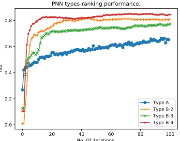
B. PNN types Evaluation
PNN Type A, B-2, B-3, B-4 are tested on iris Data set using hyper parameters(h.n.=50, L.r=0.07, epochs=100). as shown in Fig. ?? It can be noticed that Type B-4 reach high variance ranking accuracy training model comparing to type A.
C. Objective functions Evaluation
It can be noticed that Type A Spearman reach high variance ranking accuracy training model in 100 iterations
comparing type A. However, Type A RMS has lowerRMS
than Spearman as shown in Fig. ??
D. Data sets
PNN is experimented using three different types of
0 20 40 60 80 100 No. Of iterations
0.0 0.2 0.4 0.6 0.8
Ta
u
PNN types ranking performance,
Type A Type B-2 Type B-3 Type B-4
Fig. 10:PNNType A, B-2, B-3, B-4 performance evaluation on iris dataset
0 20 40 60 80 100
No. Of iterations 0.1
0.2 0.3 0.4 0.5 0.6 0.7
PNN Type A Objective function types performance ,Dropout= True
KendallType - RMS Kendall Tau SpearmanType - RMS Spearman Tau
Fig. 11: Objective functions RMS and Spearman inPNN type A ain iris dataset
where labels have repeated preference value [?]. German elections 2005, 2009 and modified sushi are considered new and restricted preference data sets. The second type is real-world data related to biological science [?]. The third type of data set is semi-synthetic (SS) taken from the KEBI Data Repository at the Philipps University of Marburg [?]. All data sets do not have ranking ground truth and all labels have a continuous permutation space of relations between labels. Table I summarizes the main characteristics of the data sets.
E. Results
PNN is evaluated by restricted and non-restricted label ranking data sets. The results are derived using spearman
ρ and converted to Kendall τ coefficient for comparison with other approaches. For data validation we use with ten-fold cross validation. to avoid over-fitting problem, Hyper-parameters i.e.(learning rate from 0.001 to 0.5, hid-den neuron from 25 to 200 neurons and scaling boundaries from 1 to 50) are chosen within each cross-validation fold by using the best learning rate on each fold and calculating
TABLE II: Three benchmark data sets for label ranking; preference mining [?], semi-synthetic (SS) [?] and real-world data sets
type data set category #inst. #attr. #lbl.
Mining data
algae chemical stat. 317 11 4
german.2005 user pref. 413 29 5
german.2009 user pref. 413 32 5
sushi user pref. 5000 10 10
top7movies user pref. 602 7 7
Real
data
cold biology 2,465 23 4
diau biology 2,465 24 6
dtt biology 2,465 24 4
heat biology 2,465 24 6
spo biology 2,465 24 11
Semi-Synthesized
data
authorship A 841 70 4
bodyfat B 252 7 7
calhousing B 20,640 6 5
cpu-small B 8192 3 4
elevators B 16,599 9 9
fried B 40,769 9 5
glass A 214 9 6
housing B 506 6 6
iris A 150 4 3
pendigits A 10,992 16 10
segment A 2310 3 4
stock B 950 5 5
vehicle A 846 18 4
vowel A 528 10 11
wine A 178 13 3
wisconsin B 194 16 16
TABLE III: Preference mining ranking performance in
terms of Kendall τ coefficient and learning step and
number of hidden neurons.
Preference mining exceptions Data
data set Avg.τ l.step #h.n.
algae 0.651 0.0001 100
german2005 0.89 0.0001 20
german2009 0.78 0.0001 20
sushi 0.69 0.0003 300
top7 movies 0.602 0.004 20
the average τ of ten folds. grid searching is using to get the best hyper parameter.
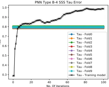
1) Preference Mining results: The ranking performance of the new preference mining data set is represented in table II. To enhance the ranking performance of the repeated label values of algae data set, a total 250 hidden neurons are used. However, restricted labels ranking data sets of the same type, i.e, (german elections and sushi) did not require high number of hidden neurons and took less computation cost.
0 20 40 60 80 100 No. Of iterations
0.3 0.4 0.5 0.6 0.7 0.8 0.9 1.0
Ta
u
PNN Type B-4 SSS Tau Error
Tau - Fold0 Tau - Fold1 Tau - Fold2 Tau - Fold3 Tau - Fold4 Tau - Fold5 Tau - Fold6 Tau - Fold7 Tau - Fold8 Tau - Fold9 Tau - Training model
Fig. 12:PNNtype B results iris evaluation and validation and using Dropout regulation and non-dropout in (a) and (b) respectively.
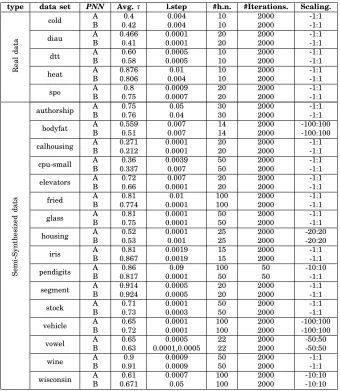
F. PNN Performance
During the experiment, it was found that ranking per-formance increases with an increase in the number of hidden neurons in hidden layers. All the results are held using single hidden layer with a various number of hidden
neurons from (50 to 300) and SS activation function.
Kendallτerror converges and reaches close to 1 after 2000 iterations as shown in fig 6.
Table IV compares PNN with the similar approaches
used for multi-label ranking. These approaches are; Deci-sion trees [?], MLP-LR[?] and label ranking trees forest LRT [?]. In this comparison, we choose the method that have promising results for each approach.
G. Missing Labels Evaluation
PNN is evaluated by removing a random number of
la-bels per each instance.PNNmarked the missing label as -1;PNNneglects error calculation during backpropagation,
δ = 0. Thus, the missing label weights remain constants per each learning iteration. Missing label approach is applied to the data set by 20% and 60% of the training data. It is noticed that ranking performance decreases when the number of the missing labels increases.However,
SS and PSS are more stable convergence than other
functions. This evaluation is performed on iris data set as shown in Fig. ??.
H. PNN Dropout Regularization
We apply dropout as a regularization approach to en-hance the neural network performance by reducing over-fitting. We dropout weights have probability with less than 0.5. The comparison between dropout and non-dropout of type A and B are shown in Fig. ?? ,??. the gap between training model and 10 fold cross validations curves has been reduced by using dropout of iris dataset.
0 100 200 300 400 500
No. Of ite ations −0.1
0.0 0.1 0.2 0.3 0.4 0.5 0.6
Ta
u
Activiton functions pe fo mance fo Ranking 60% labels missing
SS PSS Relu Sigmoid Tanh
Fig. 13: PNN type A Ranking conversion using the
Sig-moid, Tanh,Relu and SS activation functions using 60% missing labels iris data set and 500 iterations and learning rate of 0.05 using one hidden layer and 50 hidden neurons.
0 20 40 60 80 100
No. Of iterations 0.74
0.76 0.78 0.80 0.82
Ta
u
PNN Type A Tau Error Convergion ,Dropout= False
Tau - Fold0 Tau - Fold1 Tau - Fold2 Tau - Fold3 Tau - Fold4 Tau - Fold5 Tau - Fold6 Tau - Fold7 Tau - Fold8 Tau - Fold9 Tau - Training model
Fig. 14:PNNtype A results Iris evaluation and validation and using Dropout regulation and non-dropout in (a) and (b) respectively.
I. PSS and SS Evaluation
As shown in Fig ??, PSS for A and B reaches the
convergence in less number of iterations comparing toSS.
However, SS has lower RMS than PSS This is due to
two reasons: 1-SSsmoothness between staircase steps is almost 0, This hard smoothness make the results jump to integer ranking values, 2- The symmetry of SS function on x Axis. The SS shape handle both positive and negative normalized data. It reduces the number of iterations to reach the correct ranking values.
The biological real world data set was experimented using supervised clustering (SC) [?], Table V represents
the comparison between PNN Type A and supervised
clustering on biological real world data in terms ofLossLR as given in Eq. ??.
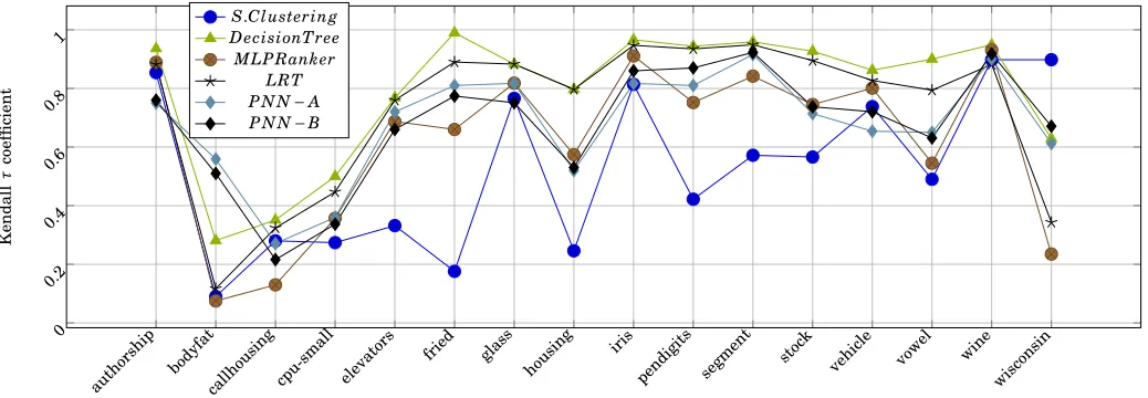
TABLE IV: PNN type A performance comparison with approaches: supervised clustering [?], supervised decision tree [?], multi-layer perceptron label ranking [?] and label ranking tree forest (LRT) [?]
Multi Label Ranking Methods
DS S.Clust. DT MLP-LR LRT PNN-A PNN-B
authorship 0.854 0.936(IBLR) 0.889(LA) 0.882 0.75 0.76
bodyfat 0.09 0.281(CC) 0.075(CA) 0.117 0.5591 0.51
calhousing 0.28 0.351(IBLR) 0.130(SSGA) 0.324 0.271 0.216
cpu-small 0.274 0.50(IBLR) 0.357(CA) 0.447 0.36 0.337
elevators 0.332 0.768(CC) 0.687(LA) 0.760 0.72 0.66
fried 0.176 0.99(CC) 0.660(CA) 0.890 0.81 0.774
glass 0.766 0.883(LRT) 0.818(LA) 0.883 0.8175 0.751
housing 0.246 0.797(LRT) 0.574(CA) 0.797 0.52 0.53
iris 0.814 0.966(IBLR) 0.911(LA) 0.947 0.817 0.867
pendigits 0.422 0.944(IBLR) 0.752(CA) 0.935 0.81 0.87
segment 0.572 0.959(IBLR) 0.842(CA) 0.949 0.916 0.923
stock 0.566 0.927(IBLR) 0.745(CA) 0.895 0.714 0.7374
vehicle 0.738 0.862(IBLR) 0.801(LA) 0.827 0.654 0.7204
vowel 0.49 0.90(IBLR) 0.545(CA) 0.794 0.65 0.631
wine 0.898 0.949(IBLR) 0.931(LA) 0.882 0.90 0.918
wisconsin 0.09 0.629(CC) 0.235(CA) 0.343 0.612 0.671
Average 0.475 0.79 0.621 0.730 0.6735 0.692
0 20 40 60 80 100
No. Of iterations 0.2
0.3 0.4 0.5 0.6 0.7 0.8
Ta
u
PNN Type A Tau Error Convergion ,Dropout= True
Tau - Fold0 Tau - Fold1 Tau - Fold2 Tau - Fold3 Tau - Fold4 Tau - Fold5 Tau - Fold6 Tau - Fold7 Tau - Fold8 Tau - Fold9 Tau - Training model
where τ is Kendall τ ranking error and LossLR is the
ranking loss function.
We use the SSS function with 16 steps to rank Wiscon-sin data set that has 16 labels. By increaWiscon-sing the number of steps in the interval and scaling up the features between -100 and 100, The step width is small. In order to enhance the ranking performance data set has many multi-labels, The number of hidden neurons is increased in order to exceed τ ranking 0.5 as shown in Fig.7.
Fig.9 compares the T au convergence rate between SS
and PSS activation functions using iris data set. The
learning step is 0.007 and number of iterations is 5000. We noticed theSSperforms better in fewer iterations than PSSusing the same hyper parameters. This is due to the pyramid shape where ranking values can be reached on both sides of y-axis. Thus, it minimize the iterations of back-propagation and weight updating to reach the correct ranking value.
J. Discussion and Future Work
It can be noticed from table III that PNN outperforms on SSdata sets withτAv g=0.825, whereas other methods
TABLE V: Comparison between PNN type A and
super-vised clustered on biological real world data in terms of LossLR
Biological real world data
DS S.Clustering PNN
cold 0.198 0.11
diau 0.304 0.255
dtt 0.124 0.01
heat 0.072 0.013
spo 0.118 0.014
Average 0.1632 0.0804
such as, supervised clustering, decision tree, MLP-ranker and LRT, have results τAv g= 0.79, 0.73, 0.62, 0.475, respectively. Also, the performance ofPNN is almost 50% better than supervised clustering in terms of ranking loss functionLossLR on biological real world data set as shown
in table V. PNN increases the number of iterations to
enhance the ranking performance of missing labels of iris data set as shown in Fig. 7.
The superiority of PNN for ranking is encoding the
multi-label preference relation to numeric values and rank
the output labels simultaneously. PNN could be used
to solve new preference mining problems. One of these problems is incomparability between labels, where Label ranking has incomparable relation ⊥, i.e., ranking space (λaÂλb⊥λc) is encoded to (1, 2, -1) and (λaÂλb)⊥(λcÂλd) is encoded to (1, 2, -1, -2).PNNcould be used to solve new problem of non-strict partial orders ranking, i.e., ranking space (λaÂλbºλc) is encoded to (1, 2, 3) or (1, 2, 2). Future research may focus on modifyingPNNarchitecture by adding bias and solving problems of extreme multi-label ranking.
VII. CONCLUSION
authorship bodyfat
callhousingcpu-small elevators
fried glass housing
iris
pendigits segment stoc
k
vehic le
vowel wine
wisconsin 0
0.2 0.4 0.6 0.8 1
K
endall
τ
coefficient
S.Clusterin g D ecisionT ree MLP Ranker
LRT P N N−A P N N−B
Fig. 15: Ranking performance comparison ofPNN with other approaches.
−4 −2 0 2 4
Sum weights X output|l-1 0.0
0.2 0.4 0.6 0.8 1.0 1.2 1.4
Sig
mo
id
ou
tpu
t
Label Ranking 0.00 0.25 0.50 0.75 1.00
Kendall Tau=0.3597 Epoch =200 Lrate =0.2
#h.n=30 Kendall Tau=0.3597 Epoch =200 Lrate =0.2 #h.n=30
(a)
−4 −2 0 2 4
Sum weights X utput|l-1 0.0
0.2 0.4 0.6 0.8 1.0 1.2 1.4
SS
u
tpu
t
Label Ranking 0.0 0.5 1.0 1.5 2.0
Kendall Tau=-0.0192 Ep ch =1100 Lrate =0.05
#h.n=50
Kendall Tau=-0.0192 Epoch =1100 Lrate =0.05 #h.n=50
(b)
Fig. 16: Ranking convergence of 5 labels usingSigmoidactivation function on iris data set in (a), (b) after 200, 1100 epochs respectively.
ranker NNuses SSto rank the multi-label per instance. The novelty of this neural network is overall error is mea-sured by ranking the preference value not by classification error for each neuron. Thus, it takes less computational time with single hidden layer. It indexing multi-labels as output neurons with preference values and proposing new activation function for ranking. The neuron output structure can be mapped to integer ranking value; thus,
PNN solves sub grouping ranking problems by assigning
the rank value to more than one output index. PNN is
implemented using python programming language and activation functions are modeled using wolframe software [?]. the videos of PNN types on small dataset is located [?]
ACKNOWLEDGEMENT
This work was supported in part by the Australian Re-search Council (ARC) under discovery grant DP180100670 and DP180100656.
REFERENCES
[1] J. Fürnkranz and E. Hüllermeier, “Preference Learning: An Intro-duction in Preference Learning”, Eds. Berlin, Heidelberg: Springer Berlin Heidelberg, 2011, pp. 1-17.
[2] R. Brafman and C. Domshlak. “Preference handling - an introductory tutorial”. AI Magazine, 30(1): 58-86, 2009.
[3] G. Adomavicius and A. Tuzhilin. “Toward the next generation of recommender systems: a survey of the state-of-the-art and possible extensions.” IEEE Transactions on Knowledge and Data Engineer-ing, 17(6):734-749, 2005.
TABLE VI:PNN ranking performance in terms of τcoefficient, learning step and number of hidden neurons. type data set PNN Avg.τ l.step #h.n. #Iterations. Scaling.
Real
data
cold A 0.4 0.004 10 2000 -1:1
B 0.42 0.004 10 2000 -1:1
diau A 0.466 0.0001 20 2000 -1:1
B 0.41 0.0001 20 2000 -1:1
dtt A 0.60 0.0005 10 2000 -1:1
B 0.58 0.0005 10 2000 -1:1
heat A 0.876 0.01 10 2000 -1:1
B 0.806 0.004 10 2000 -1:1
spo A 0.8 0.0009 20 2000 -1:1
B 0.75 0.0007 20 2000 -1:1
Semi-Synthesized
data
authorship A 0.75 0.05 30 2000 -1:1
B 0.76 0.04 30 2000 -1:1
bodyfat A 0.559 0.007 14 2000 -100:100
B 0.51 0.007 14 2000 -100:100
calhousing A 0.271 0.0001 20 2000 -1:1
B 0.212 0.0001 20 2000 -1:1
cpu-small A 0.36 0.0039 50 2000 -1:1
B 0.337 0.007 50 2000 -1:1
elevators A 0.72 0.007 20 2000 -1:1
B 0.66 0.0001 20 2000 -1:1
fried A 0.81 0.01 100 2000 -1:1
B 0.774 0.0001 100 2000 -1:1
glass A 0.81 0.0001 50 2000 -1:1
B 0.75 0.0001 50 2000 -1:1
housing A 0.52 0.0001 25 2000 -20:20
B 0.53 0.001 25 2000 -20:20
iris A 0.81 0.0019 15 2000 -1:1
B 0.867 0.0019 15 2000 -1:1
pendigits A 0.86 0.09 100 50 -10:10
B 0.817 0.0001 50 50 -1:1
segment A 0.914 0.0005 20 2000 -1:1
B 0.924 0.0005 20 2000 -1:1
stock A 0.71 0.0001 50 2000 -1:1
B 0.73 0.0003 50 2000 -1:1
vehicle A 0.65 0.0001 100 2000 -100:100
B 0.72 0.0001 100 2000 -100:100
vowel A 0.65 0.0005 22 2000 -50:50
B 0.63 0.0001,0.0005 22 2000 -50:50
wine A 0.9 0.0009 50 2000 -1:1
B 0.91 0.0009 50 2000 -1:1
wisconsin A 0.61 0.0007 100 2000 -10:10
B 0.671 0.05 100 2000 -10:10
0 200 400 600 800 1,000 0
0.1 0.2 0.3 0.4 0.5 0.6
number of iteration
K
endall
τ
coefficient
with scaling up without scaling up
Fig. 17: Performance of ranking wisconsine data set has 16 labels with and without scaling up approach.
[5] F. Aiolli,“A preference model for structured supervised learning tasks”, in Proceedings of the IEEE International Conference on Data Mining (ICDM) (2005), pp. 557-560
[6] K. Crammer and Y. Singer, “Pranking with ranking”, in Advances in
Neural Information Processing Systems (NIPS) (2002), pp. 641-647 [7] C. Burges et al., “Learning to rank using gradient descent,” presented
at the Proceedings of the 22nd international conference on Machine learning, Bonn, Germany, 2005.
[8] Y. Zhou, Y. Liu, J. Yang, X. He, and L. Liu, “A Taxonomy of Label Ranking Algorithms,” JCP, vol. 9, pp. 557-565, 2014.
[9] J. Furnkranz and E. Hüllermeier, “Pairwise Preference Learning and Ranking,” in Machine Learning: ECML 2003, Berlin, Heidelberg, 2003, pp. 145-156: Springer Berlin Heidelberg.
[10] J. Fürnkranz and E. Hüllermeier, “Preference Learning,” Springer-Verlag, 2010.
[11] S. Har-Peled, D. Roth, and D. Zimak, “Constraint classification for multiclass classification and ranking,” presented at the Proceedings of the 15th International Conference on Neural Information Process-ing Systems, 2002.
[12] P. L. H. Yu, W. M. Wan, and P. H. Lee, “Decision Tree Modeling for Ranking Data,” in Preference Learning, J. Furnkranz and E. Hüllermeier, Eds. Berlin, Heidelberg: Springer Berlin Heidelberg, 2011, pp. 83-106.
[13] C. R. de S ´a, C. Soares, A. M. Jorge, P. J. Azevedo, and J. P. da Costa, “Mining association rules for label ranking” in PAKDD (2), 2011, pp. 432-443.
[14] A. G. e. Ivakhnenko, V. G. v. Lapa, S. United, and S. Joint Pub-lications Research, Cybernetic predicting devices. New York: CCM Information Corp., 1965.
0 1 2 3 4 5 6 0
0.2 0.4 0.6 0.8 1
number of iterations 103
K
endall
τ
coefficient
PSS,b=5 PSS,b=100
SS
Fig. 18: Ranking comparison of wisconsin data set using
SS and PSS b = 5, 100 and SS respectively. Where b is
the step curve value Activation functions wherePSSwith sharp edges gives better performance.
the Method of Stochastic Approximation,” Soviet Automatic Control, Vol. 1, No. 3, 1968, pp. 43-55.
[17] R. Isermann, S. Ernst, and O. Nelles,“Identification with Dynamic Neural Networks - Architectures, Comparisons, Applications,” IFAC Proceedings Volumes, vol. 30, no. 11, pp. 947-972, 1997/07/01/ 1997. [18] J. Schmidhuber, “Deep learning in neural networks: An overview,”
Neural Networks, vol. 61, pp. 85-117, 2015/01/01/ 2015.
[19] X. Wang, T. Huang, and X. Liu, “Handwritten Character Recog-nition Based on BP Neural Network,” in 2009 Third International Conference on Genetic and Evolutionary Computing, 2009, pp. 520-524.
[20] G. Huang, H. Zhou, X. Ding, and R. Zhang, “Extreme Learning Machine for Regression and Multiclass Classification,” IEEE Trans-actions on Systems, Man, and Cybernetics, Part B (Cybernetics), vol. 42, no. 2, pp. 513-529, 2012.
[21] E. Hüllermeier, J. Furnkranz, W. Cheng, K. Brinker, “Label ranking by learning pairwise preferences”. Artif. Intell. 178, 1897-1916 2008. [22] O. Dekel, D.Manning, Y. Singer, “Log-linear models for label rank-ing”, in Advances in Neural Information Processing Systems, vol. 16 2003.
[23] Y. H. Jung and A. Tewari, “Online Boosting Algorithms for Multi-label Ranking,” ed. Ithaca: Cornell University Library, arXiv.org, 2018.
[24] C. R. de S ´a, W. Duivesteijn, P. Azevedo, A. M. Jorge, C. Soares, and A. Knobbe, “Discovering a taste for the unusual: exceptional models for preference mining,” Machine Learning, vol. 107, no. 11, pp. 1775-1807, 2018/11/01 2018.
[25] http://dx.doi.org/10.17632/3mv94c8jpc.2
[26] S. Har-Peled, D. Roth, D. Zimak, Constraint classification: A new approach to multiclass classification, in Proceedings of the Thirteenth International Conference on Algorithmic Learning, Theory 2002. [27] M. Grbovic, N. Djuric, S. Guo, and S. Vucetic, “Supervised clustering
of label ranking data using label preference information,” Machine Learning, vol. 93, no. 2, pp. 191-225, 2013/11/01 2013.
[28] W. Cheng et al., “Decision tree and instance-based learning for label ranking,” presented at the Proceedings of the 26th Annual International Conference on Machine Learning, Montreal, Quebec, Canada, 2009.
[29] G. Ribeiro, W. Duivesteijn, C. Soares, and A. Knobbe,“Multilayer perceptron for label ranking,” presented at the Proceedings of the 22nd international conference on Artificial Neural Networks and Machine Learning - Volume Part II, Lausanne, Switzerland, 2012. [30] W. Cheng and E. Hüllermeier, “Instance-based label ranking using
the mallows model,” in ECCBR Workshops, 2008, pp. 143-157. [31] M. Grbovic, N. Djuric, and S. Vucetic, “Learning from Pairwise
Preference Data using Gaussian Mixture Mosdel,” 2014.
[32] M. G. Kendall, “Rank Correlation Methods.” London, England: Griffin, 1970.
[33] C. Spearman, “The proof and measurement of association between two things,”The American Journal of Psychology, vol. 15, no. 1, pp. 72-101, 1904.
[34] A. Aiguzhinov, C. Soares, and A. P. Serra, “A Similarity-Based Adaptation of Naive Bayes for Label Ranking: Application to the Metalearning Problem of Algorithm Recommendation,”in Discovery Science, Berlin, Heidelberg, 2010, pp. 16-26: Springer Berlin Heidel-berg.
[35] C. R. de S ´a, C. Soares, A. Knobbe, and P. Cortez, “Label Ranking Forests,” Expert Systems, vol. 34, no. 1, 2017.
[36] Q. Song, H. Jin, X. Huang, and X. Hu, “Multi-Label Adversarial Perturbations,” ed. Ithaca: Cornell University Library, arXiv.org, 2019.
[37] Y. Yan, Y. Wang, G. Wen-Chao, Z. Bo-Wen, C. Yang, and Y. Xu-Cheng, “LSTM 2: Multi-Label Ranking for Document Classification,” (in English), Neural Processing Letters, vol. 47, no. 1, pp. 117-138, 2018 2018-03-03 2018.
[38] Y. Zhou and G. Qiu, “Random forest for label ranking,” (in English), Expert Systems with Applications, vol. 112, p. 99, 2018 Dec 01 2018-10-05 2018.
[39] B. Guo, C. Hou, J. Shan, and D. Yi, “Low Rank Multi-Label Classi-fication with Missing Labels,” in 2018 24th International Conference on Pattern Recognition (ICPR), 2018, pp. 417-422.
[40] V. Bergelson, “Part V: Theorems and Problems - 09. Ergodic Theo-rems.” Princeton: Princeton University Press, 2008, pp. 3-691. [41] Wolfram Research, Inc., Mathematica, Version 12.0, Champaign, IL
(2019).
[42] A. Elgharabawy. "PNN Convergence performance."
Video File, Feb. 26, 2020 [Video file]. Available:
https://drive.google.com/drive/folders/1yxuqYoQ3Kiuch-2sLeVe2ocMj12QVsRM?usp=sharing [Accessed: Jan. 28, 2020]. [43] G. Bologna, "Rule extraction from a multilayer perceptron with
staircase activation functions," in Proceedings of the IEEE-INNS-ENNS International Joint Conference on Neural Networks. IJCNN 2000. Neural Computing: New Challenges and Perspectives for the New Millennium, 2000, vol. 3, pp. 419-424 vol.3.