Volume 44, Number 3 (May 1991)

TABLE OF CONTENTS:

Vol. 44, No. 3, May 1991

ARTICLES

Measurement and Sampling

194

199

204

Correcting estimates of net primary production: Are we overestimating

plant production in rangelands?

by Mario E. Biondini, William K. Lauen-

roth, and Osvaldo E. Sala

Comparison of four methods of grassland productivity assessment based

on

Festucapallescens

phytomass data

by Guillermo E. Defosse and M.B.

Bertiller

Estimation of fecal output with an intra-ruminal continuous release

marker device

by Don C. Adams, Robert E. Short, Michael M. Bonnan,

and Michael D. MacNeil

PlantJAnimal Interaction

208

Grazing behavior and forage preference of sheep with

chronic locoweed toxicosis suggest IJO addiction

by M.H. Ralphs, K.E. Panter, and L.F.

James

Improvements

216 Influence ofseedbed microsite characteristics on grass seedling emergence

by Von K. Winkel, Bruce A. Roundy, and Jerry R. Cox

Effects of revegetation on suriicial soil salinity in panspot soils

by D.G.

Hopkins,

M.D. Sweeney, D.R. Kirby, and J.L. Richardson

Selecting

A

triplex canescens

for greater tolerance to competition

by Dar-

rell N. Ueckert and Joseph L. Petersen

Factors affecting weeping lovegrass seedling vigor on shinnery oak range

by William Matizha and Bill E. Dahl

215

220

223

Economics

227

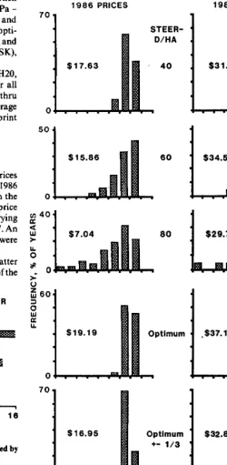
Managing range cattle for risk-the STEERISK spreadsheet

by Richard

H. Hart

232

Economics of broom snakeweed control on the Southern Plains

by Brent

D. Carpenter, Don E. Ethridge, and Ronald E. Sosebee

Plant Physiology

237

241

246

249

254

The effect of hormone, dehulling and seedhed treatments on germination and adventitious root formation in blue grama

by Rakhshan Roohi and

Donald A. Jameson

Defoliation effects on yield and bud and tiller numbers of two Sandhills

grasses

by J. Jeffrey Mullahey, Steven S. Waller, and Lowell E. Moser

Long-term effects of rangeland disking on white-tailed deer

browse

in

south

Texas

by Erasmo Montemayor, Tim E. Fulbright, Larry W. Broth-

ers, Bobby J. Schat, and Debra Cassels

Long-term tebuthiuron content of grasses and shrubs on semiarid range-

lands

by

T.N. Johnsen, Jr., and H.L. Morton

Published bimonthly-January, March, May, July, September, November Copyright 1991 by the Society for Range Management

lNDlVlDUALSUBSCRlPTlONisbymembershipin the Society for Range Management.

LIBRARY or other INSTITUTIONAL SUBSCRIP- TIONS on a calendar year basis are $56.00 for the United States postpaid and 568.00 for other coun- tries, postpaid. Payment from outside the United States should be remitted in US dollars by interna- tional money order or draft on a New York bank. BUSINESS CORRESPONDENCE, concerning sub- scriptions, advertising, reprints, back issues, and related matters, should be addressed to the Manag- ing Editor, 1639 York Street, Denver, Colorado 80206.

EDITORIALCORRESPONDENCE. concerning manu- scripts or other editorial matters, should be addressed to the Editor, Gary Frasier, 1300 Wheatridge Ct., Loveland, Colorado 80537. Page proofs should be returned to the Production Editor, 1839 York Street, Denver, Colorado 80206.

INSTRUCTIONS FOR AUTHORS appear on the inside back cover of most issues. A Style Manual is also available from the Society for Range Manage- ment at theaboveaddress@$2.00forsinglecopies; $1.25 each for 2 or more.

THE JOURNAL OF RANGE MANAGEMENT (ISSN 0022-409X) is published six times yearly for $56.00 per year by the Society for Range Management, 1839 York Street, Denver, Colorado 80208. SECOND CLASS POSTAGE paid at Denver, Colorado. POSTMASTER: Return entlre journal wlth address change-RETURN POSTAGE GUARANTEED-to Society for Range Management, 1839 York Street, Denver, Colorado 80206.

Managlng Edltor PETER V. JACKSON Ill

1839 York Street Denver, Colorado 80206 Editor

GARY FRASIER 1300 Wheatridge Ct. Loveland, Colorado 80537 Production Edltor PATRICIA G. SMITH

Society for Range Management 1639 York Street

Denver, Colorado 80206 (303) 355-7070

Grazing

259

Grazing systems, stocking rates, and cattle behavior in southeastern

Wyoming

by K.W. Hepworth, P.S. Test, R.H. Hart, J.W. Waggoner, Jr.,

and M.A. Smith

262

Cattle grazing behavior on a foothill elk winter range in southeastern

Wyoming

by R.H. Hart, K.W. Hepworth, M.A. Smith, and J.W. Wag-

goner, Jr.

267

Beef cattle distribution patterns on foothill range

by William E. Pinchak,

Michael A. Smith, Richard H. Hart, and James W. Waggoner, Jr.

Hydrology and Soils

276

Rangeland experiments to parameterize the water erosion prediction pro-

ject model: vegetation canopy cover effects

by J.R. Simanton, M.A.

Weltz, and H.D. Larsen

282

286

Use of stochastically generated weather records with rangeland simulation

models

by J.R. Wight and CL. Hanson

Effects of tree canopies on soil characteristics of annual rangeland

by

William E. Frost and Susan B. Edinger

General Interest

289

Research

Note: A survey of current range research activity

by Linda

H.

Hardesty

TECHNICAL NOTES

295

Evaluation of dietary preference with a multiple latin square design

by

Michael M. Borman, Don C. Adams, Bradford W. Knapp, and Marshall

R. Haferkamp

296

Monitoring roots of grazed rangeland vegetation with the root periscope/

mini-rhizotron technique

by Michael G. Karl and Paul S. Doescher

299

Germination of mechanically scarified neoteric switchgrass seed

by Nancy

K. Jensen and A. Boe

BOOK REVIEWS

302

Edwards Plateau Vegetation: Plant Ecological Studies in Central Texas.

Bonnie B. Amos and Frederick R. Gehlbach (eds.);

Wildlife Production

Systems: Economic Utilization of Wild Ungulates. 1989.

Edited by Robert

J. Hudson, K.R. Drew, and L.M. Baskin.

ASSOCIATE EDITORS DONALD BEDUNAH

School of Forestry University of Montana Missoula, Montana 59812 DAVID ENGLE

Agronomy Department Oklahoma State University Stillwater, Oklahoma 74078 TIMOTHY E. FULBRIGHT

College of Agriculture Texas A&I

POB 156, Sta. 1 Kingsville, Texas 78363 Book Revlew Edltor G. FRED GIFFORD DAVID L. SCARNECCHIA Range, Wildlife 81 Forestry

Department of Natural Resource Sciences loo0 Valley Road Washington State University University of Nevada Pullman, Washington 991648410 Reno, Nevada 89512

KRIS HAVSTAD USDA-ARS, Dept. 3JER Box 3003, NMSU

Las Cruces, New Mexico 88003 RODNEY HEITSCHMIDT

USDA ARS

Livestock & Range Research Rt 1 Box3

Miles City, Montana 59301 JERRY HOLECHEK

Animal 8 Range Science Dept. 3-l Box 30003 New Mexico State University Las Cruces, New Mexico 88003-0003 HERMAN S. MAYEUX, JR.

USDA-ARS

808 E. Blackland Road Temple, Texas 76502

KIRK MCDANIEL

Dept. of Animal 8 Range Science Box 31

New Mexico State University Las Crucea, New Mexico 88003-0003 ROY STRANG

British Columbia Inst. of Tech. 3700 Willingdon Ave. Burnaby, Brltlsh Columbia CANADA V5G 3H2 DAVID M. SWIFT

Natural Resources Ecology Colorado State Universlty Ft. Collins, Colorado 80623 PAUL TUELLER

President STAN TIXIER

2589 North 200 East Ogden, Utah 84414 1st VkcPresident JOHN L. ART2

2581 Westville Trail Cool, CA 95614 2nd Vke-President GARY DONART

Animal & Range Science New Mexico State University Las Cruces, New Mexico 88001 Executive Vke-President PETER V. JACKSON, Ill

Society for Range Management 1839 York Street

Denver, Colorado 80206 (303) 355-7070 Directors 19B9-1991

CHARLES E. JORDAN P.O. Box 1530

Rapid City, South Dakota 57709 PHILLIP L. SIMS

Southern Plains Range Research Station USDA, ARS

2ooO 16th Street Woodward, OK 73801 1990-1992

MURRAY L. ANDERSON 26 Clengarry Circle Sherwood Park, Alberta CANADA T8A 3A2 WILL H. BLACKBURN

NW Watershed Research NSDA-ARS

BOO Park Boulevard Plaza 4, Suite 105 Boise, ID 83712 1!391-1993

BARBARA H. ALLEN-DIAZ Department of Forestry and Resource Management

145 Mulford Hall, University of California Berkeley, California 94220

DEEN BOE

12714 Pinecrert Road Herndon, Virginia 22071

The term of office of all elected officers and direc- tors begins in February of each year during the Society’s annual meeting.

THE SOCIETY FOR RANGE MANAGEMENT,

founded in

1948 as the American Society of Range Management, is a nonprofit association incorporated under the laws of the State of Wyoming. It is recognized exempt from Federal income tax, as a scientific and educational organization, under the provisions of Section 501(c)(3) of the Internal Revenue Code, and also is classed as a public foundation as described in Section 509(a)(2) of the Code. The name of the Society was changed in 1971 by amendment of the Articles of Incorporation.

The objectives for which the corporation is established are:

-to properly take care of the basic rangeland resources of soil, plants and water;

-to develop an understanding of range ecosystems and of the principles applicable to the management of range resources:

-to assist all who work with range resources to keep abreast of newfindings and techniques in the science and art of range management;

-to improve the effectiveness of range management to obtain from range resources the products and values necessary for man’s welfare;

-to create a public appreciation of the economic and social benefits to be obtainedfrom the range environment;

-to promote professional development of its members.

Membership in the Society for Rang? Management is open to anyone engaged in or interested in any aspect of the study, management, or use of rangelands. Please contact the Executive Vice-President for details.

The Journal of Range Management

serves as a forum for the presentation and discussion of facts, ideas, and philosophies pertaining to the study, management, and use of rangelands and their several resources. Accordingly, all material published herein is signed and reflects the individual views of the authors and is not necessarily an official position of the Society. Manuscripts from any source-nonmenibers as well as members-are welcome and will be given every consideration by the editors. Editorial comment by an individual is also welcome and, subject to acceptance by the editor, will be published as a “Viewpoint.”

Correcting estimates of net primary production: Are we

overestimating plant production in rangelands?

MARIO E. BIONDINI, WILLIAM K. LAUENROTH, AND OSVALDO E. SALA

Abstract

This paper addresses the issue of the effect of random errors in field estimates of net primary production (NPP). This is a critical subject in range management because field estimates of plant pro- duction are regularly used to determine stocking rates, range con- dition, and animal consumption. What we show in this paper is that random errors associated with field estimates of NPP can result in a positive bias and thus an overestimation of NPP. Depending on the case, this overestimation has been reported as high as 700%. We present examples with overestimations in the 200% to 400% range. The overestimation in NPP increases with increases in biomass variances, frequency of sampling, and number of taxonomic (species) and tissue (live, dead, etc) components sampled. We (1) outline in nonmathematical terms the reasons behind overestimation in NPP and the analytical solutions designed to correct them; and (2) present applications of the analytical solution for adjustments to concrete cases. The adjustments for overestimation outlined in this paper do not guarantee an accurate estimate of NPP but eliminate an unneeded source of error. A computer program (for IBMTM compatible) designed to implement the necessary adjustments is available from the authors free of charge (send a blank diskette).

An article published by Singh et al. (1984) initiated a controversy in plant ecology about the accuracy of field estimates of net prim- ary production (NPP) based upon a time series of biomass. This controversy is of particular relevance to range science because field estimates of plant production are regularly used to determine range condition, stocking rates, and animal consumption. Accurate estimates of primary production are also very important for scien- tists and natural resource managers concerned with a wide variety of issues such as global carbon (C) budgets (Schneider 1989), soil organic matter, and herbivory.

Singh et al. (1984) used simulation models to show that most of the techniques used to estimate NPP (for a review see Singh et al. 1975) can overestimate net root production by as much as 70%. Similar results were reported for aboveground production by Lauenroth et al. (1986a). Both results contradicted previous assumptions that field estimates of NPP always underestimate NPP because biomass peaks may be missed and because of the simultaneous nature of production and decomposition. Singh et al. (1984) related NPP overestimation to the random errors associated with biomass estimates. They suggested that random errors can generate artificial peaks and troughs (false maxima and minima) in a time of series of biomass estimates which may lead to large overestimation of NPP. Vogt et al. (1986), however, challenged the conclusions of Singh et al. (1984) both on methodological grounds and by suggesting that they may be related to the peculiarity of the grasslands under study and thus not generally applicable. Subse- quently, Lauenroth et al. (1986b) answered the methodological

Authors are associate professor, Department of Animal and Range Sciences, North Dakota State University, Fargo 58105; professor, Department of Range Science, Colorado State University, Fort Collins 80523; associate professor, Departamento de Ecologia, Facultad the Agronomia, Universidad de Buenos Aires, Av. San Martin 4453, Argentina.

Support for this study was provided by the shortgrass steppe Long-Term Ecological Research program (NSF grant BSR-8 I 14822), the North Dakota Experiment Station and Consejo National the Investigaciones Cientificas y Tecnicas of Argentina (INT 151/87, PID 427/89). This is a North Dakota Experiment Station Publication Number 1898.

Manuscript accepted 23 July 1990.

194

questions raised by Vogt et al. (1986) but left open the problem of generating a statistical theory to explain why NPP overestimation may occur, and developing the analytical tools needed to correct them. Sala et al. (1988) provided the answer for both.

The objectives of this paper are: (I) to outline in nonmathematical terms the reasons behind overestimation in NPP and the analytical solution designed to correct it; and (2) present applications of the analytical solution for adjustments developed by Sala et al. (1988) to specific cases.

Random Errors and NPP Overestimation

We will use an example to explain the connection between random errors and overestimation of NPP (Fig. 1). Let’s assume that the mean biomass of a pasture is 110 g.me2 at time I (Bl) and 120 g.me2 at time 2 (B2), and furthermore, let’s assume that both means are normally distributed (Fig. la and 1 b). That implies that in the time 1 - time 2 interval there has been a mean increase in biomass (B2-Bl) of 10 g.mw2 which we would consider as the NPP for the period. Under field conditions, of course, we do not know the actual mean and standard deviation (sd) of the biomass in the pasture in question so we estimate it by sampling. For instance, 30 random samples from Figure la and 1 b, respectively, resulted in estimated meanand sd of 109.8 g.me2, 8.1 for Bl and I I8 g.mv2, 18.8 for B2. A t-test for a case of unequal variance (Snedecor and Cochran 1967) gives a t = 2.24 with a p q 0.028 (df = 39.5) confirm-

ing that there is in fact an increase in mean biomass in that period. Now, the underlying distribution of B2-Bl, which represents the differences in biomass between time 1 and time 2, is also normally distributed with a mean of IO g.me2and sd of 22.4 (Fig. lc). Sala et al. (1988) showed, however, that the underlying distribution of NPP estimates from all commonly used techniques is not normally distributed, but rather a combination of 2 distributions: a discrete distribution with mass at 0 and a truncated normal distribution (Fig. Id, and Appendix). The explanation can be intuitively cap- tured by the following argument. Even though the mean of B2-Bl is positive, there is a probability (0.33 in this example) that when sampling from Figure lc one would get a negative value by chance alone. NPP is not the difference B2-B I, but only the positive values of this difference. As a result, every time a negative value for B2-B I is obtained, NPP is assigned a value of 0. That represents the discrete portion of the NPP distribution that has mass at 0 (Fig. Id). When the difference B2-Bl is positive, we assign NPP that value, but the distribution of positive values is a truncated normal distribution rather than a normal one. Although the mean B2-Bl (actual NPP) is 10.g.me2, the mean derived from the distribution of

NPP estimates (we call it the calculated NPP) is 14.6 g.mm2. The difference between the actual and calculated values represents the overestimation observed by Singh et al. (1984).

Sala et al. (1988) developed equations that relate the calculated

NPP to the actual NPP, estimated the size of the overestimation, and developed algorithms needed to adjust the calculated NPP values to correct for overestimation (Appendix). Sala et al. (1988) also developed the theoretical proofs for results observed by Singh

et al. (1984): (1) overestimation increases as the variance of the estimated biomass increases; (2) the closer (though still signifi- cantly different) the mean biomasses are between 2 sampling peri-

DISTRIBUTION OF BIOMASS ESTIMATION ERRORS ASSOCIATED WITH SAMPLES TAKEN AT TIME 1

SD=10

I

ERROR DlSTRlBLlTiON FOR BIOMASS AT TIME 2 - BIOMASS AT TIME 1

C

I

I I I I 1 I

-20 -10 0 10 20 30 40

DISTRIBUTION OF BIOMASS ESTIMATION ERRORS ASSOCIATED WlTH SAMPLES TAKEN ATTIME 2

60 100 120 140 160

TRUE DISTRIBLVION OF NPP ESTIMATES

SD = 16.3

D

I I I I

0 10 20 30 40

Fig. 1. (a) and (b) represent the distribution of biomass estimation errors associated with samples taken at time 1 and time 2; (c) distribution of difference of biomass between time 2 and time 1; (d) actual distribution of NPP esthnates. For details see Appendix.

ods the higher the overestimation (as a percentage); and (3) increas- ing the frequency of sampling results in increasingly greater overestimation.

Example 1

In the following example we reanalyzed a subset of the Singh et al. (1984) NPP estimates of root biomass to show how the adjust- ment method is implemented and to compare the adjusted results with the published data. The data consist of the total root biomass (live + dead) generated by a simulation model for a 4-year period. Samples for a given date were generated by assuming that root biomass per sample period was normally distributed with mean equal to model estimates and a coefficient of variation of 0.32 (derived from Lauenroth and Whitman 1977). Ten samples were taken at 15-day intervals from 15 May through 1 September, and at 3O-day intervals from 1 September and through 1 November (Table 1). NPP was estimated as the sum of the significantly different (p<O.OS) increments in root biomass. The actual NPP (566 g.me2) in this case is a known value because it was generated from a simulation model.

According to theory (Singh et al. 1975), the use of a time series of total root biomass with statistical constraints should lead to a

substantial underestimation of root NPP because of missed bio- mass peaks, small biomass increments in relationship to standing crop, rapid biomass turnover, and translocation of C between shoots and roots (Wiegert and Evans 1964). Estimates of root production from harvest data, however, often result in overestima- tion. Results from the analysis of the Singh et al. (1984) data show that root NPP is overestimated by an average of 150% (Table 1). When we apply the adjustments developed by Sala et al. (1988), the estimates of NPP behave as expected by theory, that is they under- estimate actual NPP by an average of 33%. This is the desired behavior because underestimation in this case results from the limitations of the sampling method used rather than from a statis- tical artifact (the overestimation case) and can be reduced, if adjustments for overestimation are used, by more refined and intensive sampling protocols such as separating live and dead biomass, estimating decomposition and herbivory, and increasing the number and frequency of samples.

We use the case of Year 1 in Table 1 to illustrate how the adjustments are implemented. The procedure is as follows:

Step 1. Select a method to estimate NPP. In this example NPP is estimated as the summation of the significant (p<O.O5) incre- ments in total root biomass (live + dead) (Singh et al. 1984). As a consequence, adjustments will be calculated only in the cases where

Table 1. Reanalysis of the Singh et al (1984) NPP estimates of root biomass. The data for each sampling date represent mean and standard deviations for

total (live + dead) root biomass in g mm2 . Samples for a given date were generated by assuming that root biomass was normally distributed with mean equal to the model estimates and a coefflclent of variation of 0.32. Ten samples were taken per date. Four years are simulated. Root NPP was estimated as the summation of the significant (pC0.M) increments in root biomass (Sfngh et al. 1975). The actual value of root NPP (calculated from model flows) was 566 g m-* ye&.

May 15 June 1 June 1.5 July 1 July 15 Aug. 1 Aug. 15 Sep. 1 Oct. 1 Nov. 1 Actual NPP Estimated NPP Adjusted NPP Four Year Average

Total Root Biomass (g m-r)

Year 1 Year 2 Year 3 Year 4

Mean Sd Mean Sd Mean Sd Mean Sd

3080 492 3180 875 2665 179 3330 996

3197 875 3298 868 3120 1074 3181 879

2944 419 2800 1003 2644 808 3049 587

3468 909 3216 809 2812 700 2633 785

3210 894 :g 1272 3348 129 3417 834

2777 749 978 2929 1083 2895 1158

:% 361 3404 997 3165 882 3391 859

980 3563 889 3495 1385 3535 I133

3134 1154 2835 812 2741 1093 3252 1221

3339 706 3787 838 3748 983 3406 814

566 566 566 566

663 952 1007 784

353 528 360 278

Actual NPP 566

Estimated NPP 851

Adjusted NPP 380

there are significant increases in total root biomass between con- secutive dates.

Step 2. Identify all the significant (p<O.O5) increases in biomass between 2 consecutive dates. In this example the only significant increase takes place between 1 August and 15 August (3440 - 2777 = 663 g.m-‘). This represents the nonadjusted value.

Step 3. For all the cases where there is a significant increase in biomass, calculate the probability of finding by chance alone a decrease in biomass between the given dates (the area in the left hand side of Fig. lc). To do that, we first calculate the normal deviate z = -D/ SD where D is the difference in biomass between the 2 consecutive dates in question (B2-Bl) and SD = standard devia- tion of B2-B 1 = (Variance of B I+ Variance of B2)‘“. In our case D = 3440-2777~663, SD=[(749)2+(361)2]” q 831 andz=-663/831 q

-0.8. Second, calculate the value q = P (Z<-O.8) using a table for the cumulative standard normal distribution. To do that we first look at the table value for z = 0.8, using for instance Table A3 (page 548) of Snedecor and Cochran (1967), and then calculate q = 0.5 - z. In this case z q 0.2881 and q q 0.5 - 0.2881 = 0.21.

Step 4. To eliminate the effect of overestimation, i.e., calculate the adjusted mean and standard deviations, we need to solve equations (1) and (2), shown in the Appendix, where E(NPP) = B2 - Bl, Var (NPP) = (SD)2 and p = 1-q. In our particular example E(NPP) = 663, Var (NPP) = (831)2= 691,322, p = l-0.21 ~0.79. The values we need to solve for are p, which represents the adjusted (for overestimation) mean difference in total biomass between 1 August and 15 August and u, which represents the corresponding adjusted standard deviation. Replacing E(NPP), Var(NPP) and p in equations (1) and (2) of the Appendix with the values shown above led to the following system of equations to be solved:

663 = 0.79~ + a(0.4)(2.72)0.5~/“)2

691,322 = 0.79/.$(0.21) + 0.79~2 + ~~r(0.4)(2.72)“~~(~+‘)~(-0.58) - a2(0. 16)(2.72)+‘“2

The equations are solved for p and u using an approximation algorithm developed by Sala et al. (1988). The process is iterative in nature and stops when the right and left side of the equations differ by less than 5%. In this case p = 353 and u = 1055 are the solutions. A computer program has been developed by the authors for this

196

purpose and is available free of charge. The program tests for significant differences between means and solves for p and u. The only inputs required are mean biomass, standard deviation, and number of observations for each time period.

Step 5. Once all the significant biomass differences between consecutive dates are adjusted, NPP is calculated according to the selected method. In this case there was only 1 significant increment in biomass between consecutive dates therefore adjusted NPP q p =

353 rather than 663 g.

Once adjustments for overestimation are performed, more sophisticated methods for field estimations of NPP that involve frequent sampling, separation of live and dead material, estimation of decomposition rates, and estimations of C translocation (Sala et al. 1981) can be safely used to obtain more accurate estimates of NPP without the risk of incurring the large overestimation shown by Singh et (1984).

Example 2

In this example, we show the estimation of aboveground NPP with a method that accounts for changes in live biomass of individ- ual species, standing dead biomass and litter. The data for the example comes from Sala et al. (1981). NPP is calculated in 2 ways: (1) using a time series of live biomass only; and (2) using a time series of live biomass plus changes in standing dead and litter to account for senescence and decay processes.

Method 1 involves the summation of significant (pCO.05) increments in live biomass between consecutive dates for all species (Table 2). For example, Bothriochloa laguroides has significant increases in biomass in the December (1974) to January (1975), January to April and October to December (1975) intervals. The non adjusted biomass increments are 7.5, 6.7, and 13.2 g.me2, respectively. To adjust, we follow the same 4 steps of example 1 and apply it to each pair of consecutive dates. The adjusted biomass increments are 5.8,O (the actual value is -2.7 but the protocols for this method involve only biomas increments) and 3 g.mm2. The same procedure is repeated for each species, and the nonadjusted and adjusted for (overestimation) NPP estimates are calculated by summing all the increments (Table 2).

Method 2 involves corrections to the NPP values of Method 1 by

Table 2. Reanalysis of Sala et al. (1981) NPP estimates. Data is given in &mm*. NPP is calculated 2 ways: (1) sum of significant (pCO.05) @tive increments of live biomasq (2) as In 1 plus correction factors for senescence and decay processes using a time series of standing dad and Utter. Senescence corrections were caicul&d as the increments in standing dud not juslified by the summation of decreases in the live biomass of individual species. The decay correction factor was calculated as the increases in litter not jostifled by decreases in standing crop. For details on the calculations see text and Sale et al. (1981).

Species

December 1974 January April August October December 1975

Bio- Bio- Bio- Bio- Bio- Bio-

mass Sd n mass Sd n mass Sd n mass Sd n mass Sd n mass Sd n

Bothriochloa kaguroides Briza subaristata Danthonia

montevidensis Distichlis sp. Lolium multiflorum hfelica brasiliana Paspalum dilatatum Paspalum vaginatum Sporobulus indicus Sporobulus platensis Stipa neesiana Carexphalaroides Stipa papposa Ambrosia tenuifolia Juncus imbricatus Heleocharis sp. Stenotaphrum

secundatum Panic-urn millioides Panicum gouinii Panicum bergii Piptochaetium

montevidense Aristida murina Stipa bavioensis Setaria geniculata Agrostis hygrometrica Bromus unioloides Alophia amoena Lillaea sp. Eragrostis lugens

Forbs Other grasses Standing dead Litter

38.9 34.1 33 1.8

32.7 27.4 40 24.4 20.0 33

1.6 33 9.3

16.2 11.0 40 6.8 40

15.7 14.9 33 27.5 20.4 40 16.7 20.0 33 0.1 0.9 40 3.7 13.6 33 2.0 5.5 40 0 0 33 2.4 12.3 40 1.5 1.7 33 1.2 1.9 40 1.9 3.9 33 2.9 2.4 40 4.6 9.9 33 19.2 32.7 40 31.0 25.4 33 17.4 16.8 40 16.8 18.3 33 15.3 15.0 40 21.4 10.4 33 30.1 18.4 40 0 0 33 8.3 6.4 40 0.2 0.8 33 0 0 40

0 0 33 0 0 40

0 0 33 0 0 40

0 0 33 0 0 40 0.7 1.640 0 040 0 040

0 0 33 0 0 40 0.3 1.440 0 040 0 040

0 0 33 0.4 1.2 40 I.5 7.2 40 0 0 40 0 0 40

0 0 33 0 0 40 0.1 0.6 40 0 0 40 0 0 40

0 0 33 0 0 40 0.3 1.7 40 0 040 0 040

0 0 33 0 0 40 0.2 0.4 40 0 0 40 0 0 40

0 0 33 0 0 40 0.1 0.1 40 0 040 0 040

0 0 33 0 0 40 0 0 40 0.1 0.2 40 0 0 40

0 0 33 0 0 40 0 0 40 0.1 0.4 40 0 0 40

0 0 33 0 0 40 0 0 40 0.1 0.2 40 0.2 0.1 40

0 0 33 0 0 40 0 0 40 0.7 0.7 40 0.1 0.1 40

0 0 33 0 0 40 0 040 0 0 40 0.1 0.2 40

18.3 12.3 33 7.8 6.4 40 7.0 5.9 40 4.0 5.2 40 0.8 0.9 40 1.9 2.1 33 4.0 3.3 40 6.4 9.5 40 I.5 1.7 40 1.2 1.6 40 276.8 128.5 33 398.6 Ill.9 40 387.1 152.4 40 430.8 132.8 40 443.9 124.4 40 137.6 54.4 33 137.6 54.4 40 125.6 65.8 40 81.3 50.7 40 129.9 53.3 40 NPP with method 1

Adjusted NPP with method 1 NPP with method 2 Adjusted NPP with

method 2

188.1 47.7 430.2 195.7

16.0 15.5 40 2.4 2.3 40 1.2 1.0 40 18.3 17.7 40 39.2 24.4 40 65.5 39.5 40 21.8 15.5 40 26.3 14.3 40 48.9 23.1 40

19.1 4.4 40 6.9 4.7 40 5.8 4.5 40 0 0 40 1.2 2.3 40 0.1 0.1 40 0.5 2.4 40 1.3 3.3 40 I.0 3.8 40 6.5 40.3 40 0.7 3.1 40 0.7 2.4 40 :::

1.6 40 0.1 0.3 40 0.2 0.2 40 3.0 40 2.5 2.0 40 2.2 1.8 40 11.0 24.1 40 13.7 25.9 40 8.5 25.7 40 18.0 113.0 40 19.4 151.3 40 22.5 21.2 40 12.7 107.9 40 20.4 24.7 40 34.2 36.4 40 24.4 15.5 40 16.2 7.7 40 13.2 8.0 40 14.6 12.1 40 2.2 I.5 40 1.2 1.3 40

0.1 0.4 40 0 040 0 040

0.1 0.4 40 0 0 40 0 0 40

0.5 2.0 40 0 0 40 0 0 40

14.4 21.2 45 51.2 29.8 45 33.5 15.9 45 16.0 15.7 45 0 0 45 1.8 7.2 45 0.8 3.4 45 I.5 2.6 45 2.8 2.8 45 12.6 29.9 45 33.0 23.5 45 21.9 25.8 45 17.4 9.2 45 5.3 5.6 45 0 0 45 0 0 45 0 0 45 0 0 45 0 0 45 0 0 45 I.4 6.3 45 0.1 019 45 0 0 45 0 0 45 0 0 45 0 0 45 0 0 45 0 0 45 0 0 45 3.7 3.7 45 5.4 4.7 45 628.8 173.1 45 128.5 53.6 45

taking into account senescence and decay (Sala et al. 1981). The senescence correction is calculated as the increases in standing dead that are not justified by the sum of the decreases in the live biomass of individual species. For example, if between time 1 and time 2 a set of species shows a decrease in live biomass of 10 g.m-‘, but the increase for the same period in standing dead biomass is 15 g. rne2, the difference of 5 g.mm2 represents the senescence adjust- ment which is added to the estimates of Method 1. The decay correction involves decreases in standing dead biomass that are not justified by increase in litter. For example, if between 2 sample periods the increases in litter are higher than the decreases in standing dead biomass, the difference represents a decay adjust- ment and is added to the estimates of Method 1. For the rationale behind these adjustments see Sala et al. (1981).

Adjustments for increases in standing dead and litter are accomplished with the use of the same 4 steps of example 1. Decreases in live and standing dead biomass between 2 sample periods can be treated as increases by changing the time direction

(Bl-B2 rather than B2-Bl, which is equivalent to calculating the Abs(BZ-B 1)) and adjusted by following the same 4 steps of example 1. For example, let’s look at the case of forbs in the December 1974 to January 1975 interval: (a) we first check that the decrease in live biomass of -10.5 g.mm2 is in fact statistically significant (which it is at p<O.O5); and (b) as in step 3 of example 1 we calculate the adjustment by solving the system of equations (1) and (2) of the Appendix. In this case E(NPP) q Abs(-10.5) = 10.5, Var (NPP) q (12.3)2 + (6.4)2 q 192.25, z = -10.5/(192.25)‘” = -0.76, p = 1 - P(Z<-O.76) = 0.22. The adjusted decrease of biomass was 5.1 g.me2.

Danthonia montevidensis, Lalium multiflorum. Stipa neesiana also had significant decreases in live biomass for the period, which amounts to 8.2, 16.6, and 13.6 g.me2 respectively. The correspond- ing adjusted values are 0 (the actual adjusted value is -5.6, thus the 0), 9.5 and 0 (actual value -4.5). For the same period, there is a significant increase in standing dead of 121.8 g.mm2 (49.9 g.mm2 adjusted) which is greater (p<O.O5) than the sum of the decreases (adjusted and nonadjusted) in live biomass of individual species.

The senescence correction factor is then equal to a nonadjusted 72.9 g.m-’ (121.8-8.2-16.6-13.6-10.5) and adjusted 35.3 g.m-’ (49.9-9.5-5.1). The decay correction is calculated in a similar manner using decreases in standing dead and increases in litter. This procedure is repeated for every consecutive date that shows significant differences in standing dead and litter. NPP is then calculated by adding the correction factors to the NPP estimates of Method 1 (Table 2).

Discussion and Conclusions

The main methodological difference between the 2 examples shown in this paper is number of taxonomic (species) and tissue categories (live biomass, standing dead, and litter) used. We used only 1 category (total root biomass) in example 1, while in example 2 we used 33 (live biomass of 31 species plus standing dead and litter). The differences found between nonadjusted and adjusted (for overestimation) estimates of NPP in example 2 were 394% for method 1 and 455%for method 2, which are far higher than the one found in example 1 (200%). This differences can be explained by another of Sala et al. (1988) results that showed that increasing the number of sampling components is equivalent to increasing the frequency of sampling, both of which lead to increases in NPP overestimation if values are not properly adjusted. If adjustments are performed, however, increasing the number of plant categories sampled, the frequency of sampling, or both, increases the accu- racy of the NPP estimates by reducing the biomass peaks that are missed, and by accounting for senescence. We want to emphasize, however, that overestimation is not the only factor that can affect estimates of NPP based on harvest techniques. The main source of error is still the difference between the concept of NPP and the way we calculate it. In a strict sense NPP is the difference between the energy fixed by autotrophs and their respiration. All the tech- niques we commonly use to estimate NPP are an approximation to that value and thus, as we explained before, tend to lead to under- estimation. The peculiarity of the overestimation problem, how- ever, is that it is strictly the result of a statistical artifact related to the empirical way we estimate NPP and thus can be rigorously dealt with by the use of an appropriate statistical method. Adjust- ments for overestimation do not guarantee an accurate estimate of NPP but eliminate an unneeded source of error.

The general conclusions that can be made on the subject of overestimation are as follow:

1. Random errors associated with field estimates of above- or belowground biomass do not cancel each other but always result in a positive bias which may result in overestimation of NPP.

2. The overestimation in NPP increases (as a percentage) with (a) increases in the variance of biomass estimates, (b) decreases in the difference (though still statistically significant) in mean bio- mass between time periods, and (c) increases in the frequency of sampling and/or the number of tissue categories and taxonomic groups sampled. This overestimation can be as high as 700%. We presented examples with overestimation in the 200% to 400% range for above- and belowground NPP.

3. Sala et al. (1988) developed the statistical theory for the overestimation problem and the analytical solution to deal with it. The authors have developed a computer&rogram to implement it. The program can be run on any IBM compatible PC and is available from the authors free of charge (send a blank diskette).

4. Once adjustments for overestimation are performed, more sophisticated methods for field estimations of NPP that involve frequent sampling, separation of live and dead material, estimation

of decomposition rates, and estimation of C translocation (Sala et al. 1981) can be safely used to obtain more accurate estimates of NPP without incurring overestimation.

5. Adjustments for overestimation in NPP are critical in range management because of the central role that estimates of plant production have in determinations such as range condition and stocking rates, the design of grazing systems, and the estimation of animal consumption.

APPENDIX

In this section we present statistical relationships between actual

and field estimations of NPP developed by Sala et al (1988).

1. Distribution function of NPP estimates

FNPPWP) = q + GcNPP(NPP) (Cumulative Distribution) where GcurP(NPP) = (27r)-1’(op)-1~~ e-IIz(x-r)/c)2 dx

/A and u represent the mean and variance of the real difference in biomass between time 1 and time 2 (the real NPP), q is the probability of measuring a decline of biomass in the time 1 -

time 2 period when there is actually an increase, p = l-q, and NPP is the estimated NPP (Figure lc,ld).

2. Relationship between the field estimated and actual mean and variances of NPP

E(NPP) = pp + 0(2rr)-‘” e1/2b/0)2 ₍₁₎

Var(NPP) = p$( l-p) + par + pa(2~)-‘~ e-t/2(~/~)2 (1-2~) _ c2(27r)-’ e(r/42 ₍₂₎

where E(NPP) and Var(NPP) are the mean and variance of the field estimates of NPP.

3. Overestimation error OE = e(2,+‘@ e-1fi(@/u)2 _ qp

Literature Cited

Lauemoth, W.K., and W.C. Whitman. 1977. Dynamics of dry matter

production in a mixed-grass prairie in western North Dakota. Oecologia 27:339-35 1

Lauenvoth, W.K., H.W. Hunt, D.M. Swift,and J.S. Singh. 198&r. Estimat- ing aboveground net primary production in grasslands: a simulation approach. Ecol. Model. 33:297-3 14.

Lauenroth, W.K., H.W. Hunt, D.M. Swith, and J.S. Singh. 1986b. Response to Vogt et al. Ecology 67:580-582.

Sala, O.E., V.A. Deregibus, T. Schlichter, and H. Ahppe. 1981. Productiv- itv dvnamics of a native temperate grassland in Argentina. J. Range Manage. 34:48-5 1.

_ -

Sala, O.E., M.E. Biondini, and W.K. Lauenroth. 1988. Bias in estimates of mimarv oroduction: an analvtical solution. Ecol. Model. 4443-55. Sckeide;,‘S.H. 1989. The greenhouse effect: science and policy. Science

243:771-781.

Singh, J.S., W.K. Lauenroth, and R.K. Steinhorst. 1975. Review and assessment of various techniques for estimating net aerial primary pro- duction in grasslands from harvest data. Bot. Rev. 41:181-232. Singh, J.S., W .K. Lauenroth, H.W. Hunt, and D.M. Swift. 1984. Bias and

random errors in estimators of net root production: a simulation approach. Ecology 65: 176-l 764.

Snedecor, G.W.,and W.G. Cochran. 1967. Statistical Methods. Iowa State University Press, Ames.

Vogt, K.A., C.C. Grier, S.T. Gowen, D.G. Sprugel, and D.J. Vogt. 1986. Overestimation of net root production: a real or imaginary problem? Ecology 67~577-579.

Wiegert, R., and F.C. Evans. 1964. Primary production and the disappear- ance of dead vegetation on an old field. Ecology 45~49-63.

Comparison of four methods of grassland productivity

assessment based on

Festuca pallescens

phytomass data

GUILLERMO E. DEFOSSti AND M.B. BERTILLER

Abstract

The relative utility of 4 methods for grasslands above-ground net

primary productivity (ANPP) assessment were evaluated. These methods, applied to a set of phytomass and litter data collected at

about bimonthly intervals for 2 years in a Festuca pallescens (St.

Yves) Parodi grassland steppe of southwestern Chubut, Argentina, were: (1) summation of positive increments of green (live) biomass between harvests, (2) summation of positive increments of total

phytomass between haNeStS, (3) summation Of pOSitiVC increments

of green biomass between harvests plus correction factors which accounted for the concomitant increases in dry, old dead, and litter, respectively, and (4) mdhemrtical model of simultaneous differential equations which fitted the values of phytomass data obtained in the field. Method 1 gave consistently (p10.05) the

lowest ANPP values in both years. Productivity values obtained

with methods 2,3, and 4 were highly correlated and did not differ significantly (~60.05) with each other. Their estimates varied from

94.8 to 105.3 g of dry matter per mz for the first year and from 73.0

to 149.4 g of dry matter per m* for the second year. These values are within the range of productivity given for other climatologically

and physiognomically similar semiarid grasslands of North Amer-

ica. Each method except 1 provided reliable estimations of ANPP for the grassland studied. Methods 2,3, and 4 can also be used to assess ANPP in any other grassland with similar characteristics. Each one, however, might have particular applications according to the specific objectives pursued.

Key Words: Festuca pallescens, dynamic model, Patagonla

Aboveground net primary production (ANPP), defined as the biomass per unit of time which is incorporated into the aerial parts of the plant community, is one of the parameters of most value for rational range development planning (Le. Houtrou et al. 1988).

While the concept of ANPP is simple to define, its measurement is not so simple, especially when dealing with natural grasslands. In these ecosystems, several methods have been proposed for ANPP estimation. These methods varied from indirect nondestructive techniques based on gas exchange techniques (Billings et al. 1966, Bingham et al. 1980), allometric equations (Johnson et al. 1988), and capacitance meter (Currie et al. 1987), to the direct and more generalized which involve periodic harvest of phytomass (Krish- namurthy 1979).

During the last decade, several studies focused on the rationale behind different methods for grassland ANPP estimation based on series of phytomass data (Kennedy 1972, Lauenroth 1973, Kelly et al. 1974, Singh and Yadava 1974, Singh et al. 1975, Krishnamurthy 1979). These studies showed that different methods of calculation applied to the same set of phytomass data generally produce ANPP values which are highly correlated with each other, although they may yield significantly different ANPP estimates. These studies also showed that since there is no procedure available to obtain the true ANPP value for comparison, each method may have its merits and demerits according to the type of vegetation

Authors are research assistant and adjunct researcher, Ccntro National Patag& nice, 28 de Julio 28.9120 Puerto Madryn, Chubu!, Argentina. Research was funded b a grant from Consejo National de Investlgaciones Cientificas y Tircuicas (&NICET), Reptiblica Argentina.

Acknowledgment is given to NicoUs Ayling and his family, who provided their ranch to carry out this study.

Manuscript accepted 30 June 1990.

JOURNAL OF RANGE MANAGEMENT 44(3), May 1991

sampled and the particular objectives pursued.

In the Argentine Patagonia, herbage yield and carrying capacity of different rangeland areas have been estimated mainly based on empirical observations. Rangeland deterioration caused by over- grazing appeals for a more rational setting of stocking rates, for which the knowledge of reliable estimations of ANPP is of funda- mental interest.

The objective of this study was to compare 4 methods of assess- ing ANPP of a grassland steppe of Festucapallescens (St. Yves) Parodi, to determine their relative utility based on theoretical and utilitarian considerations.

Methods Study Area

Phytomass data were obtained from an area that was excluded to grazing in 198 I at Media Luna Ranch (45’ 36’ S, 7 lo 25’ W) in the province of Chubut, Argentina. This area, representative of the sub-Andean Floristic District of the Patagonian Phytogeographic Province (Soriano 1956), is a homogeneous grassland steppe widely dominated by the tussock grass F. pallescens. This species, a typical cool-season grass which maintains active tillers the entire year, is one of the best Patagonian forage grasses because of its palatability and preference by sheep (Boelcke 1957, Parodi 1959). The climate of the area is semiarid, cold in winter and warm in summer with the growing season extending from September through April. Mean annual temperature is 4.5” C, and warmest month is January (mean temperature 11.7’ C) and the coldest July (mean temperature -3.7’ C). Annual rainfall averages 374 mm, 67% of which occurs in fall and winter in the form of either rain or snow. Sdils are sandy-loam, fine gravelly on the surface and stony below (Xerorthents) (Beeskow et al. 1987).

Data Collection

We used a set of aerial phytomass and litter data collected within the exclosure at about monthly or bimonthly intervals for 2 years (fall 1981 to fall 1983) to comprise 2 full growing seasons. Fifteen circular plots 1 m in diameter were randomly located within the exclosure at every sampling date. The phytomass inside each plot was harvested to ground level and litter collected. The number, size, and shape of the plots used produced phytomass data of F. pallescens within 10% of error of the mean at the 5% probability

level according to Milner and Hughes’ (1970) formula. Phytomass was separated by species into green, dry, old dead, and litter components (DefossC et al. 1990), ovendried at 70” C to constant weight, and weighed. From this set, and for practical purposes of calculation of this study, we only used data of F. pallescens. since this species comprised more than 95% of all phytomass sampled throughout the study period.

Methods of ANPP Calculation

(I) Summation of positive increments of green phytomass between harvests (Krishnamurthy 1979), hereafter method I; (2) summation of positive increments of total phytomass between harvests (Singh et al. 1975), hereafter method 2; (3) summation of positive increments of green phytomass plus correction factors which accounted for the concomitant increases in dry, old dead, and litter, respectively, hereafter method 3. The estimated annual

ANPP with this method is: ANPP =% Gc + Dc + Gdc + Lc where:

i=l

Gc q A+ Green / t2 -t 1 (if the value is negative, is called S) DC q (A+Dry/ t2-tl)- s ; (DcLO) Ode = (A+ Old Dead / t2 - tl) - A- DC ; (OdcLO)

Lc q (A+ litter / t2 - tl) - A- Ode ; (LCZO)

This method accounts for the phytomass transfer between compo- nents during each sampling interval (ts-tl), and at the same time avoids any double addition (Krishnamurthy 1979). It is conceptu- ally similar to the method used by Sala et al. (1981) to estimate ANPP of a temperate grassland. The constraint used for methods 1,2, and 3 was that for each phytomass component the increments were added only if mean values were significantly different b<O.O5) from one period to the next. Differences in mean values of each phytomass component were analyzed by an ANOVA and mean separation was by Fisher’s LSD procedure (Ott 1984). The last method, hereafter method 4, is a mathematical model of simul- taneous differential equations with time variable coefficients between intervals (Fig. l), which fitted mean phytomass values obtained in the field plus or minus the confidence interval at p<O.O5 (Ares 1978, Bertiller 1984). Mean phytomass values of

green dry, old dead, and litter obtained during the first sampling date are thus introduced in the model as the initial values. The time variable coefficients fG, which represent relative rates of the pro- cesses of productivity, senescence, death, and decomposition are estimated by iteration until the calculated phytomass values fit those obtained in the subsequent sampling dates (k confidence interval at p<O.O5). These coefficients are assumed to be constant between 2 sampling dates. With this method, daily ANPP is esti- mated as:

ANPP (g rn-* day-‘) = fol (g g-’ day-‘) XI (g m-‘).

The model assumes that during a specific time interval, at least one of these processes (productivity, senescence, death, or decomposi- tion) does not occur simultaneously with each other, and thus is taken as 0. The decision of which coefficient is taken as 0 during a specific time interval is based on biological rationale by inspecting the biomass slopes of all components during that time interval (Bertiller 1984).

Relationships among estimates obtained with the 4 methods were investigated by correlation and simple regression analyses

Q

Sun

fo1

+ 1 r---T r---1 r---l

I _I

&II ; I

1 i I

i i

I

Green . - 8, Dry I - fib Dead . A +,Litter ___

Xl fl2 X2 f 23 X3 f34 X4 I

0

Soil

iI,, = XIJ -

fat - %,t

*fl2 Xl(t+l)= i,(t)* *t + xi (1)

i2,1 = xl,t. f~2 - x2,t *f23 X2(1*1)= i2(t)* At + x2(t)

.

x3.t = x2,1 *f23 - x3,t

l

f34 x3(t+l)=i3(11 *At + x3(t) .

x4.1 = X3,t - f34 - X4,l of45 x4(1+1) = i4(w*t + X4(t)

h,, = x4,1 *f4s

&,

1’

first

order

time

derivative

(g.me2.

day-‘)

X n,l= state

variables

( g.

rnm2)

f/i’ =

time variable

specific

activity

coefficients

(g.i’.daj’)

Fig. 1. Diagram showing tbe energy flow in the grassland of Festucupdkcens in Patagonir (Top). Boxes represent state variables, circlea represent the energy source (Sun) and sink (soil). Arrows are flows (solid lines) or control of flowe (dashed lines).

Linear homogeneous differential equations @ottom) of the compartment model used to compute ANPP from Green(Xl), Dry (X2), Old dead (Xg), end Litter (X4) according to Ares (1978) and Bertiller (1984).

Table 1. Above-ground net primary productivity (ANPP) values obtained by applying different methods1 to the same set of Fesfimzpdksceru phytomass data (in g mm2 ~&III-~).

Season

fall winter spring spring spring/ summer

summer

fall/winter

winter/ spring spring

spring

summer summer

Growth Period

(Date) (Date)

1 22 May to 12 Aug. 2 12 Aug. to 17 Sept. 3 17 Sept. to 21 Oct. 4 21 Oct. to 2 Dec. 5 2 Dec. to 15 Jan. 6 15 Jan. to 18 Mar.

Total

7 18 Mar. to 10 Aug. 8 10 Aug. to 29 Sept. 9 29 Sept. to 9 Nov.

10 9 Nov. to 21 Dec. 11 21 Dec. to 9 Feb. 12 9 Feb. to 21 Mar.

Total

Method

1 2 3 4

(Days) ________--- (gm-‘period-‘)_______________

82 0.0 0.0 0.0 0.0

36 0.0 0.0 0.0 3.0

34 7.2 0.0 7.2 7.4

42 8.2 20.2 8.2 8.3

44 0.0 23.4 28.2 32.7

61 0.0 55.8 51.2 53.9

300 15.4 99.4 94.8 105.3

146 0.0 0.0 0.0 0.0

50 7.5 0.0 40.6 7.4

41 12.4 0.0 12.3 12.8

42 0.0 0.0 0.0 0.0

43 0.0 0.0 28.3 16.2

47 9.7 73.0 68.2 44.3

369 29.6 73.0 149.4 80.7

‘Methods are:

I = Summation of positive increments of green phytomass between harvests 2 = Summation of positive increments of total phytomass between harvests

3 = Summation of positive increments of green phytomass plus correction factors which accounted for the concomitant increases in dry, old dead, and litter, respectively. 4 = Mathematical model of simultaneous differential equations with time variable coefficients.

(Sokal and Rohlf 1981).

Results and Discussion

Above-ground net primary productivity values per sampling period, estimated with the 4 different methods, are shown in Table 1. The values for the first year (300 days) ranged from 15.4 g of dry matter per m* with method 1 to 105.3 g of dry matter per rnz with method 4. Aerial productivity for the 369day period of the second year ranged from 29.6 g of dry matter per m* with method 1 to 149.4 g of dry matter per rnz with method 3. Method 1 consistently produced the lowest values of ANPP accumulated, representing only 15 and 20% of the maximum estimate for the first and second year, respectively. Methods 2,3, and 4 produced ANPP estimates which are highly correlated and do not significantly differ @<0.05) from each other, whereas method 1 was poorly correlated with the other 3 methods and yielded significantly different (p<O.OS) esti- mates (Table 2). Considering the ANPP per sampling period,

Table 2. Simple correlation matrix coefficients comparing tbe 4 methods.’

Method 1 2 3 4

1 1.00

Method

2 3 4

0.18* 0.26* 0.07*

1.00 0.81 0.89

1.00 0.85

1.00 ‘Methods are:

I = Summation of positive increments of green phytomass between harvests 2 = Summation of positive increments of total phytomass between harvests 3 = Summation of positive increments of green phytomass plus correction factors which accounted for the concomitant increases in dry, old dead, and litter, respectively.

4 = Mathematical model of simultaneous differential equations with time variable coefficients.

*Significantly different at p50.05.

similar values were computed by methods 1,3, and 4 during early and mid-spring, when senescence rates of F. pallescens are very low (Bertiller and Defosk 1990). Method 1, however, failed in detect- ing the productivity that occurred during mid-summer, when senescence rates of this species are very high (Bertiller and Defossb 1990). Since method 1 did not account for the senescence process, it underestimates the real ANPP of this grassland during mid-

JOURNAL OF RANGE MANAGEMENT 44(3), May 1991 201

summer. This is in agreement with several studies (Lauenroth 1970, Milner and Hughes 1970, Singh and Yadava 1974), whidh pointed out that the consideration of live component only may lead to serious underestimates of ANPP. Singh et al. (1975) arrived at the same conclusion by applying method 1 to phytomass data of several semiarid grasslands of North America. This method, thus, should be discarded for ANPP estimation in either this or any other grassland with similar phenological and climatological characteristics.

Considering the daily rates of ANPP (in g m” day-‘) the highest values were recorded in late summer by the methods which included the senescence process (2, 3, and 4), whereas method 1 presented them in spring (Table 3).

Although F. pallescens lacks dormant periods and shows some active tillers during winter (Soriano 1956, Defosst et al. 1990) no productivity was detected by any method from late summer to late winter. In early spring of the second year a high value of productiv- ity was computed by method 3. This high estimate was caused by an unusual increase observed in mean values of litter, which weighed more than any other component in the estimation of ANPP during this period. Litter has also been considered the most difficult component to utilize in ANPP calculations because of its variability (Singh et al. 1975), and this was corroborated in our study. While the coefficients of variability (C.V.) of green, dry, and old dead components ranged from 8 to 14%, C.V. of litter varied from 13 to 24% at all sampling dates.

The values obtained with methods 2, 3, and 4 are within the range of above-ground productivity given for other semiarid grass- lands of North America with similar climatic and physiognomic characteristics. In a native grassland of Montana with 3 13 mm of annual precipitation and of a mean annual temperature 5.3’ C. Black (1968), for example, reported ANPP of 122 g mm2 year-‘. Redman (1975) estimated ANPP of a grassland of western North Dakota with 350 mm of annual precipitation and 4.8’ C mean temperature as 144 g mm2 year-‘. In Sundance, Wyoming, USA,