Electronic Thesis and Dissertation Repository
11-27-2012 12:00 AM
Experimental and computational analysis of the structure and
Experimental and computational analysis of the structure and
dynamics of intrinsically disordered proteins
dynamics of intrinsically disordered proteins
Elio Anthony Cino
The University of Western Ontario
Supervisor
Dr. Wing-Yiu Choy
The University of Western Ontario Graduate Program in Biochemistry
A thesis submitted in partial fulfillment of the requirements for the degree in Doctor of Philosophy
© Elio Anthony Cino 2012
Follow this and additional works at: https://ir.lib.uwo.ca/etd
Part of the Amino Acids, Peptides, and Proteins Commons
Recommended Citation Recommended Citation
Cino, Elio Anthony, "Experimental and computational analysis of the structure and dynamics of intrinsically disordered proteins" (2012). Electronic Thesis and Dissertation Repository. 953.
https://ir.lib.uwo.ca/etd/953
This Dissertation/Thesis is brought to you for free and open access by Scholarship@Western. It has been accepted for inclusion in Electronic Thesis and Dissertation Repository by an authorized administrator of
EXPERIMENTAL AND COMPUTATIONAL ANALYSIS OF THE STRUCTURE AND DYNAMICS OF INTRINSICALLY DISORDERED PROTEINS
(Spine title: Experimental and computational analysis of disordered proteins)
(Thesis format: Integrated Article)
by
Elio Anthony Cino
Graduate Program in Biochemistry
A thesis submitted in partial fulfillment
of the requirements for the degree of
Doctor of Philosophy
The School of Graduate and Postdoctoral Studies
The University of Western Ontario
London, Ontario, Canada
ii
School of Graduate and Postdoctoral Studies
CERTIFICATE OF EXAMINATION
Supervisor
______________________________ Dr. Wing-Yiu Choy
Co-supervisor
______________________________ Dr. Mikko Karttunen
Supervisory Committee
______________________________ Dr. Gary Shaw
______________________________ Dr. Lars Konermann
Examiners
______________________________ Dr. Lars Konermann
______________________________ Dr. Graeme Hunter
______________________________ Dr. Joe Mymryk
______________________________ Dr. Valerie Booth
The thesis by
Elio Anthony Cino
entitled:
Experimental and computational analysis of the structure and dynamics of intrinsically disordered proteins
is accepted in partial fulfillment of the requirements for the degree of
Doctor of Philosophy
iii Abstract
Intrinsically disordered proteins (IDPs) are abundant in cells and have central roles in protein-protein interaction networks. Many are involved in cancer, aging and
neurodegenerative diseases. The structure and dynamics of IDPs is intimately related to their interactions with binding partners. Because IDPs are inherently flexible and do not have a single conformation, conventional methods and conditions for determining structure and dynamics of globular proteins may not be directly applicable. Nuclear magnetic resonance (NMR) spectroscopy is one of the primary techniques characterizing the structures and dynamics of IDPs, but one cannot rely solely on NMR data. A primary aim of this work was to use Molecular Dynamics (MD) simulations in conjunction with NMR and other
biophysical techniques to achieve a deeper understanding of the structure and dynamics of IDPs. To establish suitable parameters and force field choice for simulating IDPs, extensive MD simulations were performed and the results were compared to experimental data. Using computational and experimental techniques, the interactions between peptides from 9 disordered proteins with a common target were interrogated. The findings allowed us to determine key factors in modulating the affinities of the various interactions and highlighted the importance of Linear Motifs (LMs) in IDP target recognition and binding. IDP binding was also investigated from the perspective of the binding partner. The backbone resonances of the ~32 kDa target were assigned and the binding interface was mapped in the presence of a peptide from a disordered binding partner. Chemical shift changes distant from the
interaction site indicated that IDP binding is a complex process, which should be studied from the perspectives of the partner and target. Because IDPs are highly sensitive to
iv
v Co-authorship
All of the works presented in this thesis represent published, or to be published first author publications. In all works, one or both of my supervisors, Dr. Wing-Yiu Choy and Dr. Karttunen appear as authors. While I have been the primary planner, performer, analyzer, writer and editor of each work, they have assisted in all of these aspects as well. They have also provided financial resources. Dr. Choy was responsible for developing the LS3 model for chapter 6.
In chapter 3, Dr. Wong-Ekkabut contributed to the experimental design, data analysis and manuscript editing.
For chapter 4, second author, Ryan Killoran, assisted in planning, performing and analysis of the ITC and bioinformatics experiments.
Dr. Fan, Dr. Yang and Dr. Ryan McKay assisted with collection and analysis of the NMR data for chapter 5.
vii Acknowledgements
This work would not have been possible without the help, guidance and support of my amazing supervisors, Dr. Wing-Yiu (James) Choy and Dr. Mikko Karttunen.
I would also like to acknowledge my advisory committee members, Dr. Gary Shaw and Dr. Lars Konermann for their valuable input and suggestions.
viii
CERTIFICATE OF EXAMINATION ... ii
Abstract ... iii
Keywords ... iv
Co-authorship... v
Dedication ... vi
Acknowledgements... vii
List of tables... xi
List of figures... xii
List of abbreviations, symbols and nomenclature... xv
1 Introduction... 1
1.1 Intrinsically disordered proteins ... 1
1.2 Target binding by IDPs... 2
1.3 IDPs and diseases... 4
1.4 Techniques for characterizing IDPs... 5
1.4.1 NMR spectroscopy... 6
1.4.2 MD simulations... 8
1.4.3 ITC ... 12
1.5 Significance and aims ... 15
1.6 Thesis outline ... 17
1.7 References... 19
2 Comparison of secondary structure formation using 10 different force fields in microsecond molecular dynamics simulations ... 26
2.1 Abstract ... 27
2.2 Introduction... 28
ix
2.4 Results... 35
2.5 Discussion and conclusions ... 63
2.6 Supplemental information... 67
2.7 Acknowledgements... 67
2.8 References... 68
3 Microsecond Molecular Dynamics Simulations of Intrinsically Disordered Proteins Involved in the Oxidative Stress Response... 77
3.1 Abstract ... 78
3.2 Introduction... 79
3.3 Materials and methods ... 83
3.4 Results and discussion ... 88
3.5 Conclusion ... 112
3.6 Acknowledgements... 113
3.7 References... 114
4 Binding of disordered proteins to a protein hub ... 122
4.2 Abstract ... 123
4.3 Introduction... 124
4.4 Materials and methods ... 128
4.5 Results and discussion ... 131
4.6 Conclusions... 169
4.7 Acknowledgements... 170
4.8 References... 171
5 1H, 15N and 13C backbone resonance assignments of the Kelch domain of mouse Keap1 ... 177
5.1 Abstract ... 178
5.2 Biological context ... 179
x
5.6 References... 187
6 Effects of Molecular Crowding on the Dynamics of Intrinsically Disordered Proteins 189 6.1 Abstract ... 190
6.2 Introduction... 191
6.3 Materials and methods ... 194
6.4 Results... 198
6.5 Discussion ... 221
6.6 Acknowledgements... 223
6.7 References... 224
7 Conclusions and future directions... 233
7.1 Conclusions... 233
7.1.1 MD simulations provide unique insights into the structure and dynamics of IDPs ... 233
7.1.2 Preformed structures are crucial for the interactions between some IDPs and targets ... 233
7.1.3 Molecular crowding may affect the conformational propensity of distinct regions of an IDP ... 234
7.2 Future directions ... 234
7.2.1 The origins of molecular crowding effects ... 234
7.2.2 How MoRFs modulate target binding... 235
7.2.3 IDP binding from the perspective of targets ... 236
xi List of tables
Table 2.1 Summary of the MD simulations... 34
Table 2.2 Frequency of Asp-77 to Thr-80 hydrogen bondinga... 47
Table 2.3 Average backbone RMSDs between the bound state structure and MD structures of the uncapped peptidesa... 53
Table 2.4 Average RMSDs between the bound state conformation and MD structures of the capped peptidesa... 53
Table 2.5 Average RMSDs between the bound state conformation and MD structures of the pThr-80 peptidesa... 54
Table 3.1 Amino acid sequences of the simulated molecules and trajectory lengths... 86
Table 3.2 Average distance-based RMSD values between the bound-state conformation and the MD structures... 89
Table 3.3 Thermodynamic parameters for the binding of ProTα and Neh2 peptides to the Kelch domain of Keap1. ... 103
Table 3.4 Frequencies of intra-turn hydrogen bond formations. ... 106
Table 4.1 Summary of the MD simulations... 131
Table 4.2 Thermodynamic parameters for the binding of the peptides to the human Kelch domaina... 141
Table 4.3 Turn potentials of the Kelch domain binding proteinsa. ... 162
Table 4.4 Thermodynamic parameters for the binding of the E78P to the human Kelch
domaina... 163
xii
Figure 1.1 NMR structural ensembles of the intrinsically disordered Thylakoid soluble
phosphoprotein TSP9 and globular protein, Ubiquitin. ... 1
Figure 1.2 Mechanisms of target binding by IDPs. ... 4
Figure 1.3 The basis of NMR experiments... 7
Figure 1.4 Bonded energy terms for MD simulations. ... 9
Figure 1.5 Examples of Lennard-Jones potentials... 10
Figure 1.6 Periodic boundary conditions in 2D. ... 12
Figure 1.7 ITC instrument schematic... 14
Figure 1.8 Typical ITC data... 15
Figure 1.9 The structure of the Kelch domain of Keap1 and its interaction with the Neh2 domain of Nrf2... 17
Figure 2.1 Secondary structure propensity analysis of the trajectories. ... 38
Figure 2.2 Cluster centroid structures from the last 0.1 µs of the simulations. ... 40
Figure 2.3 Cα-Cα atom pair distances... 44
Figure 2.4 Nrf2 β-hairpin sequence alignment and native contacts. ... 45
Figure 2.5 Backbone RMSDs between the bound state and MD structures throughout the trajectories... 51
Figure 2.6 Average backbone RMSDs between the bound state and MD structures. ... 52
xiii
Figure 2.8 Average combined φ and ψ deviations per residue from the bound state crystal
structure... 58
Figure 2.9 Secondary structure propensity analysis of the elevated temperature simulations from the initial system configurations. ... 60
Figure 2.10 Secondary structure propensity analysis of the elevated temperature simulations from the final (after 1µs) system configurations. ... 62
Figure 3.1 Crystal structures of ProTα and Neh2 peptides bound to the Kelch domain of Keap1. ... 83
Figure 3.2 All-atom RMSD values between the MD and crystal structures. ... 90
Figure 3.3 Cαi-Cαi+3 distances and their deviations from their crystal structure distances. .... 92
Figure 3.4 Overlay of the free and bound-state β-turns... 97
Figure 3.5 Ramachandran plots for residues i to i+3 of the ß-turns from the MD and crystal structures. ... 100
Figure 3.6 Cα-Cα contacts in the MD structures. ... 102
Figure 4.1 Sequence analysis of the Kelch domain interacting proteins. ... 127
Figure 4.2 Structure comparisons of the Kelch domain binding proteins. ... 138
Figure 4.3 Peptide NOESY connections... 147
Figure 4.4 Cαi-Cαi+3 1/r6 averaged distances from the MD simulations... 156
Figure 4.5 Assigned 1H-15N HSQC spectrum, NOESY connections, 1/r6 averaged distances and final structure from the MD simulations of the E78P peptide. ... 166
xiv
2H/13C/15N labeled Kelch domain of mouse Keap1... 182
Figure 5.2 Secondary structure propensity (SSP) scores and DSSP analysis of the mouse Kelch domain of Keap1. ... 184
Figure 5.3 Overlay of 1H-15N HSQC spectra in the absence (black) and presence (pink) of an equimolar concentration of the Nrf2... 185
Figure 6.1 1H-15N HSQC spectra of ProTα, TC-1, α-synuclein and Ubiquitn in the absence and presence of 160 g/L Ficoll 70... 199
Figure 6.2 Secondary structure propensity (SSP) scores for TC-1 in the absence (black) and presence (red) of 160 g/L Ficoll 70... 203
Figure 6.3 Backbone 15N relaxation measurements for ProTα, TC-1, α-synuclein and Ubiquitin in the absence and presence of 160 g/L Ficoll 70... 205
Figure 6.4 Backbone 15N relaxation measurements for TC-1 in the absence and presence of 160 g/L Dextran 70. ... 207
Figure 6.5 Backbone 15N relaxation measurements for ProTα in the absence and presence of 400 g/L Ficoll 70... 210
Figure 6.6 Correlation functions of selected backbone 1H-15N amide bond vectors. ... 213
Figure 6.7 15N Relaxation parameters calculated using the LS-3 model... 216
Figure 6.8 15N Relaxation parameters calculated using the LS-3 model... 218
xv List of abbreviations, symbols and nomenclature
Å Angstrom
Amber Assisted model building with energy refinement BPTF Nucleosome-remodelling factor
Cby Chibby protein
CHARMM Chemistry at HARvard molecular mechanics CNS Crystallography and NMR system
COSY Correlation spectroscopy C.V. Circular variance
D2O Deuterium Oxide Da Dalton
DSS 2,2’-dimethyl-2-silapentane-5-sulfonate DSSP Dictionary of protein secondary structure DTT Dithiothreitol
E. coli Escherichia coli
EDTA Ethylenediaminetetraacetic acid FAC1 Fetal Alz-50 clone 1
GROMOS GROningen MOlecular Simulation HCl Hydrochloric acid
HSQC Heteronuclear Single Quantum Coherence Hz Hertz
IDP Intrinsically disordered protein
IKKβ Inhibitor of nuclear factor kappa-B kinase IPTG Isopropyl β-D thiogalactopyranoside ITC Isothermal titration calorimetry Ka Association constant
Kd Dissociation constant
Keap1 Kelch-like ECH-associated protein 1 LM Linear motif
M Molar
MD Molecular dynamics MHz Megahertz
MoRF Molecular recognition feature NaCl Sodium chloride
NaPO4 Sodium phosphate
NOE Nuclear overhauser effect NOESY Nuclear overhauser spectroscopy NMR Nuclear magnetic resonance
Nrf2 Nuclear factor erythroid 2-related factor 2 OPLS Optimized potentials for lipid simulations PALB2 Partner and localizer of BRCA2
PGAM5 Serine/threonine protein phosphatase ppm Parts per million
PTMA Prothymosin alpha PDB Protein data bank
xvi PSE Preformed structural element
R1 Longitudinal relaxation R2 Transverse relaxation RMSD Root mean square deviation SPC Simple point charge
SSP Secondary structure propensity TC-1 Thyroid cancer protein 1 TEV Tobacco etch virus
TOCSY Total correlation spectroscopy Tris Tris(hydroxymethyl)aminomethane
TROSY Transverse relaxation optimized spectroscopy WTX Wilms tumor gene on X chromosome
VMD Visual molecular dynamics
1 Introduction
1.1 Intrinsically disordered proteins
Intrinsically disordered proteins (IDPs) are a biologically functional class of proteins that comprise ~30% of the eukaryotic proteome (1-4). The abundance of IDPs in organisms suggests that they are essential for numerous functions. It was once thought that a protein must adopt a defined three-dimensional structure to function properly; however, the discovery of biologically active disordered proteins illustrates that IDPs carry out their functions through different mechanisms than globular proteins. The defined conformation of a globular protein is often important for stabilizing a single interaction site, allowing it to partake in a specific and high affinity interaction. In contrast, the different possible conformations of an IDP often allow for specific, but generally lower affinity interactions with numerous different targets (5). These properties are well suited to their roles in signaling pathways, where reversible binding and the ability to interact with multiple partners is often required (5).
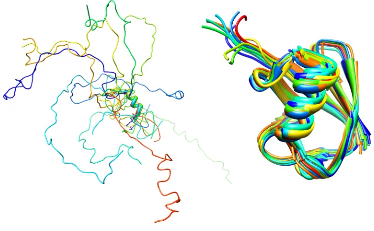
Thylakoid soluble phosphoprotein TSP9 (left, PDB id: 2FFT) and Ubiquitin (right, PDB id: 1D3Z).
The structural differences between IDPs and globular proteins (Figure 1.1) illustrate that disorder is encoded in their sequences. IDPs have different amino acid compositions than globular proteins. They are enriched in charged, polar and the structure-breaking residues, glycine and proline (1, 6). Hydrophobic and aromatic content is also lower in IDPs (1, 6). As a result, IDPs usually lack hydrophobic cores, which stabilize globular proteins. Due to the absence of hydrophobic cores, IDPs are more dynamic compared to globular proteins. Ordered regions of globular proteins undergo relatively small
fluctuations around their equilibrium backbone atom positions over time. In comparison, IDPs usually exhibit significant changes in their φ and ψ angles over time and may not have specific equilibrium values (6). Although IDPs lack stable tertiary structures, they may contain elements of secondary structure, which are often crucial for their
functionality (eg. target binding).
The dynamic properties of IDPs are intimately related to the timescale of conformational exchange within the ensemble (Figure 1.1), which govern target recognition and how these proteins function. Different structures in the ensemble can participate in the interactions with distinct targets; therefore, the rate of exchange between conformers can have significant impact on the protein function (7, 8).
1.2 Target binding by IDPs
IDPs employ to bind to their targets will aid in development of therapeutic approaches targeting these interactions (9).
Studies have shown that the unique structural properties of IDPs are important for their ability to act as hubs in PPI networks (10-12). Like proteins in the unfolded state, IDPs do not adopt completely random coil conformations (13-16). Many IDPs have considerable conformational propensities (17-19). Segments of IDPs that contain residual structure may act as molecular recognition features (MoRFs) for binding to their targets (17, 19). MoRFs are defined as 5-25 residue target binding regions, which may contain residual structure in their unbound states (17). It is possible for IDPs to contain multiple MoRFs along their sequence allowing them to interact with different binding partners. Also, binding to different targets can cause a MoRF to adopt completely different structures (17, 20, 21). For example, the same region of the intrinsically disordered N-terminal of p53 can adopt a helix or a sheet depending on its binding partners (21).
4
Figure 1.2 Mechanisms of target binding by IDPs.
Possible mechanism(s) for the interaction between the intrinsically disordered phosphorylated kinase inducible activation domain (pKID) and KIX domain of the CREB binding protein (26). Usage of this figure has been granted by the Nature Publishing Group (licence number 2993681394339).
1.3 IDPs and diseases
IDPs have been found to be associated with cancers, neurodegenerative diseases and aging (5, 27). Because their structural plasticity often allows them to interact with a large number of targets, IDPs are enriched in signaling networks (5). They have been shown to be involved in various activities, such as signal transduction, apoptosis, cell differentiation, and neuron function (28). In addition to missignalling diseases, IDPs are also involved in diseases related to protein misfolding (5). Mutations, exposure to toxins, aberrant posttranslational modifications and other factors can lead to misfolding of these
bind to their targets is poorly understood. In the case of the binding of the phosphorylated kinase inducible domain of
CREB (pKID) to the KIX domain of CBP, we find that the mechanism more nearly approximates the lower of these
two possibilities, with the formation of unstructured encounter complexes and an intermediate, partly folded complex
before formation of the final, fully folded complex.
proteins, which can have serious consequences. The term ‘misfolding’ may seem counterintuitive because IDPs do not adopt stable folds. However, in several
neurodegenerative disorders, the normal, disordered form of a protein may convert to a ‘misfolded’ conformation that is prone to aggregation. The build up of non-functional, ordered and highly stable amyloid fibrils in various tissues can result in specific pathological conditions depending on the protein (5). Because IDPs typically have low structural preferences compared to folded proteins, it is thought that they can transform into an aggregate-prone conformation more easily. Understanding the links between sequence, structure and target binding by IDPs is crucial for improving our understanding of their roles in disease and developing treatments and cures.
1.4 Techniques for characterizing IDPs
Nuclear magnetic resonance spectroscopy (NMR) and X-ray crystallography are commonly used methods to obtain atomic details of protein structure and dynamics. The dynamic nature of IDPs makes acquiring diffracting crystals of them in unbound states nearly impossible (29). Therefore, NMR is the primary technique for studying the structure and dynamics of IDPs (30, 31). NMR can yield a wealth of data, but there are limitations. Data collected by NMR are averaged over time and represent an ensemble average. For globular proteins, the protein core is stable and the ensemble average is usually a good representation of a true physical state. For highly flexible polymers, like IDPs, the ensemble average may not represent a realistic physical state. To
1.4.1 NMR spectroscopy
NMR is a technique used to determine the chemical environment of atoms (32-35). This information can be used to learn about the structure, dynamics, chemical environment, etc of the molecules that the atoms are contained in. The technique exploits the magnetic properties of specific nuclei in order to obtain this information. In a
magnetic field (Bo), NMR active nuclei, atoms that have odd number of protons, neutrons, or both, and spin values of ½ (eg. 1H, 15N, 13C) will precess in either aligned or opposed orientations parallel to the field (Figure 1.3). Nuclei in the spin-aligned state have a slightly lower energy and are slightly more populated than the spin opposed nuclei. By applying electromagnetic radiation, in the form of radio waves, these nuclei can be temporarily be excited to the higher energy, unaligned state. Data collected during the return to the lower energy state gives information about the local environment of the nuclei (chemical shift). This is the basis of all NMR experiments. Various types and patterns of electromagnetic pulses are combined to generate specific NMR
experiments to obtain the desired information (eg. chemical environment, dynamics, etc) about the nuclei.
NMR can be used to determine protein structures and numerous other properties, such as dynamics. The process of determining a protein structure by NMR can be divided into two parts: assignment and restraint collection. Assignment refers to the
determination of the chemical shift values of spin ½ nuclei. Next, restraints are gathered (distances, angles, orientations, etc) for the assigned atoms, which are used to
computationally fold the polypeptide in such a way that the restraints are satisfied. The two steps are not always mutually exclusive. For example, through space distance restraints may be also used to assist with or verify the resonance assignment. For small proteins and peptides (~30 residues or less), homonuclear NMR experiments (eg. 1H signals only) may be sufficient to assign the proton resonances (via 1H-1H COSY and TOCSY experiments) and determine the structure (via 1H-1H NOESY). This approach is used in chapter 4 to assign and collect distance restraints for several ~20-mer peptides. Due to spectral crowding and overlap in the 1H dimension, multidimensional,
proteins and peptides. In chapter 5, several heteronuclear experiments were used to assign backbone resonances for a ~32 kDa protein domain. In this case, the goal of assignment was not to determine the structure. Instead, we used the assigned 1H-15N HSQC spectrum to determine the residue-specific chemical shift changes upon addition of a peptide from a binding partner. This allowed us to map the binding interface (chemical shift mapping) onto a previously determined crystal structure. Furthermore, assignment of the 13Cα and
13C
β resonances allowed for the determination of secondary structure content of the
polypeptide. NMR can also be used to study protein dynamics. Relaxation measurements allow one to determine motions occurring on ps-ns timescales, which can help to identify structured and flexible regions of proteins. These types of experiments are employed in chapter 6 to measure changes in the dynamics of IDPs under crowded conditions. The experiments mentioned here are just a few examples of the uses of NMR.
Figure 1.3 The basis of NMR experiments.
higher energy state. Data collected as the nuclei return to equilibrium gives information about the local environment of the nuclei.
1.4.2 MD simulations
MD is a simulation of the movement of particles, accomplished by solving Newton’s equation of motion (2nd law) for a system of interacting particles:
€
F i=mia i=mid v i dt =mi
d2 r
i dt2
Where Fi is the force exerted on particle i, mi is the mass of particle i, ai is the
acceleration of particle i, vi is the velocity of particle i and ri is the position of particle i at
time t.
Using this equation, a trajectory (particle positions as a function of time) can be calculated by integration once the initial positions and velocities of the particles are known. The positions may come from a known structure (eg. Crystal or NMR protein structure) and the velocities are often taken from a Maxwellian distribution at the desired temperature. From these values, the forces on the particles (usually atoms) are calculated. The particles are allowed to move for a short period of time (the timestep), and
integration gives their t+1 positions. Time is moved forward according to the timestep. This process is repeated as long as necessary. A number of different integration
algorithms may be used, such as leap frog and velocity Verlet (36, 37).
The calculation of forces is the most time-consuming process in the generation of a trajectory. The forces may also be expressed as the negative gradient of the potential energy:
€
The potential energy function (V) is the sum of terms for bonded and non-bonded energies. These energies are determined as a function of the atom positions (Cartesian coordinates, r) in the system:
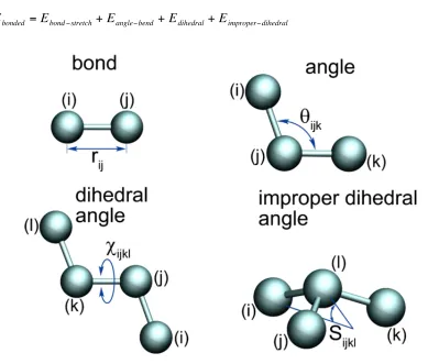
The bonded interactions typically contain terms for stretching, angle-bending, dihedral angle and, usually, a term for improper dihedral angles, which functions to maintain the planarity of planar molecules (Figure 1.4):
Figure 1.4 Bonded energy terms for MD simulations.
Figure usage granted under MesoBioNano (MBN) explorer academic license agreement (http://www.mbnexplorer.com/academic-license-agreement) (38).
!
V(r)=Ebonded +Enon"bonded
!
The non-bonded energy consists of terms for Van der Waals and electrostatic interaction energies. Van der Waals forces are approximated using the Lennard-Jones potential:
Where ε is the well depth, σ is the distance where the inter-particle potential is zero and r is the distance between the particles. Figure 1.5 illustrates examples of Lennard-Jones potentials.
Figure 1.5 Examples of Lennard-Jones potentials.
r is the distance between particles in nanometers and the Lennard-Jones potential is given in kJ/mol. All Lennard-Jones potentials include repulsive and attractive components. Here, the grey curve has a greater attractive component compared to the black one.
The Coulomb interactions between two charged particles is given by:
!
VLJ =4" #
!
VC(rij)= qiqj
4"#o#rrij
Where q is the charge on each particle,
!
"r is the relative dielectric constant and rij is the
separation distance.
The values associated with each of the energy terms are dictated by the force field being used for the simulation. Chapter 2 details some of the most commonly used force fields for biomolecular simulations.
When conducting MD simulations of biomolecules, such as proteins, it is usually desirable to mimic experimental, or laboratory conditions (eg. temperature, pressure). Direct integration of Newton’s equation of motion will result in the system energy being conserved, which corresponds to an isolated system. In contrast, laboratory experiments are typically “open” systems. To reproduce experimental conditions it is usually desirable to run simulations under the NPT ensemble, where the number of particles, pressure and temperature of the system are kept constant. This is accomplished by coupling the system to temperature and/or pressure baths. Thermostat (39, 40) and barostat (41-44) algorithms can be employed to achieve the NPT ensemble.
One final concept that warrants introduction is that of periodic boundary
Figure 1.6 Periodic boundary conditions in 2D.
The system (center) is surrounded by translated copies of itself, eliminating edge effects and mimicking a bulk solvent environment (45). Figure usage granted under the GNU General Public License (http://www.gnu.org/copyleft/gpl.html).
MD simulations have become increasingly valuable tools in the field of biochemistry. Berni Alder invented the technique in the late 1950’s and in 1959
performed the first MD simulation – of a group of interacting hard spheres under periodic boundary conditions (46). The first protein MD simulation was performed in 1975 of the bovine pancreatic trypsin inhibitor (BPTI) (47). Since then, advances in computing power have allowed for MD simulations to be used to study considerably more complex
systems. They have become important predictive tools. Today, MD simulations are routinely used for NMR structure determination, refining X-ray crystal structures, protein-ligand docking, drug discovery/refinement, protein folding and countless other purposes. As computational power and software algorithms improve, the uses and applications of MD simulations will expand correspondingly.
1.4.3 ITC
ITC is a method to quantitatively measure the thermodynamic parameters of interactions in solution (48). The binding affinity (Ka), enthalpy changes (ΔH) and stoichiometry (n) of the interaction between two or more molecules are measured
j’ j’ i’ i’ i’ i’ j’ i’ i’ y x y x j’ j’ i’ i’ i’ i j’ j’ j’ j’ i’ i i’ j’ j’ j’ j i’ i’ i’ j’ i’ i’ j’ j’ j’ j
Figure 3.1: Periodic boundary conditions in two dimensions.
better suited to the study of an approximately spherical macromolecule in solution, since fewer solvent molecules are required to fill the box given a minimum distance between macromolecular images. At the same time, rhombic dodecahedra and truncated octahedra are special cases of
triclinicunit cells; the most general space-filling unit cells that comprise all possible space-filling
shapes [18]. For this reason, GROMACS is based on the triclinic unit cell.
GROMACS uses periodic boundary conditions, combined with theminimum image convention:
only one – the nearest – image of each particle is considered for short-range non-bonded in-teraction terms. For long-range electrostatic inin-teractions this is not always accurate enough, and GROMACS therefore also incorporates lattice sum methods such as Ewald Sum, PME and PPPM. GROMACS supports triclinic boxes of any shape. The simulation box (unit cell) is defined by the 3 box vectorsa,bandc. The box vectors must satisfy the following conditions:
ay =az =bz = 0 (3.1)
ax >0, by >0, cz >0 (3.2)
|bx| ≤ 1
2ax, |cx| ≤ 1
2ax, |cy| ≤ 1
2by (3.3)
Equations3.1can always be satisfied by rotating the box. Inequalities (3.2) and (3.3) can always be satisfied by adding and subtracting box vectors.
directly. Determination of these parameters allows one to derive the Gibbs free energy and entropy changes (ΔG and ΔS, respectively) using the relationship:
Where R is the gas constant and T is the temperature.
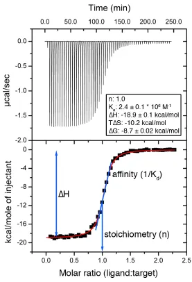
Briefly, in an ITC experiment, a binding target is loaded into the sample cell and subjected to a stepwise titration of precise volumes of ligand into the same cell (Figure 1.7). The reference cell contains water or buffer. A constant power is applied to the reference cell heater. During the titration, sensitive thermocouples measure the temperature differences between the reference and sample cells. In an exothermic
reaction, heat is evolved in the sample cell and the power to the heater is decreased. In an endothermic reaction, heat is absorbed in the sample cell and the heater is activated. The heat input required to maintain the same temperatures in the sample and reference cells is measured throughout the experiment (Figure 1.8). Integration of the heat input with respect to time as a function of the molar ratio ((ligand)/(target)) gives the
thermodynamic parameters of interest.
!
Figure 1.7 ITC instrument schematic.
Figure 1.8 Typical ITC data
The top panel shows the raw ITC data and the bottom panel shows the binding isotherm.
1.5 Significance and aims
Figure 1.9 The structure of the Kelch domain of Keap1 and its interaction with the Neh2 domain of Nrf2.
Two-site binding is disrupted under conditions of oxidative stress preventing Nrf2 degradation and allowing promotion of cytoprotective gene expression. The structure corresponding to PDB id 1X2R was obtained from (67) and rendered with VMD (68).
1.6 Thesis outline
parameters and force field selection for performing MD simulations of IDPs. This was accomplished by performing extensive MD simulations of a peptide from the high affinity motif of Nrf2 with 10 different force fields and different parameters. The results were compared to experimental data. After determining suitable combinations of
parameters for simulating IDPs, we applied the methodology to more diverse IDP systems. In chapters 3 and 4, we combine MD simulations with experimental techniques to dissect the mechanisms used by 9 different IDPs for binding to a common target, the Kelch domain of Keap1. Our findings provide valuable insights into the mechanisms used by IDPs for target binding and should also help to elucidate the biological roles of the various protein-protein interactions. In chapter 5, we report the backbone resonance assignments for the Kelch domain of Keap1 and map its binding interface with a peptide from the high affinity motif of Nrf2. This study was important for examining IDP binding from the perspective of a target, allowing us to more thoroughly understand IDP
interactions. Chapter 6 focuses on determining how molecular crowding affects the dynamics of IDPs. Inside cells, the concentration of macromolecules can reach up to 400 g/L. In such crowded environments, proteins are expected to behave differently than in vitro. The dynamic properties of IDPs are intimately related to the timescale of
conformational exchange within the ensemble, which govern target recognition and how these proteins function. Therefore, assessing how these properties are affected by
1.7 References
1. Dunker AK et al. (2001) Intrinsically disordered protein. J Mol Graph Model 19:26-59.
2. Wright PE, Dyson HJ (1999) Intrinsically unstructured proteins: re-assessing the protein structure-function paradigm. J Mol Biol 293:321-31.
3. Dunker AK et al. (1998) Protein disorder and the evolution of molecular recognition: theory, predictions and observations. Pac Symp Biocomput 473-84.
4. Dunker AK, Obradovic Z, Romero P, Garner EC, Brown CJ (2000) Intrinsic protein disorder in complete genomes. Genome Inform Ser Workshop Genome Inform 11:161-71.
5. Uversky VN, Oldfield CJ, Dunker AK (2008) Intrinsically disordered proteins in human diseases: introducing the D2 concept. Annu Rev Biophys 37:215-46.
6. Radivojac P et al. (2007) Intrinsic disorder and functional proteomics. Biophys J 92:1439-56.
7. Mittag T, Kay LE, Forman-Kay JD (2010) Protein dynamics and conformational disorder in molecular recognition. J Mol Recognit 23:105-16.
8. Smock RG, Gierasch LM (2009) Sending signals dynamically. Science 324:198-203.
9. Cheng Y et al. (2006) Rational drug design via intrinsically disordered protein. Trends Biotechnol 24:435-42.
10. Patil A, Nakamura H (2006) Disordered domains and high surface charge confer hubs with the ability to interact with multiple proteins in interaction networks. FEBS Lett 580:2041-5.
12. Haynes C et al. (2006) Intrinsic disorder is a common feature of hub proteins from four eukaryotic interactomes. PLoS Comput Biol 2:e100.
13. Gall C, Xu H, Brickenden A, Ai X, Choy WY (2007) The intrinsically disordered TC-1 interacts with Chibby via regions with high helical propensity. Protein Sci 16:2510-8.
14. Choy WY, Forman-Kay JD (2001) Calculation of ensembles of structures representing the unfolded state of an SH3 domain. J Mol Biol 308:1011-32.
15. Morar AS, Olteanu A, Young GB, Pielak GJ (2001) Solvent-induced collapse of alpha-synuclein and acid-denatured cytochrome c. Protein Sci 10:2195-9.
16. Shortle D, Ackerman MS (2001) Persistence of native-like topology in a denatured protein in 8 M urea. Science 293:487-9.
17. Mohan A et al. (2006) Analysis of molecular recognition features (MoRFs). J Mol Biol 362:1043-59.
18. Sigalov AB, Zhuravleva AV, Orekhov VY (2007) Binding of intrinsically disordered proteins is not necessarily accompanied by a structural transition to a folded form. Biochimie 89:419-21.
19. Fuxreiter M, Simon I, Friedrich P, Tompa P (2004) Preformed structural elements feature in partner recognition by intrinsically unstructured proteins. J Mol Biol 338:1015-26.
20. Dunker AK, Cortese MS, Romero P, Iakoucheva LM, Uversky VN (2005) Flexible nets. The roles of intrinsic disorder in protein interaction networks. FEBS J 272:5129-48.
21. Oldfield CJ et al. (2008) Flexible nets: disorder and induced fit in the associations of p53 and 14-3-3 with their partners. BMC Genomics 9 Suppl 1:S1.
23. Tsai CJ, Ma B, Sham YY, Kumar S, Nussinov R (2001) Structured disorder and conformational selection. Proteins 44:418-27.
24. Kumar S, Ma B, Tsai CJ, Sinha N, Nussinov R (2000) Folding and binding cascades: dynamic landscapes and population shifts. Protein Sci 9:10-9.
25. Espinoza-Fonseca LM (2009) Reconciling binding mechanisms of intrinsically disordered proteins. Biochem Biophys Res Commun 382:479-82.
26. Sugase K, Dyson HJ, Wright PE (2007) Mechanism of coupled folding and binding of an intrinsically disordered protein. Nature 447:1021-5.
27. Iakoucheva LM, Brown CJ, Lawson JD, Obradović Z, Dunker AK (2002) Intrinsic disorder in cell-signaling and cancer-associated proteins. J Mol Biol 323:573-84.
28. Raychaudhuri S, Dey S, Bhattacharyya NP, Mukhopadhyay D (2009) The role of intrinsically unstructured proteins in neurodegenerative diseases. PLoS One 4:e5566.
29. Dyson HJ, Wright PE (2005) Intrinsically unstructured proteins and their functions. Nat Rev Mol Cell Biol 6:197-208.
30. Eliezer D (2009) Biophysical characterization of intrinsically disordered proteins. Curr Opin Struct Biol 19:23-30.
31. Mittag T, Forman-Kay JD (2007) Atomic-level characterization of disordered protein ensembles. Curr Opin Struct Biol 17:3-14.
32. Rule GS, and Hitchens TK (2005) Fundamentals of protein NMR spectroscopy (Springer).
33. Rabi II, Zacharias JR, Millman S, Kusch P (1992) Milestones in magnetic resonance: 'a new method of measuring nuclear magnetic moment' . 1938. J Magn Reson Imaging 2:131-3.
35. Bloch F, Hansen WW, Packard M (1946) Nuclear induction Phys Rev 70:460-474.
36. Swope WC, Andersen HC, Berens PH, Wilson KR (1982) A computer simulation method for the calculation of equilibrium constants for the formation of physical clusters of molecules: Application to small water clusters. J Chem Phys 76:637.
37. Berendsen HJC, and van Gunsteren WF (1986) in Molecular-Dynamics Simulation of Statistical-Mechanical Systems (North-Holland, Amsterdam), p 43-65.
38. Solov'yov IA, Yakubovich AV, Nikolaev PV, Volkovets I, Solov'yov AV (2012) MesoBioNano explorer-A universal program for multiscale computer simulations of complex molecular structure and dynamics. J Comput Chem (in press).
39. Berendsen HJC, Postma JPM, Van Gunsteren WF, DiNola A, Haak JR (1984) Molecular dynamics with coupling to an external bath. J Chem Phys 81:3684-3690.
40. Bussi G, Donadio D, Parrinello M (2007) Canonical sampling through velocity rescaling. J Chem Phys 126:014101.
41. Hoover WG (1985) Canonical dynamics: Equilibrium phase-space distributions. Phys Rev A 31:1695-1697.
42. Nose S, Klein ML (1983) Constant pressure molecular dynamics for molecular systems. Mol Phys 50:1055-1076.
43. Nosé S (1984) A molecular dynamics method for simulations in the canonical ensemble. Mol Phys 52:255-268.
44. Parrinello M, Rahman A (1981) Polymorphic transitions in single crystals: A new molecular dynamics method. J Appl Phys 52:7182-7190.
46. Alder BJ, Wainwright TE (1959) Studies in molecular dynamics. I. General method. J Chem Phys 31:459-466.
47. Levitt M, Warshel A (1975) Computer simulation of protein folding Nature 253:694.
48. Pierce MM, Raman CS, Nall BT (1999) Isothermal titration calorimetry of protein-protein interactions. Methods 19:213-221.
49. Itoh K et al. (1999) Keap1 represses nuclear activation of antioxidant responsive elements by Nrf2 through binding to the amino-terminal Neh2 domain. Genes Dev 13:76-86.
50. Li X, Zhang D, Hannink M, Beamer LJ (2004) Crystal structure of the Kelch domain of human Keap1. J Biol Chem 279:54750-8.
51. Tong KI, Kobayashi A, Katsuoka F, Yamamoto M (2006) Two-site substrate
recognition model for the Keap1-Nrf2 system: a hinge and latch mechanism. Biol Chem 387:1311-20.
52. Lo SC, Li X, Henzl MT, Beamer LJ, Hannink M (2006) Structure of the Keap1:Nrf2 interface provides mechanistic insight into Nrf2 signaling. EMBO J 25:3605-17.
53. Lo SC, Hannink M (2006) PGAM5, a Bcl-XL-interacting protein, is a novel substrate for the redox-regulated Keap1-dependent ubiquitin ligase complex. J Biol Chem
281:37893-903.
54. Tong KI et al. (2006) Keap1 recruits Neh2 through binding to ETGE and DLG motifs: characterization of the two-site molecular recognition model. Mol Cell Biol 26:2887-900.
55. Padmanabhan B, Nakamura Y, Yokoyama S (2008) Structural analysis of the
56. Tong KI et al. (2007) Different electrostatic potentials define ETGE and DLG motifs as hinge and latch in oxidative stress response. Mol Cell Biol 27:7511-21.
57. Li Y, Paonessa JD, Zhang Y (2012) Mechanism of chemical activation of Nrf2. PLoS One 7:e35122.
58. Sporn MB, Liby KT (2012) NRF2 and cancer: the good, the bad and the importance of context. Nat Rev Cancer 12:564-71.
59. Zhang Y, Gordon GB (2004) A strategy for cancer prevention: stimulation of the Nrf2-ARE signaling pathway. Mol Cancer Ther 3:885-93.
60. Strachan GD et al. (2004) Fetal Alz-50 clone 1 interacts with the human orthologue of the Kelch-like Ech-associated protein. Biochemistry 43:12113-22.
61. Kim JE et al. (2010) Suppression of NF-kappaB signaling by KEAP1 regulation of IKKbeta activity through autophagic degradation and inhibition of phosphorylation. Cell Signal 22:1645-54.
62. Komatsu M et al. (2010) The selective autophagy substrate p62 activates the stress responsive transcription factor Nrf2 through inactivation of Keap1. Nat Cell Biol 12:213-23.
63. Niture SK, Jaiswal AK (2011) INrf2 (Keap1) targets Bcl-2 degradation and controls cellular apoptosis. Cell Death Differ 18:439-51.
64. Tian H et al. (2012) Keap1: One stone kills three birds Nrf2, IKKβ and Bcl-2/Bcl-xL. Cancer Lett 325:26-34.
65. Camp ND et al. (2012) Wilms Tumor Gene on X Chromosome (WTX) Inhibits Degradation of NRF2 Protein through Competitive Binding to KEAP1 Protein. J Biol Chem 287:6539-50.
67. Padmanabhan B et al. (2006) Structural basis for defects of Keap1 activity provoked by its point mutations in lung cancer. Mol Cell 21:689-700.
2 Comparison of secondary structure formation using 10 different force fields in microsecond molecular dynamics simulations
Elio A. Cino†, Wing-Yiu Choy†* and Mikko Karttunen‡*
Department of Biochemistry†, 1151 Richmond St. North, The University of Western Ontario, London, Ontario, Canada N6A 5C1, Department of Chemistry‡, 200 University Avenue West, University of Waterloo, Waterloo, Ontario, Canada N2L 3G1
*Corresponding authors: [email protected], [email protected]
Citation: Cino, E. A., Choy, W. Y., & Karttunen, M. (2012). Comparison of secondary structure formation using 10 different force fields in microsecond molecular dynamics simulations. Journal of Chemical Theory and Computation, 8(8), 2725-2740
2.1 Abstract
We have compared molecular dynamics (MD) simulations of a β-hairpin forming peptide derived from the protein Nrf2 with ten biomolecular force fields using trajectories of at least one microsecond long. The total simulation time was 37.2 microseconds. Previous studies have shown that different force fields, water models, simulation methods and parameters can affect simulation outcomes. The MD simulations were done in
2.2 Introduction
Atomistic molecular dynamics (MD) simulations are a versatile tool for studying protein folding and function. They can provide detailed atomistic information, which may be difficult to obtain by experimental techniques. Increases in computational power have allowed for simulations to reach experimentally relevant time scales at the microsecond level: MD simulations have been used to study the folding of peptides and small proteins (1-9) and to model other biological systems. The current record for an atomistic
simulation of protein conformational changes, as far as we know, is 1 ms reached by Shaw et al. (7) for the 58-residue protein BPTI.
One of the major challenges in protein folding simulations is choosing an appropriate force field, see e.g. Ref (10). This is due to possible biases different force fields have towards certain types of secondary structure (3, 11-14). Ideally, the force field should be fully validated with experimental data, but that is typically not possible as it would involve validation against different structures and other physical properties from a large number of independent and fully validated experiments – mission impossible since experiments have their own error sources due to, e.g., instrumentation. While a
completely transferable force field does not exist, modifications of existing force fields have led to improvements in agreement with experimental data (15-22).
In this work, we compared 10 biomolecular force fields with respect to the folding of a peptide derived from Nuclear factor erythroid 2-related factor 2 (Nrf2). Nrf2 is an important transcription factor that regulates the expression of genes responsive to
free-state of Neh2 (30, 31). Other experimental data has shown that a peptide containing residues 74-87 can compete with the full-length Nrf2 for binding Keap1 (31). Here, we chose to use a 16-mer human Nrf2 peptide with the sequence
72AQLQLDEETGEFLPIQ87 for our MD simulations. This peptide contains the ‘ETGE’
motif and should be of sufficient length to form the necessary interactions to stabilize the β-hairpin structure. It is noteworthy that the phosphorylation of Thr-80 has been shown to impair the binding to Keap1(31). Since Neh2 is largely disordered and lacks a tertiary structure, this β-hairpin likely folds independently, making it a good target for folding simulations (30).
In addition to Nrf2, several other proteins that contain ‘ETGE’-like motifs have been shown to interact with the Kelch domain of Keap1. These include PGAM5 (32), FAC1 (33), PTMA (34), p62 (35), WTX (36) and PALB2 (37). Some of these Keap1 interacting proteins have only been recently discovered, which suggests that this list of targets may still be growing. Structures of PTMA (Prothymosin alpha) and p62 peptides in complex with Keap1 indicate that their ‘ETGE’-like motifs bind to the same region as the ‘ETGE’ motif of Nrf2 and form similar hairpin structures in their bound states (31, 34, 35). Interestingly, MD simulations from our previous work showed that the binding motifs of Nrf2 and PTMA have tendency to form hairpin structures that resembled the bound state conformation even in the absence of Keap1 (9). With the list of Keap1 binding partners seemingly expanding and MD simulations becoming an increasingly important and predictive tool, it is important to establish appropriate simulation protocols for these systems, including force field choice.
β-hairpins are a type of protein supersecondary structure consisting of two
molecular dynamics simulations using 10 different force fields (details in next section). We selected these force fields primarily because they are commonly used in biomolecular simulations, including those of β-hairpin folding (3, 9, 41, 42).
Force field selection is a key factor in the outcome of protein folding simulations. Although force field modifications have led to improved agreements between MD simulations and experimental data, continued testing and comparison with experimental data is required to further these advances. While studies comparing different force fields have been conducted previously, very few of them had included such a large set of force fields with respect to folding of secondary structure elements (3, 14, 19, 43-45).Small proteins and peptides with folding times on the microsecond timescale are excellent systems to test and compare force fields; such trajectories provide reasonable sampling of conformations and sufficient length to examine the stability of the force field.
In this work, we compare MD simulations of a β-hairpin forming peptide derived from the protein Nrf2, performed with ten force fields. We assess their agreements with experimental data. The effects of elevated temperatures, charge-groups (46, 47), peptide capping and phosphorylation of Thr-80 with respect to β-hairpin formation were also examined. Despite using identical starting structures and simulation parameters, we observed clear differences amongst the various force fields and even between replicate simulations using the same force field. Such a comprehensive comparison will offer useful guidance to others conducting similar types of simulations and for improving force fields.
2.3 Simulation methodology
(31). The exact same starting structure was used for all simulations. For the
phosphorylated peptide (pThr-80) simulations, a dianionic phosphate group (PO42-) was modeled onto residue Thr-80 of the same structure using chimera (49).
Force fields
We compared the peptide folding using the following force fields: Amber ff99SB-ILDN (15, 19, 20), Amber ff99SB*-ff99SB-ILDN (15, 17, 19, 20), Amber ff99SB (15, 19), Amber ff99SB* (15, 17, 19), Amber ff03 (15, 16), Amber ff03* (15-17), GROMOS96 43a1p (50, 51), GROMOS96 53a6 (21, 22), CHARMM27 (version c32b1) with CMAP (18, 52, 53) and OPLS-AA/L force fields (54-56). The ‘*’ designations on the Amber force fields indicate the presence of a modification to the backbone dihedral potentials to improve agreement with experimental data (17). The ‘ILDN’ designation indicates the presence of a modification to the side-chain torsion potentials of isoleucine, leucine, aspartate and asparagine to improve agreement with quantum-mechanical calculations (20). Combination of the ‘ILDN’ and ff99SB* modifications has been demonstrated recently (44, 57). For a recent summary of the evolution of the Amber ff99 and ff03 series of force fields see the results section of (44) The ‘p’ designation on the GROMOS96 43a1 force field indicates the inclusion of phosphorylated amino acid parameters to the otherwise unmodified 43a1 parameters (50). One major difference between the GROMOS force fields and the others used in this study is that the GROMOS force fields are united atom and do not explicitly have all hydrogen atoms. The ‘AA’ and ‘/L’ designations on the OPLS force field indicate all-atom and the inclusion of updated dihedral parameters from the original distribution(56).
Phosphothreonine parameters included in the CHARMM27 force field distribution were used (18, 53).
Simulation details
A. General parameters. Simulations were performed using GROMACS
(GROningen MAchine for Chemical Simulations) version 4.5 (47) Although GROMACS was used in this work, we expect that our findings will be applicable to other simulation software that utilizes the same force fields (59). Cubic boxes of linear size 6 nm were used and periodic boundary conditions were applied in all directions. Sodium (Na+) and chloride (Cl-) ions were added to neutralize the system and bring the salt concentration to 0.1 M. Na+ and Cl- parameters specific to each force field distribution were used (60). Protein and non-protein atoms were coupled to their own temperature baths, which were kept constant at 310 K using the Parrinello-Bussi algorithm (61). This approach has been shown to perform very well in biomolecular simulations (46). Pressure was maintained isotropically at 1 bar using the Parrinello-Rahman barostat (62). A 2-fs timestep was employed. Prior to the production runs, the energy of each system was minimized using the steepest descents algorithm. This was followed by 2 ps of position-restrained
dynamics with all non-hydrogen atoms restrained with a 1000 kJ mol-1 force constant. Initial atom velocities were taken from a Maxwellian distribution at 310 K. All bond lengths were constrained using the LINCS algorithm (63). A 1.0 nm cut-off was used for Lennard-Jones interactions. Dispersion corrections for energy and pressure were applied. Electrostatic interactions were calculated using the Particle-Mesh Ewald (PME) method (64) with 0.12 nm grid-spacing and a 1.0 nm real-space cut-off. No reaction-field or cutoff methods were tested as they have previously been shown be inferior to PME (65, 66). System coordinates were written out at 4 ps intervals during the production runs.
unphysical charges introduced by the free N- and C-termini, which can potentially disrupt the native structure. To study the effects of peptide capping, several simulations with the N- and C-terminus capped with acetyl (ACE) and NH2 groups, respectively, were
performed (Table 2.1). The starting structure was solvated in SPC (simple point charge), TIP3P or TIP4P (67, 68) water. The compatibility of these water models with ions has been examined in detail by (60). A three-point water model (SPC or TIP3P) was recommended by GROMACS for all of the force fields used in this study, with the exception of OPLS-AA/L, in which the four-point (TIP4P) water model was the
recommended choice (Table 2.1). Simulations with TIP3P and TIP4P were conducted for this force field (Table 2.1). The non-phosphorylated peptide systems each contained 17 Na+ and 13 Cl- ions, while for the pThr-80 systems two extra Na+ ions were added to
neutralize the dianionic phosphate group. For each force field, a simulation was conducted without the use of charge-groups (single atom charge groups); GROMACS uses the concept of charge groups to speed up simulations, see section “Domain Decomposition” in (47) for details. It has recently been shown that in some situations charge-groups can lead to pronounced unphysical effects (46). To examine the effect of charge-groups, additional simulations were conducted with the GROMOS96 and OPLS-AA/L force fields employing the default charge-groups for these force fields. Simulations performed with charge-groups are denoted with brackets around the force field name in the results section. For simulations conducted with the CHARMM27 force field, CMAP correction was applied (18). A few of the simulations were duplicated in order to assess reproducibility (Table 2.1). These systems did not use charge-groups, were prepared in the same manner as stated above and were assigned different initial atom velocities than their originals. Duplicated simulations are denoted with bracketed sequential numbering beside the force field name in the results section. We also performed elevated
temperature simulations at 330, 350 and 370K with the Amber ff99SB*-ILDN (15, 17, 19, 20), Amber ff03*, (15-17) GROMOS96 53a6, (21, 22) CHARMM27 with CMAP (18, 52, 53) and OPLS-AA/L force fields (54-56). Using the initial and final (after 1 µs) system configurations at 310K, we reassigned the atom velocities at each higher
In total, 28 individual 1 µs simulations were conducted and two of these
trajectories were extended to 2 µs (Amber ff99SB* and OPLS-AA/L). An additional 7.2 µs of simulations at elevated temperature were performed. The cumulative simulation time was 37.2 µs. The simulations are summarized in Table 2.1.
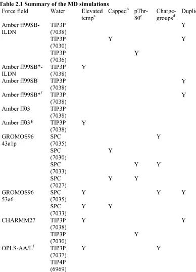
Table 2.1 Summary of the MD simulations
Force field Water Elevated tempa
Cappedb pThr-80c
Charge-groupsd
Duplicatee
Amber
ff99SB-ILDN TIP3P (7038) Y
TIP3P (7030)
Y Y
TIP3P
(7036) Y
Amber ff99SB*-ILDN
TIP3P
(7038) Y Amber ff99SB TIP3P
(7038) Y
Amber ff99SB*f TIP3P
(7038) Y
Amber ff03 TIP3P (7038) Amber ff03* TIP3P
(7038) Y GROMOS96 43a1p SPC (7035) Y SPC (7030) Y SPC
(7033) Y Y
SPC (7027)
Y Y
GROMOS96 53a6
SPC (7035)
Y Y Y
SPC (7033)
Y Y
CHARMM27 TIP3P
(7038)
Y Y
TIP3P
(7030) Y
OPLS-AA/Lf TIP3P (7037)
Y Y
a ‘Y’ indicates that elevated temperature simulations were performed at 330, 350 and 370 K from the initial and final (after 1µs) system configurations.
b ‘Y’ indicates that the N and C termini of the peptide was capped with with acetyl (ACE) and NH2 groups, respectively. They were otherwise left uncapped (NH3+ and COO-, respectively).
c ‘Y’ indicates that residue Thr-80 was phosphorylated.
d ‘Y’ indicates that two simulations were performed: one with default GROMACS charge-groups and one without charge-groups.
e ‘Y’ indicates that two simulations, each 1 µs, were performed. Duplicates were always performed without charge-groups and were identical to the first simulation except for their initial atom velocities.
f The trajectory was extended to 2 µs.
Simulation analysis
We used either the full 1 µs trajectories or the last 0.1 µs for analysis. By restricting some analyses to the last 0.1 µs, we allowed as much time as possible for the simulations to converge to a stable conformation. Hydrogen bonds were analyzed as follows: A hydrogen bond betweena donor (D-H) and an acceptor (A) wasconsidered to be formed when the DA distance was less than3.2 Å and the angle between the DA vector andthe D-H bond (AD-H angle) was less than 35°. These geometric criteria for defining hydrogen bonds are consistent with those used in prior studies (69, 70). Secondary structure content was assessed with the DSSP algorithm (71).
2.4 Results
We have compared the secondary structures and free- and bound-state contact formations in MD simulations of a β-hairpin forming peptide derived from the
intrinsically disordered Neh2 domain of Nrf2 conducted with 10 different biomolecular force fields. The DSSP algorithm was used to monitor the evolution of secondary structures over the entire 1 µs trajectories. β-hairpin formation was identified by inspection of the cluster center structures and the Cα-Cα atom pair distances during the
RMSDs and backbone dihedral angles in the MD structures to the peptide in complex with its binding target, Keap1 (31). The effects of elevated temperatures, terminal capping, charge-groups and phosphorylation of Thr-80 on hairpin folding were also assessed.
Assessing secondary structure formation at 310K
To compare the MD trajectories obtained with different force fields, we first
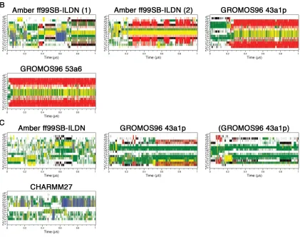
Figure 2.1 Secondary structure propensity analysis of the trajectories.
Secondary structure content was assessed with the DSSP algorithm(71): coil (white), β-sheet (red), β-bridge (black), bend (green), turn (yellow), α-helix (blue) and 310 helix (grey). A) Uncapped peptide. B) Capped peptide. C) pThr-80
Figure 2.2 Cluster centroid structures from the last 0.1 µs of the simulations.
A single cluster represented all structures in each simulation and the center structure was extracted. A) Uncapped peptide. B) Capped peptide. C) pThr-80 peptide.
There were clear differences between replicate runs using the same force fields. Specifically, the Amber ff99SB-ILDN (2), Amber ff99SB (1) and Amber ff99SB* (1) simulations did not converge upon β-hairpin conformations (Figures 2.1A & 2.2A). To determine if a longer trajectory would lead to hairpin formation, we extended the Amber ff99SB* (1) simulation to 2 µs. DSSP analysis, however, still was not indicative of a hairpin structure (data not shown).
were differences between the two Amber ff99SB-ILDN replicates. While the Amber ff99SB-ILDN (1) simulation did have turn and strand contents in the expected region, it appeared to be transient and not as pronounced as the Amber ff99SB-ILDN (2) hairpin signature (Figure 2.1B). Figure 2.2B shows that close to the end of the trajectory, Amber ff99SB-ILDN (1) structure adopted a short non-native helix before the turn region while hairpin structure that is slightly displaced from the expected location was observed in the Amber ff99SB-ILDN (2) trajectory.
The phosphorylation of Thr-80 located at the turn region appears to have significant effects on the peptide folding. β-hairpin formation was not observed in any of the pThr-80 simulations (Figures 2.1C & 2.2C). Interestingly, these simulations all displayed considerable bend content but failed to form a turn in the expected location (Figure 2.1C).
The averaged Cα-Cα atom pair distances (within 10 Å) were also plotted to identify
β-hairpin formation in the simulations (Figure 2.3). In these plots, the β-turn (77DEET80) region, which the hairpin is approximately centered around, was indicated. For the uncapped peptides, the Amber ff99SB-ILDN (1), Amber ff99SB*-ILDN, Amber ff99SB (2), Amber ff99SB* (2), Amber ff03, Amber ff03*, GROMOS96 43a1p and
GROMOS96 53a6 (1 & 2) simulations, including those which used charge-groups, appeared to form β-hairpins as evidenced by the cross-strand Cα-Cα contacts centered
around the β-turn (Figure 3.3A). Like the DSSP plots, this analysis also revealed clear differences between the replicates of Amber ff99SB-ILDN, Amber ff99SB, and Amber ff99SB* simulations. While Amber ff99SB-ILDN (2) displayed no signature of β-hairpin structure, the hairpins formed in the Amber ff99SB (1) and Amber ff99SB* (1)
simulations were found in different regions compared to the replicas (Figure 2.3A). The CHARMM27 simulations did not have cross-strand Cα-Cα contacts indicative of β
-hairpin structures, but showed regions of compactness in the turn segment (Figure 2.3A). The OPLS-AA/L simulations without charge groups had some evident cross-strand contacts, but the β-turn was shifted from the expected location (Figure 2.3A); while the OPLS-AA/L simulation with default charge-groups did not appear to form a hairpin (Figure 2.3A). Cα-Cα contacts in the capped peptide simulations were indicative of
fields, the β-hairpin in the Amber ff99SB-ILDN simulations were shifted from the expected location (Figure 2.3B). None of the pThr-80 simulations had cross-strand
contacts evident of β-hairpin structures (Figure 2.3C). It is worthwhile to note that in both GROMOS96 43a1p trajectories with Thr-80 phosphorylated there was evidence of close contacts between the positively charged N-terminus and the negatively charged
Figure 2.3 Cα-Cα atom pair distances.
Average Cα-Cα distances less than or equal to 10 Å during the last 0.1 µs of the
MD simulations. Distances equal to or greater than 10 Å are colored blue. The black square indicates the β-turn (77DEET80) region. A) Uncapped peptide. B) Capped peptide. C) pThr-80 peptide.
Comparison to experimental data
-hairpin were found in our simulations. Even though the free state structure of the 16-mer human Nrf2 peptide used in this study is not currently available, several atomic contacts within the β-hairpin region of mouse Nrf2 have been determined by NMR (30). The mouse Nrf2 contains the same β-hairpin sequence as the human version used in this study, except with a single conservative amino acid change of L74F (Figure 2.4A). Given that the human and mouse Nrf2 β-hairpin sequences are nearly identical, they are
expected to adopt similar structures.
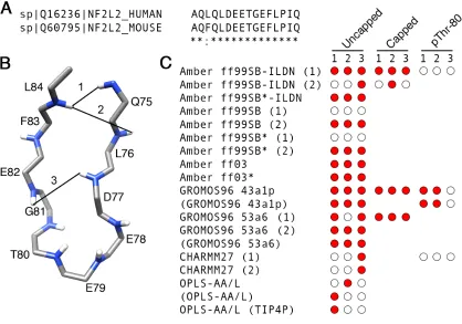
Figure 2.4 Nrf2 β-hairpin sequence alignment and native contacts.
0.1 µs of the simulations between hydrogen atom pairs matching those observed by Tong et al. (30) were considered to be native contacts.
We compared the NMR-derived cross-strand 1H, 1H NOEs determined by (30) to the corresponding time-averaged distances from our MD simulations. Time-averaged distances < 6 Å between hydrogen atom pairs matching those observed in (30) were considered to be native contacts. Because the united-atom GROMOS96 force fields used in this study do not explicitly represent every hydrogen atom, we restricted our analysis to backbone amide hydrogens, which were explicitly represented in all force fields. NOEs between adjacent residues and those involving F74, were excluded from the analysis. This reduced the number of experimentally determined native contacts used in this analysis to three (Q75 HN:L84 HN, L76 HN:L84 HN and D77 HN:E82 HN). They are depicted in Figure 2.4B.
The presence or absence of each of the three contacts is shown in Figure 2.4C. For the uncapped peptides, the Amber ff99SB-ILDN (1), Amber ff99SB*-ILDN, Amber ff99SB (2), Amber ff99SB* (2), Amber ff03, Amber ff03*, GROMOS96 43a1p and GROMOS96 53a6 simulations, including those which used charge-groups, had at least 2 of the 3 native contacts (Figure 2.4C). Once again, there were differences between the Amber replicas (Figure 2.4C). Notably, in the Amber ff99SB-ILDN (2), Amber ff99SB (1) and Amber ff99SB* (1) simulations, only one or none of the native contacts were present, while their replicas had all three (Figure 2.4C). The CHARMM27 and OPLS-AA/L simulations had only 1 out of the 3 native contacts (Figure 2.4C). The capped peptides were able to form all 3 native contacts, but differences between duplicates were also evident. The Amber ff99SB-ILDN (1) simulation had all 3 contacts while its
duplicate had only 1 (Figure 2.4C). Native contacts were reduced in all pThr-80 simulations compared to their unphosphorylated counterparts (Figure 2.4C).