ISSN 2286-4822 www.euacademic.org
Impact Factor: 3.1 (UIF) DRJI Value: 5.9 (B+)
A Study on Morphometric Characteristics of
Sonitpur District, Assam
DR. PRASENJIT DAS Assistant Professor Department of Geography Bajali College, Pathsala, Assam India
Abstract:
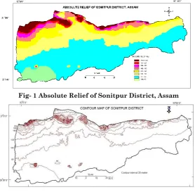
An attempt has been made for morphometric study on Sonitpur District of Assam. Absolute Relief (AR), Relative Relief (RR), Dissection Index (DI), Average Slope (AS) and Stream Frequency (Fu) are the different geomorphic parameters which have been analysed in the study area for morphometric analysis and to prepare the various thematic maps. These parameters have been analysed from SOI toposheets. The entire study area has been divided into 1331 grids of four sq. km each and all parameters are calculated for each grid. From the morphometric study of the study area, it is found that northern part is hilly (highest elevation 456 meters); middle and southern part is almost plain although three isolated hillocks are present in the southern parts which are made up of archean gneisses with a height varying from 80 to 172m above the mean sea level.
Key words: Morphometric study, Absolute relief, Average slope, Dissection index, Stream Frequency
Introduction
unites the qualities of homogeneous and continuous relief due to the action of common geological and geomorphological processes. Analysis of morphometric characteristics is a fundamental requirement of landform study of any area. Morphometry is defined as the measurement and mathematical analysis of the configuration of the earth’s surface and of the shape and dimension of its landforms (Clarke, 1966). Morphometric methods though simple, have been applied for the analysis of area-height relationships, determination of erosion surfaces, slopes, relative relief and terrain characteristics as a whole. The morphometric analysis of different regions had been done by various scientists using conventional methods (Horton, 1945; Smith, 1950; Strahler, 1956). In the present study morphometric analyses of Sonitpur District have been carried out with a view to understand the geomorphic characteristics of the study area.
The Study Area
Sonitpur district is situated in the north-bank plain of the state of Assam. The district is sandwiched by the Brahmaputra River to the south and the Himalayan foothills of Arunachal Pradesh to its north. The area is characterized by lowlands with elevation varying between 10-80 meters, 80-100 and 100-200 meters (Saikia et al, 2008). A small strip of low hills on its northern limits with elevation ranging from 200 to 456 meter exists on its north western margin. Several rivers flowing parallel to one another in a north-south trend dissect the district as they flow down the foothills to the Brahmaputra
River. The total area of the Sonitpur District is 5324 km2 and is
there is a marked variation within the district. Rainfall is quite high at 1384 mm (GoA, 2004). According to Champion and Seth (1968), the forests in the study area are comprised primarily of subtropical evergreen, tropical semi-evergreen, tropical moist deciduous and riverain forest/grasslands.
Database and Methodology
For the preparation of base map and for morphometric analysis of the study area, topographical sheets of 1:50,000 scale of the Survey of India are used.
Absolute Relief (AR), Relative Relief (RR), Dissection Index (DI), Average Slope (AS) and Stream Frequency (Fu) are the different geomorphic parameters which have been analysed in the study area to differentiate physiographic characteristics and to prepare the various thematic maps. The entire study area has been divided into 1331 grids of four sq. km each and all parameters were derived and calculated for each grid.
Absolute relief gives the elevation of any area above the sea-level Absolute elevation in each grid has been computed from spot heights, triangulation points wherever available and from the maximum contour value passing through the grids (with contour interval 20m).
Relative relief represents the difference in elevation between the highest and lowest points falling in a unit area. For the purpose of relative relief analysis, the height difference between the highest and lowest elevation within each grid is
computed with a contour interval of 20m.
and relief energy of the area. It has been calculated by the following methodology:
Relative Relief (R.R.) Dissection Index (D.I.) = __________________
Absolute Relief (A.R.)
The term ‘slope’ in its broadest sense means an element of earth’s solid surface, including both terrestrial and submarine surfaces; it is, therefore, simply an element of the interface between the lithosphere or atmosphere (Strahler, 1956). Slope refers to the angle which any part of the earth’s surface makes with horizontal. It is an element of the interface between lithosphere and either hydrosphere or atmosphere (Fairbridge 1968).
Computation of slope angles from topographical maps or through field measurement involves tedious and time-consuming procedures. Several techniques of the derivation and computation of average slopes from topographical maps have been suggested from time to time e.g. Smith (1935), but the technique of Wentworth, being easier and involving lesser measurement and calculation and more rapid procedure than other schemes, has been adopted for the slope analysis in the area.
The formula devised by Wentworth is given below:
Average Slope = Tan Ө = N X CI/3361
Where, N = Average no. of contour crossing in an area per sq. mile. CI = Contour interval in feet
3,361 = A constant figure
capacity of the soil. It is an index of the various stages in landscape evolution.
Horton (1932, 1945) introduced stream frequency as the number of stream segments per unit area.
Numerically, it is defined by the relation
Fu = (N) u/Au Where
Fu = Stream frequency in no/km2
(N) u = Sum of total number of stream segments of all orders Au = Total area of the drainage basin in sq. km
The expression Fu gives the average frequency of streams in the basin.
The various geomorphic attributes of the study area are discussed below.
Absolute Relief (AR)
Table-1 Distribution of Absolute Relief A bso lut e R eli ef C ate go rie s( m ) Grid F re que n cy
Grid Fre
que nc y (%) A re a (sq . k m ) C um ula tiv e A re a A re a (%) C um ula tiv e A re a (%) Major Absolute Relief Groups
Above 180 61 4.58 244 4.58 4.58 4.58 Above 160m – Very High 312 sq. km (5.86%)
160-180 17 1.28 68 312 1.28 5.85
140-160 31 2.33 124 436 2.33 8.18 120-160m High
412 sq. km (7.74%)
120-140 72 5.41 288 724 5.41 13.59
100-120 158 11.87 632 1356 11.87 25.46 80-120m High Moderate 1980 sq. km (37.19%) 80-100 337 25.32 1348 2704 25.32 50.78
60-80 424 31.84 1696 4400 31.84 82.63 Below 80m Low 2620 sq. km (49.21%) Below 60 231 17.37 924 5324 17.37 100.00
1331 100 5324 5324 100 100
Distributional Pattern of Absolute Relief
The different Absolute Relief categories reveal a peaked grid frequency distribution between below 80m and 80-100m categories.
Table-1 Reveals that very high and high relief categories have insignificant spatial distribution (5.86%, and 7.74% respectively). On the other hand large part of the study area has moderate to low absolute relief groups (37.19% and 49.21% respectively). The distribution of these groups is discussed below.
Very High Absolute Relief (Above 160m)
High Absolute Relief (120 To 160m)
The terrain representing the high absolute relief is located to the south of the very high absolute relief. This part is also densely forested but recently lot of deforestation has taken place and the forest area is taken over by human settlements.
Fig- 1 Absolute Relief of Sonitpur District, Assam
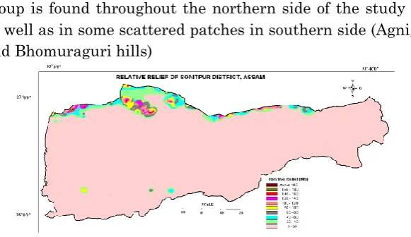
Fig. 2 Contour Map of Sonitpur District
Moderate Absolute Relief (80 To 120m)
The terrain representing the moderate absolute is located to the south of the high absolute relief. Here both forest and human settlements are found with the dominance of the later.
Low Absolute Relief (Below 80m)
is prone to flood which often creates havoc damaging both life and property of the people.
Relative Relief (RR)
For the purpose of relative relief analysis, the height difference between the highest and lowest elevation within each grid is computed with a contour interval of 20 m. The relative relief varies from 0m in the south to 150m in the north and northeast. The grid values are classified into eight categories (Table- 2). With a class interval of 20m, ranging from less than 20m to more than 140m above mean sea level. The spatial distribution of these categories is shown in fig-3.The different relative relief categories reveal a decrease above 20-40m category which indicates an almost plain relief of the study area. For qualitative assessment these categories have been classed into four major groups (Table-2) and discussed below.
Table 2 Distribution of Relative Relief in Sonitpur District
R ela tive R eli ef C ate go ry
Grid Fre
que
nc
y
Grid Fre
que
nc
y
(%) Are
a (S q. K m ) C um ula tiv e A re a (S q. k m ) A re a
(%) Cum
ula tiv e A re a( %) (%)
Major Relief Groups
Above 140
3 0.22 12 12 0.22 0.22 Above 120m
Very High 32 sq. km (0.60%)
120-140 5 0.38 20 32 0.38 0.60
100-120 6 0.45 24 56 0.45 1.05 80-120m High
68 sq. km (1.27%)
80-100 11 0.83 44 100 0.83 1.88
60-80 14 1.05 56 156 1.05 2.93 40-80m Moderate
128sq. km (2.40%)
40-60 18 1.35 72 228 1.35 4.28
20-40 32 2.40 128 356 2.40 6.68 0-40m Low
5096 sq. km (95.72 %)
0-20 1242 93.32 4968 5324 93.32 100
Distributional Pattern of Relative Relief
A perusal of Table-2 reveals that low relief (95.72%) dominates the entire study area, moderate relief (2.40%) comes in distant second. High and very high reliefs (1.27% and 0.60%) occupy only a very insignificant portion of the study area.
Very High Relative Relief (Above 120m)
It covers a negligible area (0.60% or 32 sq. km) in the study area and is found over north and northwestern side of the study area. In these areas river valleys and hills exist together resulting in such high relative relief.
High Relative Relief (80-120m)
It covers an insignificant area (1.27% or 68sq. km) and is spread over as clusters in the northeastern, northern and northwestern side of the study area. The upper reaches of Jia Bharali and Gabharu River have high relative relief.
Moderate Relative Relief (40-80m)
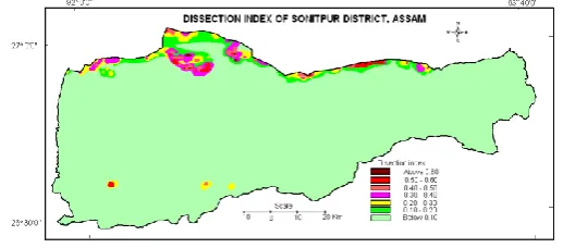
This group covers 2.40% or 128sq.km of the study area. This group is found throughout the northern side of the study area as well as in some scattered patches in southern side (Agnigarh and Bhomuraguri hills)
Fig 3 Relative Relief of Sonitpur District
Low Relative Relief (0-40m)
plain area and that is why more than 95 percent of the study area has low relative relief.
Dissection Index
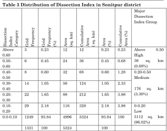
In the study area, dissection index is computed for 1331 grids. The value varies from 0.0 to 0.64 and it has been classified into seven categories (Table-3) with a class interval of 0.10, ranging from less than 0.10 to above 0.60. The spatial distribution of these categories is shown in Fig.-4. For qualitative assessment, these seven categories have been classed into three groups.
Fig. 4 Dissection Index of Sonitpur District
Distributional Pattern of Dissection Index
A perusal of Table 3 reveals that maximum grid frequency lies under the low groups covering 96.02% of the total frequency. It indicates plain nature of the topography in the study region. The different dissection index groups are discussed below.
Very High (Above 0.50)
Table 3 Distribution of Dissection Index in Sonitpur district Di sse ctio n Ind ex C ate go ry Grid F re que nc y
Grid Fre
que
nc
y
(%) Are
a (sq . k m ) C um ula tiv e A re a ( sq . k m ) A re a
(%) Cum
ula tiv e A re a (%) Major Dissection Index Group Above 0.60
3 0.23 12 12 0.23 0.23 Above 0.50 High
36 sq. km (0.68%)
0.50-0.60
6 0.45 24 36 0.45 0.68
0.40-0.50
8 0.60 32 68 0.60 1.28 0.20-0.50 Medium
176 sq. km (3.30%)
0.30-0.40
14 1.05 56 124 1.05 2.33
0.20-0.30
22 1.65 88 212 1.65 3.98
0.10-0.20
29 2.18 116 328 2.18 3.98 0-0.20 Low
5112 sq. km (96.02%) 0.0-0.10 1249 93.84 4996 5324 93.84 100
1331 100 5324 100
Moderate (0.20-0.50)
This group is also found in the northern part of the study area and it also covers a negligible area (3.30%). Three patches of moderate dissection are also found in the southern part of the study area where some small hillocks are found.
Low (0.0-0.20)
This group dominates the entire study area as it occupies 96.02% of the total area.
Average Slope (As)
The term ‘slope’ in its broadest sense means an element of earth’s solid surface, including both terrestrial and submarine surfaces; it is, therefore, simply an element of the interface between the lithosphere or atmosphere (Strahler, 1956).
km. i.e. per grid is counted ( contour crossing per side of the grid divided by four = contour crossing per grid). With the Wentworth’s formula, average slope per grid is computed (the value obtained by the formula is converted into degrees). These average slope values obtained have been classified into 6 categories (Table-4) with an interval of 2.5. For qualitative assessment, these six categories have been classed into three groups. The spatial distribution of these categories is shown in Fig-5. The slope within the study area varies from 0° in the south to 14° as isolated patch in the northwestern part of the study area.
Fig. 5 Average Slope Map of Sonitpur District
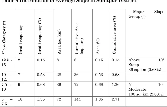
Table 4 Distribution of Average Slope in Sonitpur District
S lo pe C ate go ry ( °) Grid F re que n cy Grid F re que n cy ( %) A re a (sq . k m ) C um ula tiv e A re a (sq . k m ) A re a (%) C um ula tiv e ar ea ( %)
Major Slope Group (°)
12.5 -
15 2 0.15 8 8 0.15 0.15 Above Steep 10°
36 sq. km (0.68%) 10 –
12. 7 0.53 28 36 0.53 0.68
7.5 –
10 9 0.68 36 72 0.68 1.36 5° Moderate - 10° 108 sq. km (2.03%)
2.5 – 5
31 2.33 124 268 2.33 5.04 0° - 5°
Gentle
5180 sq. km (97.29%)
0 – 2.5
1264 94.96 5056 5324 94.96 100
1331 100 5324 5324 100
Distributional Pattern of Slope
The different slope categories show that maximum portion of the study area has gentle slope (97.29%). Since the study area is essentially a part of Brahmaputra valley, which is almost totally a plain area except some monadnock like features here and there, maximum portion of the study area has gentle slope. A perusal of table-4 reveals that steep slope group has negligible areal extent (0.68%). Similarly moderate slope group only occupies 2.03% of the total study area. The distribution of various slope categories is discussed below.
Steep Slope (Above 10°)
Steep slope covers about 36 sq. km or 0.68 per cent of the study area. This category occurs in the northern side of the study area which is hilly in character. This category is also found in the southern part of the study area where it occurs as isolated patches where monadnocks like features are found.
Moderate Slope (5°-10°)
This category covers 108 sq. km or 2.03% of the study area. This category is also mainly found in the northern part which is hilly in character.
Gentle Slope (0°- 5°)
Stream Frequency (Fu)
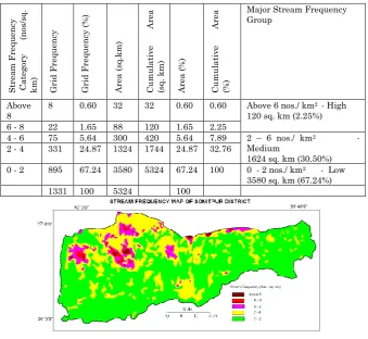
The stream frequency within the study area varies from 0 nos. in the southernmost part to 10nos. scattered towards the northern and eastern part of the study area. The grid wise computed drainage frequencies are classified into five categories (Table-5) with a class interval of 2, ranging from below 2 nos. per sq. km to above 8 nos. per sq. km. The spatial distribution of these categories is shown in Fig.-6. These categories have been classed into three major stream frequency groups and discussed in table-5.
Table 5 Distribution of Stream Frequency in Sonitpur District
Fig.6 Distribution of Stream Frequency of Sonitpur District
S tre am F re qu enc y C ate go ry (n os/ sq . k m ) Grid F re que n cy Grid F re que n cy ( %) A re a (sq .k m ) C um ula tiv e A re a (sq . k m ) A re a (%) C um ula tiv e A re a (%)
Major Stream Frequency Group
Above
8 8 0.60 32 32 0.60 0.60 Above 6 nos./ km
2 - High 120 sq. km (2.25%) 6 - 8 22 1.65 88 120 1.65 2.25
4 - 6 75 5.64 300 420 5.64 7.89 2 – 6 nos./ km2 - Medium
1624 sq. km (30.50%) 2 - 4 331 24.87 1324 1744 24.87 32.76
0 - 2 895 67.24 3580 5324 67.24 100 0 - 2 nos./ km2 - Low 3580 sq. km (67.24%)
Distribution of Stream Frequency in Sonitpur District
The different drainage frequency categories reveal a peaked grid frequency distribution between 0-2 nos. per sq. km and 2-4 nos. per sq. km stream frequencies. A perusal of (Table-5) indicates that high stream frequency group has insignificant distribution of 2.25% in the study area. The distribution of various stream frequency groups are discussed below.
High Stream Frequency (Above 6 Nos/ Km2)
It is scattered mainly in the northern and eastern part of the study area in discrete patches.
Moderate Stream Frequency (2- 6 Nos/ Km2)
This group occurs as large patches all over the region especially in the northern and eastern part. The spatial distribution of this group does not indicate any influence of lithology or structure.
Low Stream Frequency (Below 2 Nos/ Km2)
This is the dominant stream frequency group in the study region as it covers 67.24 % of the study area. Except the northernmost part, where it is almost absent, this group dominates everywhere in the study area.
Conclusion
found that that very high and high relief categories have insignificant spatial distribution (5.86%, and 7.74% respectively). On the other hand large part of the study area has moderate to low Absolute Relief groups (37.19% and 49.21% respectively). From the study of Relative Relief, it is found that the relative relief varies from 0 m in the south to 150m in the north and northeast. Low relief (95.72%) dominates the entire study area; moderate relief (2.40%) comes in distant second. High and very high relief (1.27% and 0.60%) occupies only a very insignificant portion of the study area. From the study of Dissection Index, it is found that dissection index value varies from 0.0 to 0.64. and maximum grid frequency lie under the low groups covering 96.02% of the total frequency which indicates plain nature of the topography in the study region. From the study of Average Slope, it is found that the slope within the study area varies from 0° in the south to 14° as isolated patch in the northwestern part of the study area. The different slope categories show that maximum portion of the study area has gentle slope (97.29%). Since the study area is essentially a part of Brahmaputra valley, which is almost totally a plain area except some monadnock like features here and there, maximum portion of the study area has gentle slope. From the study of stream frequency, it is found that the stream frequency within the study area varies from 0 nos. in the southernmost part to 10nos. scattered towards the northern and eastern part of the study area. The different stream frequency categories reveal a peaked grid frequency distribution between 0-2 nos. per sq. km and 2-4 nos. per sq. km stream frequencies. Further it is found that high stream frequency group has insignificant distribution of 2.25% in the study area.
REFERENCES
Champion, H. G. and Seth, S. K. 1968. A Revised Survey of the
Forest Types of India. New Delhi: Government of India
Clarke, J.I. 1966. “Morphometry from maps.” In Essays in
Geomorphology, edited by G.H. Dury, 235-274. American
Elsevier Publication. New York.
Crevennaa, A. B., Rodrı́guez, V.T., Sorani, V., Frame, D. and Ortiz, M.A. 2005. “Geomorphometric Analysis for Characterizing Landforms in Morelos State, Mexico.”
Geomorphology 67: 407–422.
Fairbridge, R.W. 1968. “The encyclopedia of geomorphology.” In
Encyclopedia of Earth-Science Series, V.III. New York:
Reinhold Book Corp., 1295.
GoA. 2004. Statistical Handbook of Assam. Directorate of
Economics and Statistics, Govt. of Assam.
Horton, R.E. 1932. “Drainage basin characteristics”. Trans. Am.
Geophysical Union 13: 350-361.
Horton, R.E. 1945. “Erosional development of streams and their drainage basins, hydrophysical approach to quantitative
morphology.” Bull. Geol. Soc. Am. 56: 275-370.
Nir, D. 1957. “The Ratio of Relative and Absolute Altitude of
Mt. Carmel.” Geographical Review 27: 564-569.
Saikia, A., Hazarika, R., Sahariah, D., Barman, E., and Pio, S. 2008. “No Living Space? Shrinking Habitat and Human Elephant Conflict in Assam, India.” Final Report submitted to Rufford Small Grants foundation.
Smith, G.H. 1935. “The relative relief of Ohio.” Geog. Rev. 25:
272-284.
Strahler, A. N. 1956. “Quantitative slope analysis.” Bull. Geol.