Comparison of Position Control of Ball and
Beam System using Phase lead and PID
Controller
Sameera.R1, Arun.S.Mathew2
PG Student [CS], Dept. of EEE, Mar Baselios College of Engineering and Technology, Trivandrum, Kerala, India1 Assistant Professor, Dept. of EEE, Mar Baselios College of Engineering and Technology, Trivandrum, Kerala, India2
ABSTRACT:The ball and beam system is the classical mechanical system having unstable dynamics and strong nonlinear characteristics which makes the control a challenging task. The control problem is difficult as the ball position changes continuously with the beam angle. In this paper a Phase lead controller and Computational Optimization based PID controller is used to enhance a better position control. The controllers are designed based on some design criteria. The simulations of the proposed controllers are analyzed using MATLAB Simulink and the performances of the system using both the controllers are compared and the response is analyzed. The results show that the PID tuned using Computational optimization shows satisfactory response compared to the phase lead controller. KEYWORDS:nonlinear, position control, phase lead, computational optimization.
I.INTRODUCTION
The Ball and Beam system is one of the widely used and important laboratory models for control system techniques. Nonlinearities and instabilities are considered to be a major challenge for control systems. The ball and beam system is such a system having nonlinearities and instabilities. The ball and beam is an open loop unstable system that is the ball will continuously roll on beam until a controller is used. Different control strategies can be used to control the ball position. It is generally linked to real time control problems such as control of aircraft during landing. There is a high risk of aircraft tumbling without a controller. Learning the dynamics and control of ball and beam system helps to solve such problems. The objective is to control the ball position to a predefined position. The feedback information of the ball position can be used as the control signal. The control voltage signal operates the DC motor and the torque generated drives the beam to a desired angle.
II.DYNAMICS OF BALL AND BEAM SYSTEM
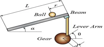
The physical setup of ball and beam is shown in Fig 1.A metal ball is placed on the beam where it is allowed to roll along the beam. One end of the beam is attached with a lever arm and the other end is attached with a servo gear. When the servo gear turns by an angle
the beam angle get changed by the lever by
.This causes movement of the beam which forces the ball to roll as the acceleration is directly proportional to the tilt of beam angle. A linear transducer is fitted along the beam to measure the ball position. The ball and beam system is open loop unstable system because the ball position increases without limit for a fixed beam angle. So balance control is considered to be a difficult control problem for ball and beam system. Hence a suitable controller is necessary to be designed for the system.Fig 1: Schematic diagram of Ball and beam system
L
- length of the beamd
- Distance between centre of the gear and the joint between the gear armsr
- Ball position
- Beam angle
- Rotation angle of gearThe modeling of Ball and beam system helps to understand the complete dynamics of the system. Lagrange approach is used for the modeling of ball and beam system. It is based on energy balance of the system. Assume that the ball rolls without slipping The parameters to develop the dynamics of the system is shown in Table 1.
Table 1: PARAMETERS OF BALL AND BEAM SYSTEM
SL NO
PARAMETERS VALUE
1 Mass of ball 0.064kg 2 Radius of ball 0.0127m 3 Beam length 0.4255m 4 Distance between servo gear shaft and coupled joint 0.0254 m 5 Acceleration due to gravity -9.8m/s2
The Euler-Lagrange is used to define the kinetic and potential energy for the system is shown in equations (1) and (2).
(1)
2 2
2
5 7 2
1
x m x
m J
b
J
-Moment of inertia of beamb
m
- Mass of the ballx
- Position of the ball
- Beam angleg
-acceleration due to gravityThe Lagrange function is the difference between kinetic energy and potential energy of the system.
(3) Lagrange equations are obtained as follows.
L L dt d (4) 0 x L x L dt d (5)
Where
x
-ball position on beam
- beam angle(6)
(7)
Linearizing equation (7) around the operating points, the equation becomes as follows. (8)
The beam angle and the angle of the gear can be related by equating the arc distance is specified as follows
beam armL
r
(9)On substituting equation (9) in (8) and taking Laplace transforms, the transfer function of the ball and beam transfer function with system parameters can be represented as
(10)
The ball and beam system is an inherent open loop unstable system. The open loop step response is shown in Fig 2.The
response shows that the system is unstable. So some controllers are required to bring the system to a stable one.
V
T
L
cos 2 2 gx m x x m x m
Jb b b b
0 sin 7 5 2 x g x sin 7 5 g x
2Fig 2 : Open loop response of ball and beam system
III.DESIGN OF PHASE LEAD CONTROLLER
The lead controllers are extensively used which can increase the stability and speed of response of the system. This controller is designed by determining
from the amount of phase needed to satisfy the required phase margin and determine T to place the added phase at new gain crossover frequency.The design criteria for ball and beam system a. Settling time should be less than 3.5 sec b. Overshoot should be less than 10%
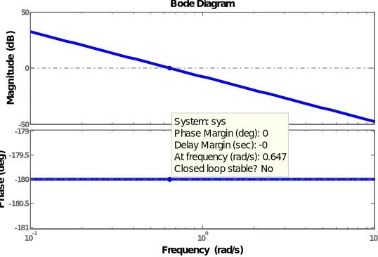
The open loop transfer function of ball and beam system is shown in equation (10) and bode plot of open loop response is shown in Fig 3
Fig 3: Bode plot of open loop system
From the plot, we obtain the phase margin as zero. This clearly indicates that the open loop system is unstable. Increase the phase margin in order to obtain a stable system response .Phase lead controller is such a compensator controller
-50 0 50
M
a
g
n
it
u
d
e
(
d
B
)
Bode Diagram
Frequency (rad/s)
10-1 100 101
-181 -180.5 -180 -179.5 -179
System: sys Phase Margin (deg): 0 Delay Margin (sec): -0 At frequency (rad/s): 0.647 Closed loop stable? No
P
h
a
s
e
(
d
e
g
A first order phase lead controller can be represented by
T s
T s K s C
1
1 (11)
Where T > 0 and
1
Ts
Ts
K
s
C
1
1
(12)
T
/
1
and 1/T are the corner frequencies. The maximum added phase for phase lead compensator is 90 degree. The lead compensator helps to improves the speed of response and reduces the overshoot. This improves the transient response of the system.2 1
e
M
P (13)
corresponds to 10% peak overshoot is 0.591.Generally
*
100
will give the minimum phase margin needed to obtain the desired overshoot. Therefore we require a phase margin of59
.
1
60
0A. Design steps for obtaining T and
a. Find the positive phase needed.
Here we need at least 60 degree for the controller. b. Find the center frequency
The relation between bandwidth frequency and settling time gives 1.66 rad/s. Therefore we want a centre frequency just before this. Choose 1
c. Obtain the value of
sin
1
sin
1
For
60
0
.
0718
d. Find T and
T
from the given equationsa
w
T
1
w
a
T
Substituting these values
T
0
.
1614
and732
.
3
T
Fig 4: Bode plot of phase lead controller to the system
From the plot it is clear that the phase margin now obtained is near to 60 degree and the closed loop is stable. The transfer function of phase lead controller obtained is
s
s
s
C
1614
.
0
1
73
.
3
1
5
(14)IV.DESIGN OF PID CONTROLLER
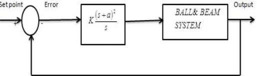
PID controllers are widely used in the industry due to its simple structure and robust control. PID controller helps to acquire the most optimum results. The major task of PID controller design is to obtain the controller parameters for achieving desired response. There are many tuning rules available for unstable and integrating systems but only a few tuning methods for double integrating system. So it is essential to develop new control strategies for double integrating system for attaining good response. Here Computational Optimization approach is used to obtain an optimal set of PID values. The PID controller is given by
s
a
s
K
s
C
2
(15)PID controller with computational optimization approach for ball and beam system is shown in fig 5.
Fig 5: Block diagram for PID controller using computational optimization
-100 -50 0 50 100
M
a
g
n
it
u
d
e
(
d
B
)
Bode Diagram
Frequency (rad/s)
10-2 10-1 100 101 102
-180 -150 -120
System: untitled1 Phase Margin (deg): 59.3 Delay Margin (sec): 0.81 At frequency (rad/s): 1.28 Closed loop stable? Yes
P
h
a
s
e
(
d
e
g
parameter values are obtained using MATLAB code. Assume the region of search for ‘K’ and ‘a’.We have to expand it, if the solution does not exist in this region Select the step size for ‘K’ and ‘a’. The step size should be small in orderto avoid large number of computations. Here the step size chosen is 0.2 for ‘K’ and 0.1 for ‘a’. The MATLAB code should be written such that the nested loops in the code first compute for the lowest values and then computes for the highest. We select those values of ‘K’ and ‘a’ that gives the smallest overshoot and better settling time.
The values obtained are
K=15, a=0.4. The transfer function of the controller is given by
s
s
s
C
2
)
4
.
0
(
15
(16)
s
s
s
s
C
15
12
2
.
4
2
(17) The transfer function of the PID controller is given by
s
K
s
K
s
K
s
C
d
p
i2
(18) The PID parameters obtained are
15
4
.
2
12
i dp
K
K
K
V. SIMULATION RESULTS
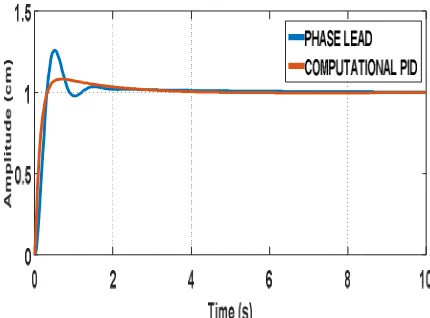
Fig 6 shows the step response of phase lead controller and PID controller implemented in the ball and beam system.Table 2 shows the performance of step response of Phase Lead controller and computational Optimization PID controller implemented in the Ball and Beam system
Table 2: COMPARISON OF PHASE LEAD AND PID CONTROLLER
CONTROL TECHNIQUE
MAXIMUM OVERSHOOT
(%)
SETTLING TIME
(s)
PHASE LEAD 26.1 1.92 COMPUTATIONAL PID 8.03 2.1
It is clear that PID tuned by Computational Optimization satisfies the design criteria that is maximum overshoot is less than 10% and settling time is less than 3.5 s. It shows better response than Phase lead controller.
VI.CONCLUSION
The ball and beam system have been widely used for studying new control techniques. Phase lead controller and Computational Optimization based PID controller is used for the analysis of Ball and Beam System. The proposed controllers are analyzed using MATLAB SIMULINK platform. Simulation results show that the Computational Optimization based PID controller satisfies the design criteria and can perform well for controlling the ball position. The Computational Optimization approach can be applied to any double integrating unstable system in order to obtain better closed loop system performance.
REFERENCES
[1] J.Hauser,S.Sastry and P.Kokotovic ,Nonlinear control via approximate input-output linearization :ball and beam example,IEEE Transactions on Automatic Control,Vol.37,No.3,392-398,March1992.
[2] P.H.Eaton,D.V.Prokhorov,”Neurocontroller Alternatives for fuzzy ball and beam systems with non uniformnon linearfriction”,IEEE Transactions On Neural Networks,Vol.11,No.2,March 2000.
[3] R.M.Hirschorn,”Incremental Sliding Mode Control for Ball and Beam”,IEEE Transactions on automatic control,vol.47,no.10,October 2002. [4] Y.T.Hsiao,C.L.Chuang,C.C.Chien ,”Ant Colony Optimization for Designing of PID controllers,”IEEE International Symposium on Computer
Aided Control Systems Design, September 2004.
[5] J .S.Kim,G.M.Park and H.L.Choi,”Sliding mode control design under partial state feedback for ball and beam systems,”International Conference on control, Automation and Systems,Gyeonggi-do,Korea,2010.
[6] M.Keshmiri,A F Jahromi,A F Mohebbi,M H Amoozgar and W.F Xie,”Modeling and Control of ball and beam system using model based and non model based control approaches, “International Journal on smart sensing and intelligent systems,vol.5,no.1,March 2012
[7] D.Puangdownreong and A.Sakulin,”Obtaining an optimum PID controller for unstable systems using current search”, International Journal of Systems Applications, Engineering and Development,vol.6,2012.
[8] Y.H.Wang,W.S.Chan and C.W.Chang,”T-S Fuzzy Model based Adaptive Dynamic Surface Control for Ball and Beam”,IEEE Trans.Ind.Electron”,vol.60.no.6,June 2013.