A Large and Quick Induction Field Scanner for Examining
the Interior of Extended Objects or Humans
Martin Klein and Dirk Rueter*
Abstract—This study describes the techniques and signal properties of a powerful and linear-scanning 1.5 MHz induction field scanner. The mechanical system is capable of quickly reading the volume of relatively large objects, e.g., a test person. The general approach mirrors magnetic induction tomography (MIT), but the details differ considerably from currently described MIT systems: the setup is larger and asymmetrical and it operates in gradiometric modalities, either with coaxial excitation with destructive interference or with a single excitation loop and tilted receivers. Following this approach, the primary signals were almost completely nulled and test objects’ real or imaginary imprint was obtained directly. The coaxial gradiometer appeared advantageous: exposure to strong fields was reduced due to destructive interference. Meanwhile, the signals included enhanced components at higher spatial frequencies, thereby obtaining a gradually improved capability for localization. For robust signals the excitation field can be powered toward the rated limits of human exposure to time varying magnetic fields. Repeated measurements assessed the important signal integrity, which is affected by the scanner’s imperfections, particularly any motions or respiratory changes in living beings during or between repeated scans. The currently achieved and overall figure of merit for artifacts was 58 dB for inanimate test objects and 44 dB for a test person. Both numbers should be understood as worst case levels: a repeated scan with intermediate breathing and drift/dislocations requires 50 seconds whereas a single measurement (with respiratory arrest) only takes approximately 5 seconds.
1. INTRODUCTION
1.1. General Background
Magnetic induction fields permeate the free space and volume of low conducting materials, thereby allowing the non-contacting localization of features inside an opaque test object. Magnetic induction tomography (MIT) images the conductivity variation inside a test volume [1, 2]. The exciting induction fields are perturbed somewhat by the object’s internal eddy currents and then picked up by several sensor coils. The sensor signals then are computed extensively, concluding in a tomographic image. Attractive features of MIT include the non-contacting modality and the relative harmless fields. On the other hand, MIT provides only rather blurred images despite considerable progress over the past decade. In addition, it remains difficult to gain a pattern reconstruction from the received signals.
Various applications [1] of MIT have been proposed for metallic samples and for low-conductivity objects, including biomedical imaging [2–5]. Although it sounds attractive, biomedical MIT remains challenging due to the nature of induction fields and the conditions of living beings. The three-dimensional (3D) distribution of low-conducting materials inside human beings, even with low contrast between different compartments (organs), causes a multitude of problems. A further difficulty appears in motion or displacement artifacts, which can easily corrupt the delicate image reconstruction of MIT [4, 6].
Received 7 August 2017, Accepted 7 October 2017, Scheduled 20 October 2017
* Corresponding author: Dirk Rueter ([email protected]).
The most frequently described MIT systems consist of a circular [7–9] or hemispherical [5] arrangement of multiple transmitter and receiver coils placed around the measurement volume. The setup is often surrounded by a metallic shield to protect the delicate signals from incident electromagnetic interference (EMI) from the environment. The circular symmetry appears reasonable to approach a test object equally from all sides. For this geometry, there are two-dimensional (2D) and 3D image reconstructions [e.g., [1–12], even for low-conductivity objects [3, 13]. Similar to magnetic resonance imaging (MRI), an MIT tube should be as narrow as possible with respect to the test object to best utilize the available measurement volume.
Circular MIT faces a geometrical disadvantage in that the test object must fit into/through a narrow tube. Clearly, it is not the most comfortable procedure when it comes to requiring a person to remain motionless during a prolonged measurement cycle inside a narrow MRI tube. A more convenient and quicker measurement for humans ultimately would allow for new applications, such as security. Modern airport scanners for mass processing cannot detect non-metallic and dangerous materials inside the body. Quick measurement would also be more desirable for less pronounced motion artifacts.
One study recently outlined a planar MIT system (PMIT) with fewer geometrical restrictions [14]. The PMIT can approach much larger relative objects from only one side, thereby leaving the test object in its natural arrangement or posture. The described PMIT consisted of a planar array of 4×4 coils on an 18×18 cm2 board and was capable of 3D near-subsurface imaging of metallic objects. Due to the limited range of the induction fields, both for emission and detection, the system obtained an imaging depth of slightly more than 5 cm. Although it might be advantageous to apply such a system to potentially large objects, this advantage was diminished by the PMIT’s limited detection depth, a limitation resulting primarily from excitation and sensing from only one side, i.e., in reflection geometry. The previous PMIT study [14] relates somewhat to the presented scanner in this paper. Our technique differs, however, in that it operates in transmission geometry (i.e., using a through-shining excitation field from the opposing side), thereby providing a better sense of depth. Furthermore, it not only provides a single measurement value for each transmitter-detector pair, but characteristic signal traces with many more and independent measurements from each sensor due to a controlled and linear motion of the test object. This feature allows for a larger amount of useful data, and the signal traces permit mathematical operations like a Fourier transformation. A recent study showed that a circular MIT [15] with eight coils provided an increased amount of independent measurement data due to an additional and controlled rotation of the test object, which can improve the imaging capability considerably. Without rotation and the eight coils, only 7 + 6 + 5 + 4 + 3 + 2 + 1 = 28 independent measurement values [15] were available from the test object. Limited data from the measurement volume reduce the imaging capability and resolution.
1.2. Outline of the Scanner and Objective
This technically-oriented work investigates a quick and convenient application of an induction field scanner to large objects and/or humans. In addition to the generally large dimensions (Fig. 1) with respect to previously described MIT systems [1], further differences include powerful excitation, distinct asymmetry, strict separation between excitation and sensors, and near-perfect gradiometry. It uses merely a single excitation source and potentially many smaller receiver coils at suitable positions.
As Fig. 1 shows, for the technical evaluation of the system, only two sensors (Fig. 1) were installed preliminarily at the height (y-direction) of the excitation axis. A depth determination in simple test objects was possible with the two sensors and their different projections, or “viewing angles”. The setup in Fig. 1 is preliminarily sufficient for evaluating the technical feasibility and available signal quality from such a scanner. More sensors with other projections and different y-position — essential for 3D information and a better resolution — shall be added in a more mature model.
(a) (b)
Figure 1. (a) The scanner uses only one powerful gradiometer for excitation and opposing receivers with different projections. In the current state, only two sensor loops in the x-z plane were applied at the height of the excitation loops (y = 0). More sensors with other projections can be added in the future. (b) Practical setup with an upright test person in the trolley. The upper part of the thorax is at the height of the coil’s axis. For better presentation, a Styrofoam corpus at the left excitation site was removed. This corpus serves as a spacer, ensuring a safe distance from the powerful excitation loops. The trolley, composed almost entirely of dielectric material, travels approximately 2 m over a steel rail.
The presented system is designed to scan a human being in an upright position using a convenient procedure within the rated exposure limits (specific absorption rate, SAR) for induction fields. A person may enter the trolley outside the induction field at x= 0 (currently it is not distinctively strapped or immobilized with suitable support structures, Fig. 1(b)). It then travels through the measurement region and is exposed to stronger fields, typically for less than 5 seconds, before finally leaving the trolley at
x = 210 cm on the other side. Naturally, inanimate test objects (e.g., wood or concrete samples with potential metal inclusions, saline/agar bodies, or metallic patterns for principal investigations) can also be fixed onto the trolley.
A mechanical scan involves additional random vibrations or displacements within the recording run. This condition causes artifacts in the raw signals, which are critical for MIT methods [4, 6], thus raising questions regarding the practical signal integrity. In the currently more common circular MIT systems, the coils are switched electronically, and the total arrangement is virtually motionless. It then provides a quasi-static snapshot, even for a prolonged integration time, and motion artifacts are of no concern for inanimate test objects.
The overall signal integrity is assessable via a characteristic difference between two subsequent scans. In general, a differential measurement in MIT systems can utilize the maximum availablea priori information [16]: only the change of an already well-known (or assumed) test object is noticed in the difference signal. This difference signal indicates the reproducibility and usefulness of the measurement system, and it isolates the signature of a relatively small modification itself.
pronounced during a shorter period of time, and quick procedures are naturally more convenient for test subjects. For most potential patients, it is reasonable to hold on’s breath for a few seconds. A prolonged integration time remains unsuitable and undesirable. For this reason, a rather high — but still permissible — power level here is applied for the exciting induction field, thereby allowing for quick recording.
For practical reasons, a mechanical rotation [15] of the object of interest is not intended here: a rotating person, due to stabilizing reflex movements, presumably causes much stronger motion artifacts. The more general question of why the test object or person here is linearly moved, and the measurement system is held motionless, can be answered as follows: the signals from a moving measurement system and a static object or person would be much more vulnerable to mechanical vibrations or relative dislocations within the measurement system, as variations from the strong primary field rather than the much weaker perturbation would impinge on the signals.
We are currently addressing questions regarding the principal value of such a mechanical scanner as a measurement system. As such, we do not attempt a 3D reconstruction of extended agar models or human beings. Instead, we approach simple 2D presentations and signal differences between two subsequent scans, which are likely more relevant for testing the general performance.
2. METHODS
2.1. Principle Considerations, Formulations and Calculations
The simplest approach for a sensitivity map in MIT is theH·Hmap [17–19]. A sensitivity map describes the measurement signal as a function of an object position inside the measurement volume (forward model). The H·H map can either be experimentally measured (as shown below in the experimental results) or calculated as the scalar product (the inner product or dot product) of the excitation field
H1 and the virtual field H2 of the receiver coil, as described in more detail and demonstrated in [18].
For calculation, the field topologies of the two corresponding coils must be known for every point of the interesting space. This can be approached by, e.g., using analytical expressions for the H field of a current ring (formulation given below). TheH·H map is sufficient for points like high-contrast and isolated test objects or for differential measurements. Other research has shown similar maps quite recently [15]. To determine the validity of the H·H map, the local eddy current circulations around relatively small test objects are required as isolated from the environment. In a practical application,the objects must be sufficiently separated. It is, therefore, well-known that the computer-efficientH·Hmap fails as a forward model for extended and interconnected object patterns, e.g., a voluminous body with a general conductivity. Here a globally present eddy current distribution exists, which is not included in the H·H approach [20]. Therefore, a more rigid forward modeling is generally required in MIT, which might even involve the complete eddy current solution (“J”) inside an extended and potentially inhomogeneous body [17]. Nonetheless, a forward model with all field components and eddy currents requires a much higher computational cost and must be calculated simultaneously or iteratively with the inverse problem. The different forward descriptions are coincident for small and isolated “points”. From calculations and differential measurements with this scanner, theH·Hmap obtains an interesting correspondence to the signa’s shape, position, and amplitude — even for extended and low-conductivity bodies.
(a) (b)
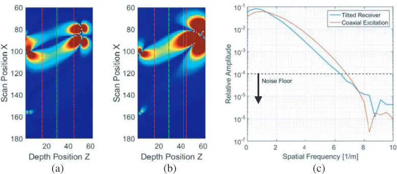
Figure 2. (a) Calculated H·H sensitivity map for two coaxial and opposing coils with a diameter of “12” and an axial distance of “100” (sign suppressed). The excitation coil is centered at z= “0” and the receiver coil atz= “100”. Although the sensitivity field is symmetric, the exciting field intensity is not: strong fields occur toward the left excitation coil. At high power levels, a safety distance toward the left must be considered for biomedical applications, here arbitrarily set to z= “40” (red trace). A second border is generally applied toward the right sensor coil (z = “85”), as even small objects very close to the sensor cause relatively strong signals, thereby masking objects in the less-sensitive middle region. (b) A very similar sensitivity map from the given safety border toward the right receiver can be obtained using a larger excitation coil (diameter “55”) with a less-concentrated field and placing it closer (z= “30”) to the safety border.
up to 60µT for a short period of time [22]. At high power, regions with field intensities that exceed the guidelines must not be used for biomedical applications. In our example, a safety border is arbitrarily set to z= “40”. For a biomedical MIT, the only parts that remain are the diffuse region in the center and the more concentrated area toward the receiver. In such a high-power situation with an additional safety border, the small and very strong excitation coil atz= “0” can be replaced by a larger excitation coil (diameter = “55”) with a less concentrated field (Fig. 2(b), now better approaching the situation in Fig. 1). It can be placed closer (z = “30”) to the safety border: the resulting H ·H sensitivity field toward the sensor (z = “50. . .100”) remains mostly unchanged. The closer, larger, and less field-concentrating excitation coil can be powered more easily toward the permissible flux density at the designated border.
The excitation coil can be equipped with an additional loop with a somewhat larger diameter (Figs. 1(a) and (b)) and driven exactly in the counterphase, resulting in a coaxial gradiometer, as suggested in a previous contribution [23]. As an exciter, a coaxial gradiometer is believed to provide a sensitivity field (preliminary just H·H) toward the receiver with fewer axial gradients and increased radial gradients. Both properties should improve the signal quality (e.g., enhance the higher spatial frequencies) from a scan in the lateral direction. This additional loop also decreases the excitation field in the measurement volume via destructive interference, although the limit of 10µT at the designated safety border can be readily maintained.
(a) (b) (c)
Figure 3. (a) Calculated H ·H sensitivity map (absolute amplitudes, sign suppressed) in the x-z plane with a large and coaxial excitation gradiometer and a smaller and normally oriented receiver coil in a lateral offset position, representing the geometries in Fig. 1. Borders are indicated toward the left and the right (red traces). (b) A nulling of the primary field can also be achieved with merely a single excitation loop and a tilted receiver. However, in the most diffuse middle region with the weakest response the lateral (x-direction) gradients are lower and the axial gradients are higher toward the sensor. (c) FFT analysis of calculated signals from a travelling “dot” in the middle region, at
z = 30 (green trace in (a) and (b)). With the same flux density at the left excitation border, the coaxial gradiometer provides relatively enhanced signal components at higher spatial frequencies. The generally strong low pass behavior remains a challenge. The discrete x-positions in the virtually exact calculation digitally cause noise floor below amplitudes of 104.
and then with a strong primary signal. The resultingH·H map is then similar to Fig. 3(b). This could be calculated, yet an experimental verification is not possible with the herein used receivers.
The formulations for theH·Hmapping, theE·J forward modeling of interconnected objects, and the general field intensities use analytical expressions (obtained from [24]) with the complete elliptic integrals EE and K. Normally, the EE is stated as a single “E” which here would collide with the induced electrical field E. The equations provide the axial (Hz) and the radial (Hr) field intensity as well as the more commonly known vector potential (Aϕ) from a circular current loop with radius R, currentI, and centered at z= 0 for any point in the space (r, z):
Hr(r, z) = Iz 2πr
m
4Rr
2−m
2−2mEE(m)−K(m)
(1a)
Hz(r, z) = I 2πr
m
4Rr
rK(m) +Rm−(2−m)r
2−2m EE(m)
(1b)
Aϕ(r, z) = μπ0I
R rm
1−m
2
K(m)−EE(m)
(1c)
m = 4Rr
z2+ (R+r)2 (1d)
To compute a more rigid E ·J forward description for interconnected and extended bodies, we applied the induced electrical field components E in the space — proportional to the exciting loop’s vector potential Aϕ from Eq. (1) — to a 3D (or 2D) resistor grid similar to [19] with, e.g., 1000 nodes, representing a voluminous and interconnected body (or conducting sheet). The equation system was solved for the individual eddy currentsJ inside this grid in thex,y, andzdirections. As is already well-known for MIT methods, this particular operation imputes a relatively high computational cost. Here it must even be carried out for eachx-position in the scanning process. Then, the inner product (E·J) of the local eddy currents J in the body and a virtually-induced E field of the corresponding receiver coil sum up to the simulated receiver signal [17]. For a body with 1000 nodes, a current standard office PC with MATLAB requires approximately 50 seconds for a virtual scan with 256 x-positions. Because the forward problem must be repeatedly solved in MIT imaging until satisfying convergence (virtual signals approach the real sensor signals), efficient coding and fast computing are required for acceptable image delays; such delays should last no longer than a few seconds with such a quick scanner. Sophisticated computation, however, is not the primary objective of this more hardware- and signal-oriented contribution. As will be shown in our calculations and experiments, the much simpler H·H approach suffices here as a preliminary working base, even for local deviations inside voluminous saline bodies.
When considering a distribution O(x, z) of unconnected and point-like metal or ferrite objects in the x-z plane, the received signal function S(x) from an individual sensor caused by a scanning procedure through theH·H sensitivity fieldC(x, z) in thex-direction is simply the sum of convolutions in the x-direction between the object field O and the sensitivity map C. Inside the computer, the one-dimensional convolution of these two arrays can be replaced by multiplying both discrete Fourier transformed functions, here noted with the prefix “f” and spatial frequency ξ in the x-direction. A signal therefore can be modeled and artificially generated in the computer as follows:
fS(ξ) =
n
z=1
fO(ξ, z)·fC(ξ, z) (2)
The summation in thez-direction must include the used space between the excitation and receivers in the scanner. A later required deconvolution of the sensor signal into an image plane I(x, z) for reconstruction purposes can be obtained by multiplying the Fourier transformed signal S with the reciprocal Fourier components of the sensitivity fieldC, as expressed in Eq. (3). However, the reciprocal Fourier components of the sensitivity field describe a very steep high pass — reciprocal to the distinct low-pass behavior of the sensitivity fields (Fig. 3(c)). To obtain practically useful information from real measurement signals with included noise, the higher spatial frequencies with very high gain must be truncated or dampened to tolerable levels. The better the signal quality in terms of artifacts, SNR, and linearity, the higher the truncation level can be set. Tuned with the parameterskandα, this dampening of higher frequencies relates to the commonly-applied regularization of ill-posed inverse problems.
fI(ξz) = fS(ξ)· 1
fC(ξ, z) · ⎛ ⎜ ⎜
⎝ k
k+ 1
|fC(ξ, z)| ⎞ ⎟ ⎟ ⎠
α
(3)
The back-transformed I(x, z) represents the perspective of an individual sensor regarding the original object distribution O(x, z). A single sensor signal comprises the summed response from all depth levels. A depth resolution can only be obtained with at least a second sensor and with a preferably very different projection. Nonetheless, the intended openness of the presented scanner in the x- and
y-directions and the gradiometric operation restricts the free choice of sensor positions and prevents elevated “viewing” angles with respect to the z-axis. The characteristic“viewing” angle of a sensor can be seen from an individualI(x, z) representation (Fig. 4). The current utilization of merely two sensors with crossing perspectives I1 and I2 permits object depth estimation. The simplest approach for an
image-like 2D presentation was obtained by adding the two crossing perspectivesI1 andI2, reminiscent
(a) (b) (c)
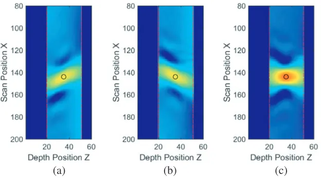
Figure 4. (a) and (b) Calculated projectionsI1 and I2 from Eq. (3) of the two sensors for a single and
point-like object (small circle) in thex-zplane. Considerable dampening for higher spatial frequencies was applied intentionally, and the projections are therefore rather blurred. (c) The addition of the two projections reveals a maximum intensity at the actual location of the object. Due to the “viewing” angles of the sensors, the spatial resolution is better for the scanning direction than the depth.
The resulting patternI1+I2 (Fig. 4(c)) could be introduced into a virtual measurement (Eq. (2)),
and the difference between virtual signals and the actual received original signals, the error, could be processed toward minimization for a subsequently more corrected and iterative reconstruction procedure. This possibility with a relatively low computational cost represents one approach to the inverse problem within the limits of theH·H approach.
Reconstructions for extended and interconnected bodies must implement the forward problem with, for instance, a complete E ·J forward calculation of a computer-estimated body and an inverse and stepwise correction of this body. Interestingly, although Eq. (3) was derived for the H·H approach, it also locates deviations in extended and interconnected bodies.
This effect is calculated initially with a thin and conductive sheet (only 2D figures for a better presentation of eddy currents, Fig. 5), which extends in thex- andy-directions. The general conductivity distribution in the sheet can be inhomogeneous. A small area at the height of the excitation coil and at the outer left x-position of the sheet is modified intentionally. In this example, the local conductivity of the deviation is set to zero. Figs. 5(a) and (b) show the discretized eddy current solutionsJ for the two deviating sheets. The difference between these two eddy current solutions is shown in Fig. 5(c). The deviating eddy currents, as intuitively expected, concentrate around the intended defect. For comparison, the conductivity difference between the two sheets is merely a small and conductive platelet, and the eddy current solution for this small and isolated area and within this discretization is merely a local ring (Fig. 5(d)). Both eddy current fields (Figs. 5(c) and (d)) are obviously deviating. However, when calculating the received signal traces (E·J) over a scan from the then dynamic and multiple eddy current solutions (Figs. 5(c) and 5(d)) in a sensor coil, the obtained signals from scans in the
x-direction are generally quite similar. As a particularly noteworthy difference, both signals occur at deviating x-positions. The signal from the eddy current differences appears somewhat earlier, i.e., at higherx-positions pointing more toward the middle of the sheet. This x-shifting is actually smaller for 3D objects due to the faster decay of the deviating eddy currents toward a 3D volume rather than to a 2D plane.
(a) (b) (c)
(d) (e)
(f) (g)
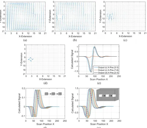
Figure 5. (a) A typical eddy current solution J of a heterogeneously conducting 2D sheet inside the relatively large induction field. (b) The eddy current solution of the locally-modified sheet: the conductivity of a small area near the left edge was set to zero. (c) The difference between the two eddy current fields. (d) The eddy current solution of the conductivity difference is merely a current ring around the small area. (e) Calculated signals (E ·J) in a receiver loop from the dynamically changing eddy current fields (c) and (d), when moving the sheet in the x-direction through the virtual scanner with the inhomogeneous excitation field. Despite the highly deviating results in (c) and (d), the obtained signals are quite similar, albeit displaced in the x-direction. A much smaller response is obtained for a deviation near the middle of the sheet. (f) 3DE·J calculation of the scanner signal and from a small and conducting cube at stepwise changedx-positions. (g) Quite similar differential signals are obtained for a non-conducting void at the same positions inside a generally conducting cuboid, when stepwise positioned from the left inner surface through the middle toward the right inner surface. Even in the middle, the signals are still comparably strong.
and have near-constant amplitudes, albeit the void’s signals are displaced slightly toward the middle of the cuboid. Only negative differential signals would appear for Fig. 5(g) when inserting a better conducting cube instead of a non-conducting void (not shown here). According to Fig. 5(f) and 5(g), similar behaviors were observed for the experiments. For this scanner with moving test objects, the sensitivity for a local deviation inside an extended 3D object apparently does not depend strongly on the deviation’s position. This finding is helpful, as static sensitivity fields for opposing coils tend to show heterogeneous sensitivity and obtain relatively weaker signals from a deviation in the middle of a conducting body (e.g., as shown in [3, 25], and [26] and as seen for the sheet Fig. 5(e)). Thus, as a preliminary working base for this scanner, a differential measurement of a local deviation somewhere in a voluminous and conducting body causes similar signals as the isolated defect alone and without a conducting background. Therefore, a H·H inversion of a differential measurement through Eq. (3) should point to the local deviation or “defect” inside a conducting volume. In addition, the relative gain for higher spatial frequencies with the coaxial gradiometer (Fig. 3(c)) should apply for signals from extended and interconnected bodies.
Therefore, we now continue with the rather simple H ·H approach. Additional attempts with MIT theory are not intended at this stage: this contribution focuses on the technical performance of this scanner. Without sufficient signal integrity — affected by SNR, incident EMI, a capacitive instead of inductive coupling, drift, nonlinearities, and motion/displacement artifact — an intended imaging technique will fail to satisfy the requirements of the delicate MIT methods.
2.2. Practical Techniques
In this section, we describe the techniques for such large, powerful, stable, and gradiometric arrangements with near-complete primary nulling at 1.5 MHz. Therefore, the sensor techniques at the other side of the scanner are less demanding and readily deliver reasonable signals from even low-conductivity and relatively small test bodies. The observed signals from isolated and point-like metal objects or from extended low-conductivity bodies shall then be assessed in terms of signal integrity (SNR, linearity, drift, motion artifacts) and properties or spatial information.
The primary loop consisted of a 15-cm wide, flat, and single-turn copper ring with an outer diameter of 55 cm. With 8 inserted 3.3 nF capacitors (about 26 nF in total), it became a parallel LC-resonator at 1.25 MHz. The LC system was charged continuously with current pulses at 1.25 MHz from a single IRF630 MOSFET (International Rectifier, www.irf.com) and with up to 85 V and 0.1 A. In the designated resonance case, the ring was energized to amplitudes of up to 85 V and then 18 A (I =ωUC). The achieved flux density B somewhere in space was readily measurable as an induced voltage signalUI from a small copper loop with defined cross sectionALand at defined angular frequency (UI =ωBAL). Near the designated safety border and with a somewhat reduced charge voltage, the field can be tuned to 10µT (10% accuracy), and the general SAR safety requirements are fulfilled (even up to 60µT is permitted in Germany for short exposure times [22]). Quite similar flux densities are calculated analytically with the geometrical sizes and current (Eq. (1)).
The current inside the excitation ring was held virtually constant with the relatively weak but continuously recharging pulses from the MOSFET circuitry. The excitation ring was almost completely decoupled from the environment and from any test objects over the safety distance. The excitation was not actively stabilized, which could be improved in the future. Even when perfectly nulling the primary signal in the receivers, a varying or drifting power level could cause varying amplitudes in the received signals. However, this issue could be identified with repeated measurements, and at present, it seems to lack urgency. Importantly, the kW power in the ring could not eventually harm a human being: instead, the maximum available power from the system is smaller than the provided driving power, here in the order of less than 8 W = 85 V∗0.1 A. Since approximately 20 kg of human body mass is exposed to the high field zone with a maximum available power of 8 W, an average SAR can be roughly estimated and is distinctively less than 0.5 W/kg lasting for merely a few seconds. This figure is less than the currently recommended SAR for cell phones (<2 W/kg).
the other side. Fine tuning was done with manual sub-mm shifts of the receivers. The residual phase difference between the two opposing excitation loops cannot be nulled with merely geometrical shifting. Instead, it had to be compensated for with parallel resistors (then phase shifting) at the larger loop. The resistors — loaded with up to 85 V — considerably increased the required driving currents and power toward 20 W and heated up. The resistors must be sufficiently dimensioned for such power dissipation. These measures achieved a virtually complete nulling for the sensors. The balance was stable over hours and not notably affected by changes in the excitation power from the MOSFET driver.
The sensor loops comprised a single and wide winding of approximately 11 cm in diameter and with an integrated transistor amplifier (voltage gain ≈ 50). One side of the sensor ring was defined as the ground potential (= connected to the shield of the signal’s coax cable), and this was used to shield the other side of the ring until half circumference. The single and wide winding resulted in a low impedance behavior for the ring. Together with the shielding, this behavior effectively suppressed the highly undesirable influence of capacitive coupling [27]. A parallel capacitor was inserted to tune the ring resonance distinctively below the operation frequency of the excitation side. With this low-pass behavior, the sensors attenuated overtones from the excitation side generated by the recharging current pulses from the driving MOSFET.
The complete system, and particularly the receiver site, was not shielded against electromagnetic interference (EMI) from the environment (Fig. 1(b)). An essential requisite, the excitation system and the sensor system were mechanically decoupled from the trolley’s rail system. Small vibrations in the excitation or sensing structures would cause relatively large artifacts.
The pre-amplified signals from the receivers were connected to the popular RF mixer/demodulator SA602 (identical to NE612 or NE602). With the reference frequency, the signals were demodulated directly down to DC. The reference signal was obtained through an optical fiber from the excitation side because copper cabling was undesired between powerful excitation and sensitive detectors. The reference phase was tuned to match the phase characteristics of test objects (resistive saline bodies vs. mostly inductive metal objects). The balanced output of the mixer was amplified up to +/−2.5 V and shifted to an offset level of 2.5 V. It then fit well to a common 0–5 V ADC with 12-bit resolution and was recorded in the computer. The scanning trolley’sx-coordinate for the signals included 256 discrete positions and a 0.8-cm distance between the two subsequent positions, resulting in a total travel path of almost 205 cm. The position was sensed optically and transmitted via a dielectric optical fiber.
Extended test bodies with a generally conductive background were made from a 12-liter saline bath in an oval bucket, with a cross-section fairly similar to the human thorax. The water level was covered with a Styrofoam plate to suppress swashing or surface waves (relatively strong and undesired motion artifacts) during a scan. For differential measurements, a better-conducting saline-agar body or a non-conducting void with a relative small volume of approximately 0.23 liters was fixated and fully immersed at various positions inside the volume of the bath. Although the conductivity of the saline bath was considerably higher than the characteristic conductivity of biological tissue [28], the signal level from merely 12 liters is comparable to the levels from a person composed of more volume.
3. EXPERIMENTAL RESULT
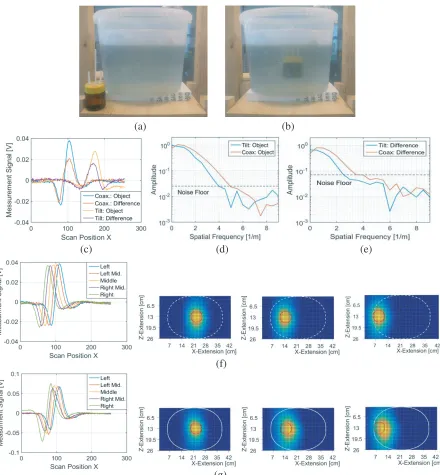
The experimental H·H map or the point spread function (PSF) in the x-z plane was obtained by scanning a “point-like” aluminum tube. The tube was 1 cm in diameter and 10 cm in length (orientated in the y-direction and centered at y = 0) in different z-positions or depths (Fig. 6). A subsequent photograph illustrates the actual appearance of the aluminum test body. The two gradiometric modalities — tilted sensor vs. coaxial excitation — were found to be closely related to the theoretical
(a) (b) (c)
(d) (e)
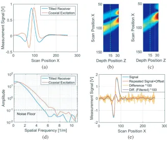
Figure 6. (a) Experimental signals (only from one sensor for clarity) from a single and small aluminum object in the most diffuse and weak-responding middle (here: z = 15) of the MIT zone for the two different gradiometric modalities and at same flux density at the safety border. The experimental sensitivity maps or PSF for the two cases (b) and (c) are closely related to the theoretical H ·H predictions in Fig. 3. The spectrum (d) of the two experimental signals (a) for the coaxial gradiometer shows that relatively higher spatial frequencies can be used for reconstruction (Eq. (3)). Here, a truncation or dampening of the spectral components somewhere below an amplitude of 10−1 is required (i.e., the noise floor). (e) A characteristic repeatability of signals from the metal object closer to the sensor (then exploiting the full linear range of the receivers) points to relatively low artifacts. A numerical offset was added to one measurement for better representation. The unfiltered and filtered signal differences between repeated scans were amplified by 100 times.
should cause fewer artifacts because there are fewer gradients in this direction. This aspect, however, is not further analyzed here.
For the experimental signals, the spectral analysis (spatial frequencies in thex-direction) generally shows a very strong low-pass behavior. As predicted (Fig. 3(c)), a relative advantage emerges at higher spatial frequencies for the coaxial gradiometer. This relative gain is obtained with the same level of flux density at the safety border toward the excitation. From the powerful excitation field, there is a stable and virtually noise-free “pre-differentiation” in that the coaxial signal is similar to the negative first derivative of the tilted receiver signal. This aspect is of interest: a separate measurement with two different and conventional excitation coils followed by taking the numerical difference between the signals could not be performed in this manner. Aside from the lower signal energy (limited excitation due to SAR restrictions), the drift and the noise in the delicate raw signals would fully impinge on a subsequent difference. For an inversion with the reciprocal of these maps (Eq. (3)), it is only possible to utilize those components significantly above the noise floor. The coaxial gradiometer offers higher spatial frequencies above the noise floor, directly effective for localization or resolution. It remains unknown whether such gains are actually conserved for extended saline objects.
repeated-measurements procedure. The difference between the two repeated measurements (measured within about 50 seconds) was 49 dB below a single measurement at full bandwidth (= for the unfiltered raw signals) and 55 dB with a removal of the higher and practically useless spatial frequencies. Therefore, within a single scan of slightly over 5 seconds instead of a repeated scan within 50 seconds, the figure of merit for artifacts is at least 3 dB higher than 55 dB. This could likely be further increased in the future with, for instance, shielding measures against EMI and more matured and better stabilized electronics/mechanics. As a preliminary conclusion, artifacts from mechanical or electronic noise seem to be an insignificant issue for inanimate test objects in this scanner.
Using Eq. (3a), difference measurement between intentionally modified and discrete metal arrangements can be used to localize the modification itself (Fig. 7). At the same time, the difference between the two measurements is generally very similar to merely a single object at the position of difference. Therefore, a weak coupling approach can be stated here: the ubiquitously present primary field is obviously much stronger than the effected field perturbation from the individual and relatively small metal objects. Otherwise, such linearity could not work.
(a) (b)
(c) (d) (e)
7 14 21 28 35 42 0
Figure 7. Coaxial gradiometer. (a)–(c) The difference between the measurements of two distinctively different metal patterns (the deviation: a missing object at position #3) is closely related to a measurement of (d) a single object at the difference position (only one sensor signal is shown for clarity). (e) Therefore, a localization in thex-z-plane with the two crossing projections (related to Fig. 4(c)) of the difference signals between the two settings (a) and (b) obtains a maximum near the position of the difference.
The response from an extended object was tested with the two different gradiometric setups. A bucket with 12 liters of 1.5% saline was repeatedly scanned. The bucket provides a roughly similar cross-section as a human thorax. Although the bucket’s general conductivity is much lower than the above-used aluminum samples, the much larger volume results in comparably strong signals.
(a) (b)
(c) (d) (e)
(f)
(g)
with deionized water, Fig. 8(a)) can be tested. For proper signals, the same volume of saline has to be removed when inserting the local inhomogeneity in the bath; in essence, the general volume or filling height of the test body should remain unchanged. The differential detection of the inhomogeneity’s signature inside the saline was readily possible. Thereby, an inductive sensing through the saline’s volume can be stated, rather than just a capacitive coupling to surfaces. A capacitive effect would interact primarily with the surface of the conducting and high-permittivity saline bat; it would hardly extend into the depth. It is also possible to conclude the reasonable reproducibility of subsequent mechanical scans, similar to the metal objects above (Fig. 6(e)), but not repeatedly shown here. As can be expected with equal geometries, a relatively better-conducting agar object inside the saline bath produces the negative differential response of a non-conducting void (not shown here).
More interesting and according to the E ·J calculations of Figs. 5(f) and 5(g), the differential signature of the 0.23-liter void inside the saline is related to the negative response of the same glass alone. This behavior occurs without any conducting background, and at the same position, when filled with conducting saline. This behavior is fairly true for various positions inside the saline bath, and the signal amplitudes do not significantly depend on the position of the deviation (middle vs. near wall), similar to the calculated Fig. 5(g). As already seen with Fig. 5, the difference signals appear somewhat and systematically shifted toward the center of the bucket. Thereby, a geometrical mismatch is obtained for a “back projection” via Eq. (3). The spatial spectra of the small signals generally show lower useful frequencies with respect to Fig. 6(d), as the glass with a diameter of 6.5 cm already provides a lateral extension (it is not a “point” anymore). Meanwhile, the (differential) signals from the 0.23-liter saline volume are much smaller than those of the aforementioned aluminum objects, thereby closer to the scanner’s limiting noise floor. As an experimental result from Fig. 6(d), the gain for higher spatial frequencies for extended bodies is still present with the coaxial excitation gradiometer.
The differential signals from the saline bucket were introduced into the H·H inversion, and the obtained projections point to the approximate position of the deviation (Fig. 8(g)), although they are somewhat displaced toward the center of the bucket. No significant displacement is obtained for the saline filled glass alone (Fig. 8(f)).
Relevant for MIT applications with living beings, difference measurements were performed with the authors as test subjects. The flux density at the safety border toward the excitation side was set to the permissible SAR level of 10µT at 1.5 MHz. Although a generally lower conductivity than 1% saline is known for human tissue [25], an upright standing human provides much more conducting volume to the measurement zone due to a more widely-extending y-direction. The obtained signal level from a person therefore was relatively strong and exploited the full linear scale of the receivers (Fig. 9). During a scan, any unintended motions or changes in the respiratory condition (breathing) of the test person are relevant. The difference between two subsequent scans without intentional changes made by the test person provides a worst-case level for artifacts. The figure of merit was found to be in the order of 44 dB. A better signal integrity can be expected — although without explicit proof here — within a single scan. This expectation results from the fact that a person’s displacement and deviating respiratory condition between two subsequent measurements occurring over a longer period of time of about 50 seconds and with breathing between scans will typically be stronger than within a shorter time frame, traveling through the MIT zone (5 seconds and with respiratory arrest). Furthermore, it should be noted that the person in the experiment was standing in an upright and self-stabilizing posture and was not deliberately immobilized in the trolley (Fig. 1).
(a) (b)
Figure 9. (a) A sequence of four subsequent measurements from a test person (Fig. 1(b)) and with alternating respiratory states. The signals are relatively strong and well exploit the linear range of the receivers. In the first and third measurements, the person was in a distinct inspiration state; in the other two measurements, the person was in an expiration state. (b) Over the measurement sequence, the intended difference between expiration and inspiration states is significantly higher than the unintended difference (= artifacts) between two expiration states.
(a) (b)
Figure 10. (a) Differential measurement of an intentional change, photographed with deactivated excitation and a removed security spacer. An additional and relatively small agar object is attached to the left outside of the upper thorax, at the height of the excitation and sensor axis. (b) TheH·H inversion of the difference signals (with and without agar) points to the virtually correct x-position of the agar.
the scanner. Due to the complex 3D features and displacements inside the thorax, a simple differential reconstruction similar to Fig. 8(f) (only a simple 2D “back projection”) does not obtain meaningful representations here.
4. DISCUSSION
This mechanical scanner with high excitation power allows — currently only via difference measurements — the quick detection and localization of perturbations inside a generally conducting background of larger objects. The exclusively gradiometric operation was achieved with two different methods, via a coaxial excitation system and with tilted sensor loops. The received signals directly exhibited the signatures of either inductive (metals) or resistive (saline) perturbations. Both the excitation and the sensor loops were made from a single and wide winding, thereby obtaining low-impedance behavior for both sides. Low impedance levels, i.e., high currents at relatively low voltages, help to improve the magnetic or inductive coupling (currents) in relation to the highly undesirable coupling via electric fields (voltages).
The coaxial gradiometer provides somewhat better localization and higher spatial frequencies in the scan direction, as calculated and practically obtained for the particularly interesting and critical center zone: the middle represents difficult-to-access areas deep inside the body and at the same time the signal response from this zone is relatively weak and most diffuse (Figs. 6(b) and (c), green trace). In addition, the correspondingH·Hsensitivity shows a lower gradient in the axial “viewing” direction, making signals from the near sub-surfaces lightly stronger than signals from the deeper regions. Based on the calculations and experiments, these improvements from the coaxial excitation gradiometer also apply to extended and generally conducting bodies.
TheH·H inversion through Eq. (3) points to isolated and point-like objects, and it fairly localizes and indicates deviations inside a generally conducting background, here almost irrespective of the position. It remains unclear whether such H·H inversion — which are computer-efficient and thus far useful for this scanner — could be further exploited in the future.
The scanner’s overall reproducibility is already promising: displacement or motion artifacts even over subsequent scans seem to be insignificant for inanimate test objects (58 dB). The scanning of a living being, here an upright standing and not distinctively fixated human being, point to more pronounced artifacts over two subsequent scans (44 dB). These artifacts, however, are much weaker (27 dB) than the signal deviations from intended and distinct breathing activity, i.e., an imprint of features mainly from inside the thorax. We expect that a characteristic displacement error from a human within the 5 relevant seconds in a single scan would be lower.
In potential future systems and with a generally vertical arrangement of the measurement technique, a patient could lie in a stabilizing recess, and the signal integrity should be even better. Non-metallic motion sensors (e.g., based on a pneumatic principle) could ensure the motionlessness of the body during the short measurement. More advantageous, a lying person tends to flatten somewhat and, therefore, would allow a smaller gap between excitation (or safety border) and sensing, leading to better resolution. For reconstruction purposes, it would be helpful to know the surface contour of the body, since then — as a priori knowledge — no conducting material and no eddy currents would be present at locations outside the body. A surface contour could be registered with relatively simple optical methods during the scan.
The current system does not explicitly optimize geometries for the exciting and receiving. It is unlikely that the current geometries already present an optimum. With the given SAR limit for humans and a computer modeling of the MIT effects, the sizes and the positions of the loops should be further refined to ensure the best possible detection and resolution in the MIT zone.
Because the currently-used coaxial gradiometer with two well-balanced current loops performs a noise-free and apparently helpful “pre-differentiation” of the signals (i.e., the coaxial signal is similar to the first derivative of the signal with the tilted receiver), a more general question arises: Would more coaxial excitation loops (and/or loops with other geometries) with opposite phase relations a) perform even better for the MIT volume and b) be practically realizable?
This contribution used only two sensors in the x-z plane. However, the number of applicable sensor loops with other projections and with y-information for 3D can be much higher. In the coaxial excitation gradiometer, normally-orientated sensors can only be placed in a distinct radius around thez -axis for primary field cancellation. Even more and then tilted sensors at other positions could be added. Additional sensors could even be placed at the excitation site, which would then better approach the object of interest from the other side, thereby offering more resolution in thez-direction.
forward model and real bodies, which is a precondition [30] for image reconstructions from voluminous bodies. Aside from additional and improved (balanced and symmetrical and fully shielded) sensor loops, a real medical question could be addressed. At the moment, the scanner seems to hold promise in evaluating certain lung diseases [29] because the lungs are relatively voluminous organs and therefore more suitable for the generally low-resolving MIT methods. In addition, the lungs allow intentional changes via respiration.
In its current state, the scanner deviates in many aspects from currently-described MIT systems, and it might offer a practical chance for a 3D assessment of extended objects or even human beings.
ACKNOWLEDGMENT
The corresponding ethics committee in Duesseldorf (Germany) stated (May 22th, 2017, Ref. 118-2017) that a formal approval currently is not required, because a) no specific physiological feature or medical study is assessed, and b) no physician is involved in this study
The SAR limit for non-ionizing energy was not reached [22] and was also inspected by the local safety officer. No other and extraordinary risk potential for humans was apparent.
This work was supported by internal funding from the authors’ institution and by the Deutsche Forschungsgemeinschaft contract RU 2120/1-1 “INDIGO”.
REFERENCES
1. Wei, H. and M. Soleimani, “Electromagnetic tomography for medical and industrial applications: Challenges and opportunities [Point of view],” Proceedings of the IEEE, Vol. 101, No. 3, 559–565, 2013.
2. Dekdouk, B., C. Ktistis, D. Armitage, and A. Peyton, “Absolute imaging of low conductivity material distributions using nonlinear reconstruction methods in magnetic induction tomography,” Progress In Electromagnetics Research, Vol. 155, 1–18, 2016.
3. Wei, H. and M. Soleimani, “Hardware and software design for a national instrument-based magnetic induction tomography system for prospective biomedical applications,”Physiological Measurement, Vol. 33, No. 5, 863–879, 2012.
4. Scharfetter, H., S. Issa, and D. G¨ursoy, “Tracking of object movements for artefact suppression in Magnetic Induction Tomography (MIT),”Journal of Physics: Conference Series, Vol. 224, 012040, 2010.
5. Zolgharni, M., H. Griffiths, and P. Ledger, “Frequency-difference MIT imaging of cerebral haemorrhage with a hemispherical coil array: Numerical modelling,” Physiological Measurement, Vol. 31, No. 8, S111–S125, 2010.
6. G¨ursoy, D. and H. Scharfetter, “Reconstruction artefacts in magnetic induction tomography due to patient’s movement during data acquisition,” Physiological Measurement, Vol. 30, No. 6, S165– S174, 2009.
7. Watson, S., R. Williams, W. Gough, and H. Griffiths, “A magnetic induction tomography system for samples with conductivities below 10 S m−1, Measurement Science and Technology, Vol. 19, No. 4, 045501, 2008.
8. Rosell-Ferrer, J., R. Merwa, P. Brunner, and H. Scharfetter, “A multifrequency magnetic induction tomography system using planar gradiometers: Data collection and calibration,” Physiological Measurement, Vol. 27, No. 5, S271–S280, 2006.
9. Vauhkonen, M., M. Hamsch, and C. Igney, “A measurement system and image reconstruction in magnetic induction tomography,” Physiological Measurement, Vol. 29, No. 6, S445–S454, 2008. 10. Wei, H. and M. Soleimani, “Three-dimensional magnetic induction tomography imaging using a
matrix free krylov subspace inversion algorithm,”Progress In Electromagnetics Research, Vol. 122, 29–45, 2012.
12. Wei, H., L. Ma, and M. Soleimani, “Volumetric magnetic induction tomography,” Measurement Science and Technology, Vol. 23, No. 5, 055401, 2012.
13. Wei, H. and M. Soleimani, “Two-phase low conductivity flow imaging using magnetic induction tomography,”Progress In Electromagnetics Research, Vol. 131, 99–115, 2012.
14. Ma, L., H. Wei, and M. Soleimani, “Planar magnetic induction tomography for 3D near subsurface imaging,”Progress In Electromagnetics Research, Vol. 138, 65–82, 2013.
15. Wei, H. and M. Soleimani, “Theoretical and experimental evaluation of rotational magnetic induction tomography,”IEEE Transactions on Instrumentation and Measurement, Vol. 61, No. 12, 3324–3331, 2012.
16. Dekdouk, B., C. Ktistis, W. Yin, D. Armitage, and A. Peyton, “The application of a priori structural information based regularization in image reconstruction in magnetic induction tomography,”Journal of Physics: Conference Series, Vol. 224, 012048, 2010.
17. Ktistis, C., D. Armitage, and A. Peyton, “Calculation of the forward problem for absolute image reconstruction in MIT,”Physiological Measurement, Vol. 29, No. 6, S455–S464, 2008.
18. Rosell, J., R. Casanas, and H. Scharfetter, “Sensitivity maps and system requirements for magnetic induction tomography using a planar gradiometer,”Physiological Measurement, Vol. 22, No. 1, 121– 130, 2001.
19. Morris, A., H. Griffiths, and W. Gough, “A numerical model for magnetic induction tomographic measurements in biological tissues,” Physiological Measurement, Vol. 22, No. 1, 113–119, 2001. 20. Scharfetter, H., P. Riu, M. Populo, and J. Rosell, “Sensitivity maps for low-contrast perturbations
within conducting background in magnetic induction tomography,” Physiological Measurement, Vol. 23, No. 1, 195–201, 2002.
21. International commission on non-ionizing radiation protection (ICNIRP): Guidelines for limiting exposure to time-varying electric, magnetic and electromagnetic fields (up to 300 GHz), published at www.icnirp.org.
22. IFA Report 3/2017, Grenzwerteliste 2017, Sicherheit und Gesundheitsschutz am Arbeitsplatz, published at www.dguv.de.
23. HeidaryDastjerdi, M., D. R¨uter, O. Kanoun, and J. Himmel, “Induktionsfelder mit vorteilhaften Topologien in der Magnetischen-Induktions-Tomografie,” TM — Technisches Messen, Vol. 80, No. 11, 2013.
24. Good, R., “Elliptic integrals, the forgotten functions,”European Journal of Physics, Vol. 22, No. 2, 119–126, 2001.
25. Scharfetter, H., R. Merwa, and K. Pilz, “A new type of gradiometer for the receiving circuit of Magnetic Induction Tomography (MIT),” Physiological Measurement, Vol. 26, No. 2, S307–S318, 2005.
26. Hollaus, K. J., C. Magele, R. Merwa, and H. Scharfetter, “Fast calculation of the sensitivity matrix in magnetic induction tomography by tetrahedral edge finite elements and the reciprocity theorem,” Physiological Measurement, Vol. 25, No. 1, 159–168, 2004.
27. Griffith, H., W. Gough, S. Watson, and R. J. Williams, “Residual capacitive coupling and the measurement of permittivity in magnetic induction tomography,” Physiological Measurement, Vol. 28, No. 7, S301–311, 2007.
28. Faes, T. J. C., H. A. van der Meij, J. C. de Munck, and R. M. Heethaar, “The electric resistivity of human tissues (100 Hz–10 MHz): A meta-analysis of review studies,” Physiological Measurement, Vol. 20, No. 4, R1–10, 1999.
29. Rueter, D., H. P. Hauber, D. Droemann, P. Zabel, and S. Uhlig, “Low frequency ultrasound permeates the human lung in situ: A novel method for lung testing,”Ultraschall in Med., Vol. 31, No. 1, 53–62, 2010.