e-Publications@Marquette
Electrical and Computer Engineering Faculty
Research and Publications
Electrical and Computer Engineering, Department
of
10-1-2010
Cluster-Based Distributed Face Tracking in Camera
Networks
Josiah Yoder
Purdue University
Henry Medeiros
Marquette University, [email protected]
Johnny Park
Purdue University
Avinash Kak
Purdue University
Accepted version. Reprinted, with permission, from
IEEE Transactions on Image Processing, Vol. 19,
No. 10 (October 2010): 2551-2563.
DOI
. © 2010 Institute of Electrical and Electronics Engineers
(IEEE).
This material is posted here with permission of the IEEE. Such permission of the IEEE does not in
any way imply IEEE endorsement of any of Marquette University’s products or services. Internal or
personal use of this material is permitted. However, permission to reprint/republish this material for
advertising or promotional purposes or for creating new collective works for resale or redistribution
must be obtained from the IEEE by writing to [email protected]. By choosing to view this
document, you agree to all provisions of the copyright laws protecting it.
Cluster-Based Distributed Face Tracking in Camera
Networks
Josiah Yoder, Henry Medeiros, Johnny Park, and Avinash C. Kak
Abstract—In this paper, we present a distributed multi-camera face tracking system suitable for large wired camera networks. Unlike previous multi-camera face tracking systems, our system does not require a central server to coordinate the entire tracking effort. Instead, an efficient camera clustering protocol is used to dynamically form groups of cameras for in-network tracking of individual faces. The clustering protocol includes cluster propagation mechanisms that allow the computational load of face tracking to be transferred to different cameras as the target objects move. Furthermore, the dynamic election of cluster leaders provides robustness against system failures. Our experimental results show that our cluster-based distributed face tracker is capable of accurately tracking multiple faces in real-time. The overall performance of the distributed system is comparable to that of a centralized face tracker, while presenting the advantages of scalability and robustness.
Index Terms—Distributed Tracking, Object Detection, Face Tracking, Camera Networks.
I. INTRODUCTION
As humans, our faces play a central role in how we com-municate with one another in face-to-face encounters. While the importance of face recognition in such communications is universally known, less widely acknowledged are the roles played by the orientation of a face and the movement of the head that help us understand many aspects of nonverbal communications. The orientation of a face typically indicates the visual focus of attention [1], [2] and can be an important source of information in ascertaining how a person is interact-ing with his/her environment. For example, in an application scenario involving a supermarket, if a computer vision system needed to figure out as to what object a customer was currently looking, the orientation of the face would be a strong indicator of that. Face/head orientation is also used in several important forms of non-verbal communications, such as when a person is nodding his/her head to express agreement, or when a person is shaking his/her head sideways to express the opposite.
The fact that the pose of a person’s face holds important clues as to how he/she is interacting with the environment has motivated several researchers to work on face detection [3], [4], [5], [6], pose estimation [7], [8], [5], [9], [10], [11], [12], and on face tracking [13], [14], [15], [16], [17], [18], [19]. It goes without saying that the ability of a computer system to detect and track people’s faces in real time will open doors to a host of new applications ranging from human-computer interaction to surveillance. The contributions we have cited
Authors are with the School of Electrical and Computer Engineer-ing, Purdue University, West Lafayette, Indiana, 47907, USA. email: {yo-der2,hmedeiro,jpark}@purdue.edu.
above have focused on extracting the needed information from single camera images. However, it stands to reason that simultaneously using multiple images taken from different viewpoints can only lead to more robust estimation of the pose of a face, not to speak of the enhanced ability to track the face/head of a person in motion. Indeed, in the generic context of object tracking, there has been much interest in combining information from multiple cameras [20], [21], [22].
In the existing work on the use of several cameras si-multaneously for estimating the pose of a face, a single computer pulls together either all of the images captured by the cameras or the features extracted from all the images. These centralized approaches to pose estimation and tracking may involve extensive comparisons of the images, as in dense-stereo reconstruction [23] or as in the construction of active appearance models [12], [24]. Such approaches are not easy to implement in a distributed computing environment composed of smart cameras — a theme central to the work reported here. More appropriate for distributed implementations are those prior contributions that use lightweight object features extracted from the individual camera images [25], [26], [27], [28]. Note that these contributions still require a central server to process either all the images or the features extracted from all the images. There are two major shortcomings to all methods that use a single processor for the computation of the face pose: (1) The processor creates a single point of failure and a prominent point of vulnerability in the system; and, perhaps even more importantly, (2) the number of cameras that can be connected to the processor is determined by the capabilities of the processor. For those reasons, our focus here is on face pose estimation and tracking algorithms that, from the ground up, are designed specifically for a distributed implementation.
A distributed approach to the estimation of face pose and to its tracking evidently requires coordination among the camera nodes that are focusing on solving a particular instance of the problem. As is now a common practice in wireless sensor networks, such coordination is best achieved if one of the nodes is chosen to serve as a leader. In wireless sensor networks, a collaborating set of nodes is usually referred to as a cluster and the leader as a cluster head [29], [30], [31], [32], [33]. In this paper, we will use cluster leader or simply
leader to refer to the camera node that is coordinating the
computations being carried out by a collection of camera nodes. This is to avoid confusion with head that, in the present context, is used more appropriately to refer to the anatomical part of the human whose face is the focus of pose estimation and tracking.
In addition to the need for a cluster leader, a distributed approach would also require only those camera nodes that are relevant to the task at hand to participate in pose and tracking computation. That is, assuming a moderate to large network of cameras, we would want only those camera nodes that can actually see a face to try to compute the pose of the face and to contribute to its tracking. As the bearer of the face moves, this collection of the camera nodes must also “move” accordingly. This dynamic formation of a camera node cluster and the subsequent propagation of the cluster requires what is known as a clustering protocol in the jargon of wireless sensor networks [34], [35], [36], [37], [38], [39], [40]. However, these mainstream clustering protocols are only appropriate for non-directional sensor nodes. On account of the non-directional and other unique properties of wireless camera sensors [41], [42], a clustering protocol that is more suited for wireless camera networks is the one we presented in [43]. Our goal in this paper is to show how our clustering protocol can be modified so that it can be used in a network of wired cameras and serve as the underlying framework for the design of a distributed face tracking algorithm.
II. A MULTI-CAMERAFACETRACKINGALGORITHM
We start by presenting in this section a multi-camera al-gorithm for face tracking. Our approach is based on the fact that one can carry out a rough localization of a face, with respect to all its six degrees of freedom (6-DOF), in a single camera image. Estimates of the position and the orientation of a face in the world coordinates, as gleaned from the individual images in a camera network, constitute a set of world-based 6-DOF pose observations for the face. These observations from the individual cameras, along with the uncertainties associated with them, are then integrated in the world coordinates using a minimum variance estimator. A face is tracked in the world coordinates using this integrated estimate.
A. 6-DOF Face Pose Representations
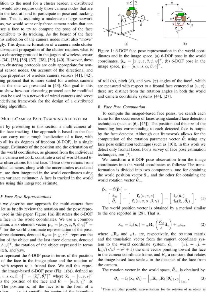
Before we describe our approach for multi-camera face tracking, let us briefly review the notation and the pose repre-sentation used in this paper. Figure 1(a) illustrates the 6-DOF pose of a face in the world coordinates. We use a common representation, a six-element vector˜pw= [x, y, z, θ, φ, ψ]T = [˜xTw,θ˜wT]T for the world-coordinate representation of the pose.
The first three elements, denotedx˜w= [x, y, z]T, represent the
3D position of the object and the last three elements, denoted ˜
θw= [θ, φ, ψ]T, the rotation of the object expressed in terms
of roll, pitch, and yaw.
We also represent the 6-DOF pose in terms of the position and size of the face in the image plane and the rotation of the face with respect to a frontal face. We call this repre-sentation the image-based 6-DOF pose (Fig. 1(b)), defined as
˜ pi = [u, v, s, α, β, γ]T = [˜xTi ,θ˜ T i ] T where x˜ i = [u, v, s]T
represents the position of the face and θ˜i = [α, β, γ]T its
rotation. The position x˜i of the face is in the form of a
bounding-box — (u, v) specify the center of the bounding box andsthe scale. The rotation parameter vectorθ˜i consists
(a) (b)
Figure 1: 6-DOF face pose representation in the world coor-dinates and in the image space. (a) 6-DOF pose in the world coordinates, p˜w = [x, y, z, θ, φ, ψ]T. (b) 6-DOF pose in the
image space,p˜i = [u, v, s, α, β, γ]T.
of roll (α), pitch (β), and yaw (γ) angles of the face1, which are measured with respect to a frontal face centered at(u, v); these are distinct from the rotation angles in both the world and camera coordinate systems [44], [27].
B. Face Pose Computation
To compute the imaged-based face poses, we search each frame for the occurrence of faces using standard face detection techniques (such as [6], [45]). The position and the size of the bounding box corresponding to each detected face is output by the face detector. Although our framework allows for the computation of the rotation parameter vector θ˜i using any face pose estimation technique (such as [10]), in this work we detect only frontal faces. For a survey of face pose estimation techniques, see [7].
We transform a 6-DOF pose observation from the image coordinates into the world coordinates as follows: The trans-formation is divided into two components, one for obtaining the world position vector x˜w and the other for obtaining the
world rotation vectorθ˜w,
˜ pw=f(˜pi) = ˜ xw ˜ θw = fx(u, v, s) fθ(u, v, α, β, γ) = fx(˜xi) fθ(˜xi,θ˜i) . (1) The world position vector is obtained by a method similar to the one reported in [28]. That is,
˜ xw=fx(˜xi) =wRc Ks s dˆc +wtc, (2)
where wRc and wtc are, respectively, the rotation matrix
and the translation vector from the camera coordinate sys-tem to the world coordinate syssys-tem, dˆc = (uˆic +vˆjc + ˆ
kc)/(
√
u2+v2+ 1) the unit vector pointing toward the face
in the camera coordinate frame, andKsa constant that relates
the image-based face scales to the distance of the face from the camera.
The rotation vector in the world space,θ˜w, is obtained by ˜ θw=fθ(˜xi,θ˜i) = h wRc cRl[θ˜i]3×3 i 3×1, (3)
1There are other possible representations for the rotation of an object in world or image-based coordinates. We discuss these in more detail in the conclusions (Sec. VI).
Camera center
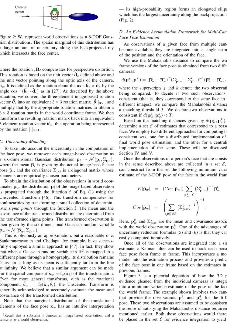
Figure 2: We represent world observations as a 6-DOF Gaus-sian distributions. The spatial marginal of this distribution has a large amount of uncertainty along the backprojected ray which intersects the face center.
where the rotationcRlcompensates for perspective distortion.
This rotation is based on the unit vectordˆcdefined above and
the unit vector pointing along the optic axis of the camera, ˆ
kc. It is defined as the rotation about the axiskˆc×dˆc by the
angle cos−1
(ˆkc ·ˆdc) as in [27]. As described by the above
equation, we convert the three-element image-based rotation vector θ˜i into an equivalent3×3rotation matrix[θ˜i]3×3and
multiply that by the appropriate rotation matrices to obtain a 3×3 rotation matrix in the world coordinate frame. We then transform the resulting rotation matrix back into an equivalent 3-element rotation vectorθ˜w, this operation being represented by the notation[·]3×1.
C. Uncertainty Modeling
To take into account the uncertainty in the computation of the face pose, we represent each image-based observation as a six-dimensional Gaussian distribution pi ∼ N(pi,Σp,i),
where the mean pi is given by the actual image-based2 face
posep˜i, and the covarianceΣp,i is a diagonal matrix whose
elements are empirically chosen parameters.
To obtain the distribution of the observations in world coor-dinatespw, the distributionpi of the image-based observation
is propagated through the function f of Eq. (1) using the Unscented Transform [46]. This transform compensates for nonlinearities by transforming a small collection of determin-istic sigma points through the function f. The mean and the covariance of the transformed distribution are determined from the transformed sigma points. The transformed observation is then given by the six-dimensional Gaussian random variable
pw∼ N(pw,Σp,w).
This is obviously an approximation, but a reasonable one. Sankaranarayanan and Chellapa, for example, have success-fully employed a similar approach in [47]. In fact, they show that when a Gaussian random variable in R2
is mapped to a different plane through a homography, its distribution remains Gaussian as long as its mean is sufficiently far from the line at infinity. We believe that a similar argument can be made for the spatial componentx˜w=fx(˜xi)of the transformation.
Even for more general transforms, such as the rotational component, θ˜w = fθ(˜xi,θ˜i), the Unscented Transform is
generally acknowledged to accurately estimate the mean and covariance of the transformed distribution.
Note that the marginal distribution of the translational elements of the face pose xw has an intuitive interpretation
2Recall that a subscript i denotes an image-based observation, and a
subscriptwa world observation.
— its high-probability region forms an elongated ellipsoid which has the largest uncertainty along the backprojection ray (Fig. 2).
D. An Evidence Accumulation Framework for Multi-Camera Face Pose Estimation
As observations of a given face from multiple cameras become available, they are integrated into a single estimate of the position and the orientation of the face.
We use the Mahalanobis distance to compare the world-frame versions of the face pose as obtained from two different cameras: d(pjw,p k w) = (p j w−p k w) T (Σjp,w+ Σ k p,w) −1 (pjw−p k w), (4)
where the superscripts j and k denote the two observations being compared. To decide if two such observations are consistent (that is, they correspond to the same face in two different images), we compare the Mahalanobis distance to a matching threshold T. We declare two observations to be consistent ifd(pjw,pkw)< T.
Based on the matching distances given by d(pj
w,pkw), we
determine a set E of estimates that correspond to a person’s face. We employ two different approaches for computing these consistent sets, one for a distributed implementation of the final world pose estimation, and the other for a centralized implementation of the same. These will be discussed in Section IV and V.
Once the observations of a person’s face that are consistent in the sense described above are collected in a set E, we can construct from the set the following minimum variance estimate of the 6-DOF pose of the face in the world frame:
E[ˆpw] = (Cov[ˆpw]) X pkw∈E Σk p,w −1 pkw (5) Cov[ˆpw] = X pkw∈E Σkp,w −1 −1 . (6) Here, pk
w and Σkp,w are the mean and covariance associated
with the world observationpkw. One of the advantages of the uncertainty reduction formulas (5) and (6) is that they can be easily computed iteratively.
Once all of the observations are integrated into a single estimate, a Kalman filter can be used to track each person’s face pose from frame to frame. This incorporates a motion model into the estimation process and provides a prediction of the face pose in one frame based on the estimates in the previous frames.
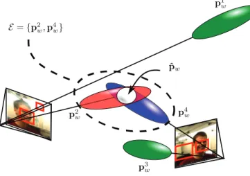
Figure 3 is a pictorial depiction of how the 3D pose evidence gleaned from the individual cameras is integrated into a minimum variance estimate of the pose of the face in the world frame. The example shown involves two cameras that provide the observations p2
w and p
4
w for the 6-DOF
pose. These two observations are assumed to be consistent in the sense of satisfying the Mahalanobis distance requirement mentioned earlier. Both these observations would therefore be placed in the set E for evidence integration to yield the
Figure 3: Evidence accumulation framework. Consistent world observations are found using the Mahalanobis distance. Cor-responding observations are integrated using a minimum vari-ance estimator. The framework is naturally robust to incorrect detections.
minimum variance estimate pˆw. It is important to mention
that this approach is naturally robust to false face detections, as illustrated by the observations p1
w and p
3
w depicted in
the figure. For each such presumably anomalous observation in one camera, the likelihood of there existing consistent observations in the other cameras would be low (except, perhaps, for accidental matchings for the case of images of crowded scenes when each image could include several faces).
III. EVENT-DRIVENCLUSTERING INWIREDCAMERA
NETWORKS
In this section, we describe a wired camera network protocol that allows a group of cameras to collaboratively calculate the 6-DOF pose of a human face by dynamically forming a cluster of cameras and electing a leader of the cluster to serve as the coordinator for the collaborative effort. The clustering protocol was devised with the purpose of facilitat-ing distributed trackfacilitat-ing of objects, and it includes efficient propagation mechanisms that allow the computational load to be transferred to different camera nodes as the target object moves. In addition, the protocol is robust to the presence of errors in the visual features extracted from the images of the objects being tracked.
A. Cluster-Based Object Tracking with Wired Camera Net-works
There are two commonly used graphs for representing a camera network: (1) A communication graph in which an edge between two camera nodes exists if they can directly communicate with each other; and (2) a vision graph in which an edge between two camera nodes exists if they have overlapping fields of view. In a wired camera network, since each camera can communicate with all the other cameras in the network, the communication graph is fully connected. In
a wireless camera network, on the other hand, each camera can only communicate with cameras within its radio range; therefore, the communication graph for this case contains edges only between physically proximal camera nodes. There-fore, the idea of employing a clustering protocol designed for wireless camera networks in wired networks may seem rather counter-intuitive. Nonetheless, as we will show in this section, the communication graph of wireless camera networks and the vision graph of wired camera networks share many similarities. As a consequence, the clustering protocol for wireless cameras that we proposed in [43] can be applied to wired camera applications with only small changes.
In practice, for a camera network to effectively use its vision graph to carry out, say, object tracking, a set of cameras in some neighborhood of the network must all see the object so that each camera in the set can extract visual features from its image of the object and, perhaps, form hypotheses about the identity/pose of the object. All the cameras that can see an object at any given instant of time will constitute a graph which would be a subgraph of the vision graph. But that raises the question as to what we mean by a set of cameras seeing an object simultaneously. This question is answered by considering the set of cameras on a pairwise basis. For
any pair of cameras to see an object simultaneously means that the visual features extracted in the respective images match. That is, a similarity criterion used to compare such visual features passes a decision threshold. A set of cameras
that sees an object at the same time will be referred to as a tracking graph. Obviously, a tracking graph is a dynamic concept, in the sense that this graph will change from moment to moment, depending on which cameras are best able to detect the object, extract its features, and then pass the feature comparison similarity tests. Figure 4(a) illustrates one example of a tracking graph. In the example, all the cameras can identify a target and thus may belong to a tracking graph. We place an edge between two nodes of a tracking graph if there exist sufficient similarities between the features extracted by the two cameras. (Of course, a camera may participate in multiple tracking graphs if it detects multiple objects.) The tracking graph shown in 4(a) is complete because we assume that all the cameras in this graph can extract similar features. Now consider the case when the object features measured in two cameras are distinct, as would be the case when the surface of an object is colored partly red and partly black. In this case, as illustrated in Figure 4(b), although all the cameras can observe the same target, it is not possible to establish a correspondence between the observations at cameras 1 and 2, on the one hand, and at cameras 3 and 4, on the other. Consequently the tracking graph in this case will not be fully connected.
As we previously mentioned, the purpose of our protocol is to form clusters of cameras that observe targets with similar visual features. In the example shown in Figure 4(a), the tracking graph is complete, meaning that all the cameras are able to identify the target with essentially the same set of features. In this case, all the cameras in the tracking graph form a cluster for the clustering protocol. Obviously, the same cannot be done in the example shown in Figure 4(b). In
Target object 1 2 3 4 1 2 3 4 (a) Target object 1 2 3 4 1 2 3 4 (b)
Figure 4: (a) Multiple cameras detecting the same object and the corresponding tracking graph. (b) Multiple cameras detecting an object with distinct features and the corresponding tracking graph.
this case, each clique in the tracking graph forms its own cluster. For the example shown, cameras 1 and 2 would form one cluster and cameras 3 and 4 another. In wireless camera networks, multiple clusters must be allowed to track the same target because of communication constraints. In the case of wired cameras, although the communication graph is complete, the tracking graph is not. Therefore, multiple clusters must also be allowed to track the same target, at least initially until more information about the target can be extracted at which time these multiple clusters can be merged into a single cluster.
After the clusters are created to track specific targets, they must be allowed to propagate through the network as the targets move. Cluster propagation refers to the process of (1) accepting new camera nodes into a cluster as they identify and recognize the same object, (2) removing the camera nodes that can no longer see the object, and (3) electing a new cluster leader as the current leader leaves the cluster. Adding a new camera node to a cluster and removing an existing camera node from a cluster are simple operations. However, when the cluster leader leaves a cluster, proper mechanisms must be provided to elect a new leader. In addition, since multiple clusters are allowed to track the same target, as these clusters collect further information about the target, they may eventu-ally be able to conclude that they are in fact tracking a common object. In wireless camera networks, as the clusters propagate, new cameras that join them may introduce previously non-existing communication links between the clusters, thereby allowing them to coalesce [43]. In wired camera networks, the acquisition of additional information about the target may produce a similar result in the tracking graphs. In this case, what were previously two separate partitions of a tracking graph coalesce into a single clique, allowing what were two different clusters of camera nodes to operate as a single cluster. As the reader would expect, dynamic cluster formation requires comparing the features extracted by the different camera nodes. Feature comparisons between different images of the same object can always be expected to be erroneous, not the least because of the differences in the images recorded from different viewpoints. We can expect difficulties even for the simplest of the objects — unless they look the same from all viewpoints. In addition to the difficulties that are inherent
to feature comparisons, another source of difficulty in our case is that even when two of the camera nodes believe that they are looking at different objects (because of the differences in the feature values recorded), the observations made by a third camera may bear sufficient similarity to those in the first two cameras and this third camera may believe that all three cameras are looking at the same object. To illustrate this point, assume our object is very simple and consists of a multi-colored ball, as shown in Figure 5(a), and that the main feature extracted from the images is the average color value in the image. Obviously, whereas cameras 2 and 3 will not be able to establish a correspondence between their observations, camera 1 has enough information to know that the object it sees corresponds simultaneously to the observations of cameras 2 and 3. Similarly, cameras 1 and 4 will not be able to recognize that their observations correspond to the same object, but cameras 2 and 3 can create an effective visual connection between cameras 1 and 4 by partially matching the target’s features. Under these conditions, ideally it should be possible to create a single cluster that consists of all the cameras that can detect the same target (cameras 1, 2, 3 and 4 in our example). However, this would also increase the chances of grouping together camera nodes that are actually seeing different objects, as illustrated in Figures 5(b) and (c). Evidently, in the two examples presented in Figures 5(b) and (c), one could use camera calibration information to figure out that the objects involved are different. This is not always possible, however, because of spatial uncertainties involved in computing the position of an object, especially along the camera axis.
To ensure that disparate objects seen by the different cam-eras in a vision graph do not result in the same tracking graph, we could also raise the bar on the decision thresholds used for cross-camera feature similarity comparisons. (Obviously, that would still not prevent the difficulties created by the case when different objects do look the same from different viewpoints.) However, if cross-camera feature similarity thresholds are set too high, that could impede the formation of a tracking graph with more than one camera node. We have therefore adopted a middle approach that consists of establishing a distinction between a tracking graph and a cluster. Only those camera nodes that are one another’s immediate neighbors in a tracking graph can form a cluster. That is, two camera nodes are allowed to join the same cluster if they both pass the cross-camera feature comparison similarity tests and they are each other’s immediate neighbors in a tracking graph (and, by implication in the vision graph). Therefore, instead of creating a large cluster to track the same target, we prefer to tolerate the formation of multiple small clusters and to allow them to coalesce later as more information about the target is collected. Here, we can draw a parallel with the complex strategies required to construct and update large multi-hop clusters in wireless sensor networks [35]. Although it is possible to create such large clusters, the overhead involved in the process makes them undesirable for real-time, lightweight distributed applica-tions. Similarly, although it may be possible to construct large clusters of wired cameras by employing more sophisticated multi-camera object tracking algorithms, the required message
Target object 1 2 3 4 1 2 3 4 (a) 1 2 1 2 (b) 1 2 3 1 2 3 (c)
Figure 5: (a) Multiple cameras detecting a common object by partial feature matching and the corresponding tracking graph. (b) Incorrectly matched objects and the corresponding tracking graph. (c) Sequence of incorrectly matched objects and the corresponding tracking graph.
and time complexity could be prohibitively large.
It is true that even the constraint that only immediate neighbors in a tracking graph be allowed to form a cluster may result in a cluster that tracks multiple objects thinking that they are the same. This is best exemplified by the simple situation illustrated in Figure 5(c). Fortunately, unless all of the objects are moving together along the same trajectory (in which case one could argue that they be treated as a single extended object), such a cluster is likely to break into multiple clusters as a cluster leader departs because it can no longer see the object. For example, suppose camera 2 in Figure 5(c) is elected a cluster leader, and cameras1and3incorrectly decide that they are detecting the same object as detected by camera 2. In that case, a single cluster would be created to track all three targets as if they corresponded to a single target. But if the object detected by camera 2 leaves the camera’s field of view, the camera node will leave the cluster, and two new independent clusters will be formed by cameras 1 and 3 to detect the remaining (and now clearly distinct) objects. It is interesting to note that a similar situation arises in wireless camera networks [43]. In such networks, all the members of a single-hop cluster must be able to communicate with the cluster leader; however, the sensor nodes may not necessarily be able to communicate with one another directly. Therefore, when the cluster leader leaves the cluster, it may be necessary to create multiple new clusters.
Figure 6 shows the state transition diagram of our cluster-based object tracking system using a camera network. Upon initialization, the network monitors the environment for any objects of interest. As objects are detected, for each object one or more clusters are formed to track it. These clusters propagate through the network to keep track of the objects in motion. Finally, if two or more clusters conclude that they
Interacting Object moves Monitoring Tracking Object detected Formation of clusters Propagation
Approaches other clusters Object lost
Fragmentation
Coalescence
Figure 6: State transition diagram of a cluster-based object tracking system using a camera network.
are tracking the same object, they may coalesce into a larger cluster. Moreover, since the network is able to keep track of multiple objects simultaneously, each camera may belong to more than one cluster at the same time. In practice, that requires that each camera maintain a different state for each of the objects that it recognizes and that are currently being tracked by the network.
B. Clustering Protocol
In this section, we briefly describe our clustering protocol for camera networks. A more detailed description of the protocol in the context of wireless camera networks can be found in [43], [48]. The messages exchanged by the cameras for cluster formation and propagation activities include data packets that consist of visual features extracted and their corresponding values for each object detected in the scene. Obviously, when one camera node receives such a message from another camera node, the receiving node accepts the message only if it has itself detected an object with similar attributes and values. As the reader would expect, at network initialization time, the calibration information at each camera node is used to construct a vision graph that is stored at every node of the network in the form of an adjacency list. Each node uses the vision graph to filter out the messages from those camera nodes that are not directly connected to it in the vision graph.
1) Cluster Leader Election: We employ a two-phase cluster
leader election algorithm. In the first phase, the nodes in the same tracking graph compete to become the leader of the cluster. (One possible criterion for this competition is given in Section IV-B.) After the first phase, at most one camera node elects itself as the cluster leader among its direct neighbors in a tracking graph, and the rest join the cluster. During the second phase, the cameras that were left without a cluster leader (because their cluster leader candidate joined another cluster) elect the next best candidate as the cluster leader.
2) Cluster Propagation: Inclusion of new members into
active clusters takes place as follows: When a camera detects a new object, it proceeds normally, as in the cluster formation step, by sending to its neighbors a create cluster message and waiting for the election process to take place. However, if there is an active cluster tracking the same object, the cluster leader replies with a message requesting that the camera join its cluster. The camera that initiated the formation of a new
cluster then halts the election process and replies with a join
cluster message.
Removal of cluster members is trivial. When an object leaves the field of view of a cluster member, all the member has to do is send a message informing the cluster leader that it is leaving the cluster. The cluster leader then updates its list of cluster members. If the cluster member is tracking multiple objects at the moment, it terminates only the connection related to the object that left its field of view.
Cluster propagation also involves leader reselection and cluster coalescence, which we explain below.
a) Cluster Leader Reselection: Assuming that the cluster
leader has access to the latest information about the position of the target with respect to each cluster member, it is able to keep an updated list of the best cluster leader candidates. When the cluster leader decides to leave the cluster, it sends a message to the remaining camera nodes containing a sorted list of the best cluster leader candidates. (This message also includes any additional state information for the cluster head, such as the state of the Kalman filter we will discuss in Sec. IV-C). A new cluster leader is then selected following the second phase of the regular cluster leader election mechanism. This approach not only allows for cluster fragmentation, but also for seamless cluster coalescence.
b) Cluster Coalescence: Consider two clusters, A and B,
that are propagating toward each other. As explained above, cluster propagation entails establishing a new cluster leader as the previous leader loses sight of the object. Now consider the situation when a camera is designated to become the new leader of cluster A and is tracking the same object as cluster B. Under this circumstance, the camera node that was meant to be A’s new leader is forced to join cluster B. As the members of cluster A overhear their prospective cluster leader joining cluster B, they also join B.
3) Cluster Maintenance: Additional robustness to failures
is achieved by a periodic refresh of the cluster status. Since the protocol is designed to enable clusters to carry out col-laborative processing, it is reasonable to assume that cluster members and cluster leaders exchange messages periodically. Therefore, we can use a soft-state based approach [49] to keep track of cluster membership.
IV. CLUSTER-BASEDDISTRIBUTEDFACETRACKING
In this section we present the architecture of our cluster-based distributed face tracking system. Figure 7 shows a block diagram of the system. At each camera node, as a new image frame becomes available, a face detector module detects all the faces present in the frame and computes their corresponding world poses. This information is then delivered to the object manager, which is responsible for checking whether the faces detected in this frame correspond to any of the existing faces currently being tracked or to a new detection. This is done by the matching module that compares the identities of the faces detected in this frame to the identities of all the existing faces currently being tracked. (We will describe the features used to establish identity in the next subsection.) If a face detected in this frame corresponds to a new detection, the object manager
Clustering Module 1 Clustering Module 2 Clustering Module k ... Object Manager Matching Module Integration Module Face Detector Network Camera Node 1 Camera Node 2 Camera Node N
...
Figure 7: Block diagram of our distributed face tracker.
instantiates a new clustering module with the responsibility to keep track of this new face. In the example shown in Figure 7,
kfaces are being tracked by camera node 1. When a clustering module is instantiated, it starts a new cluster leader election process. If, on the other hand, a face detected in this frame is identified as one of the existing faces currently being tracked, all that the object manager has to do is to transfer the face pose observation to the corresponding clustering module.
When a clustering module starts a cluster leader election, it broadcasts this intent to its vision neighbors. When another clustering module receives this message, it checks whether the face pose contained in the message corresponds to the face for which it is responsible. Again this is done by the matching module within the object manager. After the cluster leader election finishes, the clustering module reports to the object manager its current cluster status, i.e., whether it became a cluster leader or a cluster member. The object manager can then use this information to decide how to process new observations of the specific face as follows.
For each face detected in the current frame, if the face is associated with an existing cluster and the camera node is currently a member of that cluster, the object manager requests that the clustering module send this observation to its cluster leader.3 If a face detected in the current frame is associated with an existing cluster and the camera node is the leader of that cluster, the object manager simply updates the face pose estimate using this new observation. The same happens if the clustering module receives an observation from one of its cluster members. In both cases, the face pose is updated by the integration module using Eqs. (5) and (6).
If the object manager at a given camera node does not receive any observations for a particular face for several frames, it terminates the corresponding clustering module. If
3All inter-node communication takes place through the clustering modules at each node.
the camera node is currently the leader of that cluster, its termination triggers cluster propagation so that a new cluster leader can be assigned to keep track of the face. On the other hand, if the camera node is only a cluster member, its termination simply triggers a report to the cluster leader that it is leaving the cluster.
A. Use of Position as a Face Identification Feature
The clustering protocol as described in Section III distin-guishes between the features used to identify targets and the
estimates of the target position. However, since robust face
recognition methods that work in real time under realistic conditions are not yet available [50], at this time we use the pose of a face as the feature that defines its identity. In [51], the authors also use a spatial feature (object motion) for track identification. One of the challenges in using the pose for face identification is that, as the face moves, the face identifier also changes. Nonetheless, as long as the people being tracked do not move too abruptly and as long as the pose estimates are kept up-to-date by the object manager on a frame by frame basis whenever their faces are detected in the camera images, we can expect our approach to face identification to work without difficulties.
B. Cluster Leader Election Criterion
Cluster leader election requires that we define a criterion that must be satisfied by a camera node if it is to become a cluster leader. The criterion that we use currently is based on the distance between the location of the face as given by the projection of xw into the camera image plane and the
camera center of the camera in question. The main advantages of this criterion are that it generally creates relatively long-lived cluster leaders and the distance can be computed easily in each camera.
C. System Synchronization
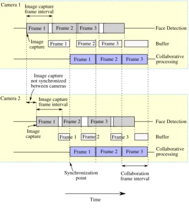
It is well known that synchronous distributed systems are in general less complex and, for some network types, more efficient than asynchronous systems [52]. Since synchronizing the time clocks of camera nodes interconnected by a local area network is relatively simple, we chose to employ a synchronous approach for our distributed camera network system. In our system, camera clocks are synchronized using the Network Time Protocol (NTP). Moreover, we assume that all the cameras in the network have a consistent frame capturing rate. However, even when that is true, it is not simple to synchronize the image capture times without using special hardware. That is, it is difficult to guarantee that the time instant at which the different cameras capture their frames will be exactly the same for all cameras. To overcome this problem, we designed a buffering mechanism that allows the cameras to store the current detections until they reach a synchronization point. The buffering mechanism is illustrated in Figure 8. As the cameras acquire the initial frame, they store the information in the buffer until they reach a synchronization point. At this point, collaborative processing is initiated and
Face Detection Image capture Image capture frame interval Image capture Camera 1 Camera 2 Image capture not synchronized between cameras Image capture frame interval Collaborative processing Collaboration frame interval Frame 1 Frame 2 Frame 3
Frame 1 Frame 2 Frame 3
Frame 1 Frame 2 Frame 3
Frame 1 Frame 2 Frame 3
Frame 1 Frame 2 Frame 3 Frame 1 Frame 2 Frame 3
Buffer Face Detection Collaborative processing Buffer Synchronization point Time
Figure 8: Buffer mechanism for camera synchronization. Cam-era capture and face detection are executed asynchronously. The results are stored in a buffer which is processed syn-chronously during the collaboration frame intervals.
the cameras are allowed to share information. In subsequent frames, new synchronized collaboration frame intervals occur at a predefined rate that is common to all cameras. This works as long as face detection can be carried out in less than one frame interval. However, since face detection time is variable, it may occasionally take longer than one frame interval. In that case, the detections corresponding to that frame are discarded and a new frame is processed without detriment to the collaborative processing synchronization.
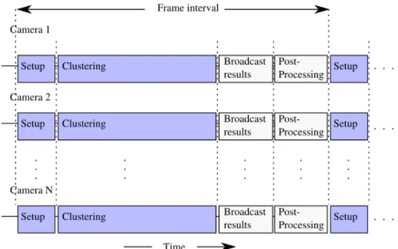
Figure 9 shows in detail the sequence of events that takes place during the collaboration intervals. During the brief setup step, all new clustering modules are initialized and prepared to receive messages from other cameras. This step provides tolerance for small errors in the synchronization of the cameras. Although not strictly necessary, this step greatly improves system efficiency by not having to buffer messages received by uninitialized clustering modules. At the beginning of the clustering step, the clustering protocol is executed and clusters are created, dissolved, or propagated as necessary. After the states of all the clusters are updated, the cluster members send their observations to the cluster leaders, which then integrate them into face pose estimates. After the clustering step, the cluster leaders update the estimate and prediction of the location of each face using a Kalman filter. The cluster leaders also broadcast the predicted face poses to the cluster members for association with the face detections in the next frame. To avoid the cluster switching from one person to another, if the cluster leader detects that the new
Figure 9: Collaboration interval steps. After a short setup period, all the cameras share information during the clustering step. Afterwards, cluster leaders broadcast the results to the cluster members, and post-processing algorithms may take place.
face pose estimate is far from the Kalman filter’s prediction, it terminates the cluster by sending a message to its members and deactivating itself. Finally, after the required processing is concluded, our system provides a time slot for the application of post-processing algorithms. In our current system, we use this slot to log the results of our experiments.
V. EXPERIMENTS
We implemented our algorithm on a network of twelve firewire cameras connected to three quad-core desktop com-puters. The cameras are arranged side-by-side in the form of a 2 ×6 array all facing approximately the same direction. Each camera has a separate process assigned to it. In each process, we manage the face position estimates and camera clustering assigned to that camera, and detect faces with a boosted classifier cascade [6], [45] trained using the FERET database [53]. Figure 10 shows four snapshots of the graphical user interface of our system. The top half of each snapshot shows a computer graphics representation of the 3D positions of the camera array, the clusters tracking the faces, and the estimated poses of the detected faces. Each camera is represented by a small cube and the face poses are indicated by a 3D face model [54]. The circles represent cluster leaders and the lines represent the members. A dashed circle or line indicates that the cluster leader or member did not contribute an observation for that particular frame. The bottom part of each snapshot shows the images captured by the cameras and the corresponding face detections as computed by the individual cameras.
Figure 11 shows qualitative results of one run of our experiments for one of the two people shown in Figure 10. The left column shows the 3D positions of the face, and the right column shows its orientation. In this figure, ground truth is represented by solid lines and the markers with different colors represent the estimated face poses. The reason for using different colors on the trajectories is to illustrate the moments
when the system loses track of a person’s face — each time the track is lost, a different color is used. Notice that when a cluster loses track, another cluster almost immediately is created and starts to track the face again.
In the experiments we present here, we require that all the cameras in a cluster detect a frontal face. A face can be accu-rately tracked if it is detected by at least two cameras. When the individual cameras have low detection rates, additional camera views can increase the likelihood of detecting the face. If non-frontal face poses can be localized in the individual images, fewer cameras will be needed by our protocol. Even when detecting only frontal faces, many camera configurations can be used with our current protocol. Because the clustering protocol allows for the propagation of the cluster, new cameras in different orientations can pick up the tracking of the face as the face rotates away from the old cameras.
A. Comparison with a Centralized Method
To provide a quantitative evaluation of our distributed ap-proach, we compare it to a centralized method which operates in a similar framework but does not include the clustering protocol.
The centralized version has many of the features of the dis-tributed approach. As in the disdis-tributed approach, we perform face detection locally in each camera. Thus face detection — which takes most of the processing time in our experiments — is still distributed in the centralized approach. The timing of both approaches is also similar. In both systems, we synchro-nize the processing of images as illustrated in Fig. 8. Despite these similarities, there are fundamental differences between the centralized and distributed versions. In the centralized version, no leader is elected. Instead, collaborative processing takes place in two steps. In the first step, every camera sends the observations to a single node for central processing. In the second step, the central node processes all the observations it received for that frame in batch.
Because all of the estimates are available in batch, we partition them into setsEl, l= 1, . . . , L, whereLis the number
of people in the environment, using an approximate clique clustering algorithm [55]. The sets are chosen to approximately minimize the sum of intra-set costs,
arg min L,El L X l=1 X pjw∈El,pkw∈El,pjw6=pkw cost(pjw,pkw) . (7)
This algorithm requires both positive and negative costs to produce non-trivial clusterings, so we use the cost function
cost(pjw,pkw) = d(pjw,pkw)−Tclique, where Tclique
deter-mines the zero-cost distance, andd(·)is given in Eq. (4). Figure 12 shows a comparison between the centralized tracker and our distributed approach. The tracks shown in the figure correspond to thexcoordinates of the two faces shown in Figure 10. As in Figure 11, different colors illustrate the moments when the system loses track of a face. Since neither approach represents an ideal tracker, lost tracks occur in both. We record two kinds of tracking errors for our system. If a track is lost, and a new one is created to track a person, we call
Figure 10: Snapshot of our tracking results. Top figures: graphical representation of the camera array and estimated poses. Bottom figures: images captured by each camera and the detected faces. The two frames at the top illustrate the propagation of a cluster leader.
this an "extra track." If a tracker switches from one person to another, we call this a "track switch." Track switches are worse than extra tracks because they indicate that a single tracker tracks two people. They are also much more rare in both the centralized and distributed systems. In ten runs of the system, the centralized system required an average of3.6±0.2extra tracks per person and 0 track-switches, and the distributed system required2.2±0.7 extra tracks and 0.1 track switches. We also compare the centralized and distributed approaches based on the frame-by-frame tracking performance, as shown in Table I. In each frame, we associate each ground-truth to a single integrated face estimate, if there is an estimate within a specific matching distance. True-positives (T P) rep-resent ground-truth and integrated estimate pairs, while false-positives (F P) represent estimates which do not correspond to any ground-truth. Pairs are assigned starting with the closest ground-truth and estimates, so that it is possible for an estimate to be within the matching distance and still be considered an
F P. TheRM SEestimates are based on theT P pairs. These results show that the distributed approach achieves comparable performance to the centralized version.
VI. CONCLUSION
We have presented a completely distributed face tracking algorithm that estimates the 6-DOF poses of multiple faces in
Table I: Tracking performance on the two-person sequence. Testing is done on 50 frames, spaced ten frames apart. These results are averaged over five runs for each system, each using the same multi-camera video sequence.
T Pa F Pa rmse
T(cm) rmseR(◦)
Centralized 95 (95%) 12 (12%) 5.8 20.8 Distributed 94 (94%) 4 (4%) 6.1 18.7 a
percentages are per frame, per person
real time. Each camera individually computes the world pose of the faces based on their visual features. The observations of multiple cameras are integrated using a minimum variance estimator and tracked using a Kalman filter. A clustering protocol is responsible for dynamically creating groups of cameras that track a given face and for coordinating the distributed processing.
As our experimental results show, our algorithm performs as well as a centralized approach while presenting the well-known advantages of distributed systems: scalability and ro-bustness. Since the computational load is dynamically trans-ferred among processors as the people move in the field of view of the camera network, our algorithm can potentially handle an arbitrary number of faces and can be scaled to much larger networks. Also, since cluster leaders are dynamically elected and the clustering protocol is robust to system failures,
0 100 200 300 400 500 0 50 100 150 200 X (cm) frames 0 100 200 300 400 500 0 50 100 150 200 Y (cm) frames 0 100 200 300 400 500 0 50 100 150 200 Z (cm) frames 0 100 200 300 400 500 −40 −20 0 20 40 ψ (degrees) frames 0 100 200 300 400 500 −40 −20 0 20 40 φ (degrees) frames 0 100 200 300 400 500 −40 −20 0 20 40 θ (degrees) frames
Figure 11: Qualitative results of one experimental run of the distributed face tracker on one of two faces (the second face is omitted for clarity).
the algorithm does not rely on a single server to process the information, therefore avoiding a single point of failure.
One limitation of our current approach is the representation of rotations using yaw, pitch, and roll angles, which, as any representation of rotations inR3
, have discontinuities that must be handled as special cases. We currently restrict ourselves to representations in R3
to allow the use of standard techniques for transforming distributions between Euclidean spaces. In the future, we would like to extend our method to use quaternions, but this requires more sophisticated techniques to transform rotation estimates from a three-dimensional Euclidean space to a three-dimensional manifold in a four-dimensional space. Another aspect that requires consideration is that the min-imum variance estimator — Eqs. (5) and (6) — is based on the assumption that the camera observations are independent. Although this is generally a good approximation, when we transform the observations from the image space to the world space, we incorporate prior knowledge about the size of a person’s face. This introduces a bias in the world space which manifests itself as observations which are consistently closer to the camera which detects them, or farther away, depending on whether the person’s face is larger or smaller than expected.
0 50 100 150 200 250 300 350 400 450 500 0 50 100 150 200 X (cm) frames 0 50 100 150 200 250 300 350 400 450 500 0 50 100 150 200 X (cm) frames
Figure 12: Comparison of tracking in the distributed (top) and centralized (bottom) versions. Marker color indicates the ID assigned to each track. Both the centralized and the distributed approaches are approximate and track ID changes are visible in both approaches. The ground truth for each track is indicated by a black line which is sampled every10th frame.
Although we believe that most of this bias is removed in the integration of the observations from multiple cameras — and our experimental results support that claim — in the future we would like to carefully investigate the effects of this bias in the estimation of the positions of the faces.
One advantage of our approach is that while it does not require image-based tracking methods such as particle filters or mean-shift [56], [57], [58], it does provides a good framework for incorporating such trackers which operate independently on different camera images. These trackers would provide additional observations which could be used to keep track of the faces when the interval between face detections is large. When new face detections become available, they could be used to reduce the chance that the trackers drift off of the true face location.
ACKNOWLEDGMENTS
This work was sponsored by Olympus Corporation. The authors wish to thank Hidekazu Iwaki and Akio Kosaka for many helpful discussions.
REFERENCES
[1] R. Stiefelhagen, M. Finke, J. Yang, and A. Waibel, “From gaze to focus of attention,” in Proceedings of the International Conference on Visual Information and Information Systems. Springer, 1999, pp. 761–768. [2] K. Smith, S. Ba, D. Gatica-Perez, and J.-M. Odobez, “Tracking the
vi-sual focus of attention for a varying number of wandering people,” IEEE Transactions on Pattern Analysis and Machine Intelligence, vol. 30, no. 7, pp. 1212–1229, 2008.
[3] H. Rowley, S. Baluja, and T. Kanade, “Neural network based face detec-tion,” IEEE Transactions on Pattern Analysis and Machine Intelligence, vol. 20, no. 1, pp. 23–38, 1998.
[4] H. Schneiderman and T. Kanade, “A statistical method for 3D object detection applied to faces and cars,” in Proceedings of the IEEE Conference on Computer Vision and Pattern Recognition, 2000. [5] C. Huang, H. Ai, Y. Li, and S. Lao, “High-performance rotation invariant
multiview face detection,” IEEE Transactions on Pattern Analysis and Machine Intelligence, vol. 29, no. 4, pp. 671–686, 2007.
[6] P. Viola and M. Jones, “Robust real-time face detection,” International Journal of Computer Vision, vol. 57, no. 2, pp. 137–154, 2004. [7] E. Murphy-Chutorian and M. Trivedi, “Head pose estimation in
com-puter vision: A survey,” IEEE Transactions on Pattern Analysis and Machine Intelligence, vol. 31, no. 4, pp. 607–626, Apr. 2009. [8] L. Brown, Y. Tian, I. Center, and N. Hawthorne, “Comparative study
of coarse head pose estimation,” in Proceedings of the Workshop on Motion and Video Computing, 2002, pp. 125–130.
[9] L. Zhao, G. Pingali, and I. Carlbom, “Real-time head orientation estimation using neural networks,” in Proceedings of the International Conference on Image Processing, 2002.
[10] E. Murphy-Chutorian, A. Doshi, and M. Trivedi, “Head pose estimation for driver assistance systems: A robust algorithm and experimental eval-uation,” in Proceedings of the IEEE Intelligent Transportation Systems Conference, Sept 2007, pp. 709–714.
[11] B. Raytchev, I. Yoda, and K. Sakaue, “Head pose estimation by nonlinear manifold learning,” in Proceedings of the International Conference on Pattern Recognition, 2004.
[12] T. Cootes, G. Edwards, and C. Taylor, “Active appearance models,” IEEE Transactions on Pattern Analysis and Machine Intelligence, vol. 23, no. 6, p. 681, Jun. 2001.
[13] T. Maurer and C. von der Malsburg, “Tracking and learning graphs and pose on image sequences of faces,” in Proceedings of the IEEE International Conference on Automatic Face and Gesture Recognition, 1996, pp. 176–181.
[14] T. S. Jebara and A. Pentland, “Parametrized structure from motion for 3D adaptive feedback tracking of faces,” in Proceedings of the IEEE Conference on Computer Vision and Pattern Recognition, 1997, pp. 144– 150.
[15] A. Schödl, A. Haro, and I. Essa, “Head tracking using a textured polygonal model,” in Workshop on Perceptual User Interfaces, 1998, pp. 43–48.
[16] J. Heinzmann and A. Zelinsky, “3-D facial pose and gaze point estima-tion using a robust real-time tracking paradigm,” in Proceedings of the International Conference on Automatic Face and Gesture Recognition, 1998, pp. 142–147.
[17] D. Decarlo and D. Metaxas, “Optical flow constraints on deformable models with applications to face tracking,” International Journal of Computer Vision, vol. 38, no. 2, pp. 99–127, 2000.
[18] M. La Cascia, S. Sclaroff, and V. Athitsos, “Fast, Reliable Head Tracking under Varying Illumination: An Approach Based on Registration of Texture-Mapped 3D Models,” IEEE Transactions on Pattern Analysis and Machine Intelligence, pp. 322–336, 2000.
[19] J. Tu, T. Huang, and H. Tao, “Accurate head pose tracking in low resolution video,” in Proceedings of the IEEE International Conference on Automatic Face and Gesture Recognition, 2006.
[20] Z. Zhang, A. Scanlon, W. Yin, L. Yu, and P. L. Venetianer, “Video surveillance using a multi-camera tracking,” in Multi-Camera Networks: Principles and Applications, H. Aghajan and A. Cavallaro, Eds. Else-vier, 2009, ch. 18, pp. 435–456.
[21] S. Calderara, R. Cucchiara, R. Vezzani, and A. Prati, “Statistical pattern recognition for multi-camera detection, tracking, and trajectory analysis,” in Multi-Camera Networks: Principles and Applications, H. Aghajan and A. Cavallaro, Eds. Elsevier, 2009, ch. 16, pp. 389–414. [22] J. Wu and M. Trivedi, “A two-stage head pose estimation framework and evaluation,” Pattern Recognition, vol. 41, no. 3, pp. 1138–1158, 2008. [23] L. Morency, A. Rahimi, N. Checka, and T. Darrell, “Fast stereo-based
head tracking for interactive environments,” in Proceedings of the IEEE International Conference on Automatic Face and Gesture Recognition, 2002, pp. 390–395.
[24] S. Koterba, S. Baker, I. Matthews, C. Hu, J. Xiao, J. Cohn, and T. Kanade, “Multi-view AAM fitting and camera calibration,” Proceed-ings of the IEEE International Conference on Computer Vision, 2005. [25] M. Yasumoto, H. Hongo, H. Watanabe, and K. Yamamoto, “Face
direction estimation using multiple cameras for human computer in-teraction,” in Proceedings of the International Conference on Advances in Multimodal Interfaces – ICMI. Springer, 2000, pp. 222–229. [26] C. Chang, C. Wu, and H. Aghajan, “Pose and gaze estimation in
multi-camera networks for non-restrictive HCI,” in Proceedings of the IEEE International Workshop on HCI, vol. 4796. Springer, 2007, p. 128. [27] E. Murphy-Chutorian and M. Trivedi, “3D tracking and dynamic
analysis of human head movements and attentional targets,” Proceed-ings of the International Conference on Distributed Smart Cameras (ICDSC’08), 2008.
[28] H. Iwaki, G. Srivastava, A. Kosaka, J. Park, and A. Kak, “A novel evidence accumulation framework for robust multi-camera person de-tection,” in Proceedings of the ACM/IEEE International Conference on Distributed Smart Cameras, Sep. 2008, pp. 1–10.
[29] W. B. Heinzelman, A. P. Chandrakasan, and H. Balakrishnan, “An Application-Specific Protocol Architecture for Wireless Microsensor Networks,” IEEE Transactions on Wireless Communications, vol. 1, no. 4, pp. 660–670, Oct. 2002.
[30] S. Bandyopadhyay and E. Coyle, “An energy efficient hierarchical clustering algorithm for wireless sensor networks,” in Proc. IEEE INFOCOM, vol. 3, 2003, pp. 1713– 1723.
[31] O. Younis and S. Fahmy, “HEED: A hybrid, energy-efficient, distributed clustering approach for ad hoc sensor networks,” IEEE Transactions on Mobile Computing, vol. 3, no. 4, pp. 366–379, Oct.-Dec. 2004. [32] S. Soro and W. Heinzelman, “Prolonging the lifetime of wireless
sensor networks via unequal clustering,” in Proceeedings of the IEEE International Parallel and Distributed Processing Symposium, April 2005.
[33] C. Liu, J. Liu, J. Reich, P. Cheung, and F. Zhao, “Distributed group management for track initiation and maintenance in target localization applications,” in Proceedings of the IEEE International Workshop on Information Processing in Sensor Networks, Apr. 2003.
[34] W.-P. Chen, J. Hou, and L. Sha, “Dynamic clustering for acoustic target tracking in wireless sensor networks,” IEEE Transactions on Mobile Computing, vol. 3, no. 3, pp. 258–271, Jul. 2004.
[35] W. Zhang and G. Cao, “DCTC: Dynamic convoy tree-based collabo-ration for target tracking in sensor networks,” IEEE Transactions on Wireless Communications, vol. 3, no. 5, pp. 1689–1701, Sep. 2004. [36] Y.-C. Tseng, S.-P. Kuo, H.-W. Lee, and C.-F. Huang, “Location tracking
in a wireless sensor network by mobile agents and its data fusion strategies,” The Computer Journal, vol. 47, no. 4, pp. 448–460, Apr. 2004.
[37] X.-H. Kuang, R. Feng, and H.-H. Shao, “A lightweight target-tracking scheme using wireless sensor network,” Measurement Science and Technology, vol. 19, no. 2, p. 025104 (7pp), 2008.
[38] Q. Fang, F. Zhao, and L. Guibas, “Lightweight Sensing and Commu-nication Protocols for Target Enumeration and Aggregation,” in ACM Symp. on Mobile Ad Hoc Networking and Computing (MobiHoc), 2003, pp. 165 – 176.
[39] F. Bouhafs, M. Merabti, and H. Mokhtar, “Mobile event monitoring pro-tocol for wireless sensor networks,” in Proceedings of the International Conference on Advanced Information Networking and Applications Workshops, AINAW ’07, vol. 1, 2007, pp. 864–869.
[40] W. Yang, Z. Fu, J.-H. Kim, and M.-S. Park, “An adaptive dynamic cluster-based protocol for target tracking in wireless sensor networks,” in Joint 9th Asia-Pacific Web Conference Advances in Data and Web Management, APWeb 2007, and 8th International Conference on Web-Age Information Management, WAIM 2007, 2007, pp. 157–167. [41] S. Soro and W. Heinzelman, “On the coverage problem in
video-based wireless sensor networks,” in Proceedings of the International Conference on Broadband Networks, Oct. 2005, pp. 932–939 Vol. 2. [42] ——, “A survey of visual sensor networks,” Advances in Multimedia,
vol. 2009, pp. 1–21, 2009.
[43] H. Medeiros, J. Park, and A. Kak, “Distributed object tracking using a cluster-based kalman filter in wireless camera networks,” IEEE Journal of Selected Topics in Signal Processing, vol. 2, no. 4, pp. 448–463, Aug. 2008.
[44] Y. Tian, L. Brown, J. Connell, S. Pankanti, A. Hampapur, A. Senior, and R. Bolle, “Absolute head pose estimation from overhead wide-angle cameras,” in Proceedings of the IEEE International Workshop on Analysis and Modeling of Faces and Gestures, 2003.
[45] R. Lienhart and J. Maydt, “An extended set of Haar-like features for rapid object detection,” Proceedings of the IEEE International Conference on Image Processing, vol. 1, no. 1, pp. 900–903, Sep. 2002. [46] S. Julier and J. Uhlmann, “A new extension of the Kalman filter to nonlinear systems,” in Proceedings of the International Symposium on Aerospace/Defense Sensing, Simulation and Controls, vol. 3, 1997. [47] A. Sankaranarayanan and R. Chellappa, “Optimal multi-view fusion of
object locations,” in Proceedings of IEEE Workshop on Motion and Video Computing. Citeseer, Jan. 2008, pp. 1–8.
[48] H. Medeiros, J. Park, and A. Kak, “A light-weight event-driven protocol for sensor clustering in wireless camera networks,” Proceedings of the ACM/IEEE International Conference on Distributed Smart Cameras, vol. 2, no. 4, pp. 203–210, Sep. 2007.
[49] J. Kurose and K. Ross, Computer Networking: A Top-Down Approach Featuring the Internet, 3rd ed. Addison Wesley, 2005.
[50] W. Zhao, R. Chellappa, P. Phillips, and A. Rosenfeld, “Face recognition: A literature survey,” ACM Computing Surveys, vol. 35, no. 4, pp. 399– 458, 2003.
[51] Y. Sheikh, O. Javed, and M. Shah, “Object association across multiple cameras,” in Multi-Camera Networks: Principles and Applications, H. Aghajan and A. Cavallaro, Eds. Elsevier, 2009, ch. 17, pp. 415–434. [52] N. Lynch, Distributed Algorithms. Morgan Kaufmann, 1997. [53] P. Phillips, H. Wechsler, J. Huang, and P. Rauss, “The FERET database
and evaluation procedure for face-recognition algorithms,” Image and Vision Computing, vol. 16, no. 5, pp. 295–306, 1998.
[54] V. Blanz and T. Vetter, “A morphable model for the synthesis of 3D faces,” in Proceedings of the ACM SIGGRAPH Conference on Computer Graphics, 1999, pp. 187–194.
[55] V. Ferrari, T. Tuytelaars, and L. Van Gool, “Real-time affine region tracking and coplanar grouping,” in Proceedings of the IEEE Conference on Computer Vision and Pattern Recognition, vol. 2, 2001.
[56] D. Comaniciu and P. Meer, “Mean shift: a robust approach toward feature space analysis,” IEEE Transactions on Pattern Analysis and Machine Intelligence, vol. 24, no. 5, pp. 603–619, May 2002. [57] P. Perez, C. Hue, J. Vermaak, and M. Gangnet, “Color-based
proba-bilistic tracking,” European Conference on Computer Vision, vol. 1, pp. 661–675, 2002.
[58] K. Nummiaro, E. Koller-Meier, and L. V. Gool, “An adaptive color-based particle filter,” Image and Vision Computing, vol. 21, no. 1, pp. 99 – 110, Jan. 2003.
Josiah Yoder received the BS CompE degree from Rose-Hulman Institute of Technology in 2005. He is currently pursuing a PhD degree in the School of Electrical and Computer Engineering at Purdue University. His research interests include computer vision, machine learning, human-computer interac-tion, and distributed computing.
Henry Medeiros received the BE and MS degrees in Electrical Engineering from the Federal University of Technology, Parana, Brazil, in 2003 and 2005 respectively. He is currently pursuing his PhD degree in the School of Electrical and Computer Engi-neering at Purdue University. His current research interests include sensor networks, computer vision, and embedded systems.
Johnny Park received the B.S., M.S., and Ph.D. degrees from the School of Electrical and Computer Engineering, Purdue University, West Lafayette, IN, in 1998, 2000, and 2004, respectively. He was a Principal Research Scientist at Purdue University where he led a large research project on distributed camera networks. He is currently a Research Assis-tant Professor in the School of Electrical and Com-puter Engineering at Purdue University. His research interests span various topics in distributed sensor networks, computer graphics, computer vision and robotics.
Avinash C. Kak is a professor of electrical and com-puter engineering at Purdue University. His research and teaching include sensor networks, computer vision, robotics, and high-level computer languages. He is a coauthor of Principles of Computerized Tomographic Imaging, which was republished as a classic in applied mathematics by SIAM, and of Digital Picture Processing, which is also considered by many to be a classic in computer vision and image processing. His recent book Programming with Objects (John Wiley & Sons, 2003) is used by a number of leading universities as a text on object oriented programming. His latest book Scripting with Objects, also published by John Wiley, focuses on object-oriented scripting. These are two of the three books for an “Objects Trilogy” that he is creating. The last, expected to be finished sometime in 2010, will be titled Designing with Objects.