Efficient Domain Partitioning for Stencil-based Parallel Operators

(1)

for

Stencil-based Parallel Operators

Gaurav Saxena

Submitted in accordance with the requirements

for the degree of Doctor of Philosophy

The University of Leeds

School of Computing

(2)

(3)

has formed part of a jointly authored publication has been included. The contribution of the candidate and the other authors to this work has been explicitly indicated below. The candidate confirms that appropriate credit has been given within the thesis where reference has been made to the work of others.

Some parts of the work presented in Chapters 1, 4, 5 and 6 have been published in the following articles:

Saxena, G., Jimack, P.K. and Walkley, M.A., 2016, July. A Cache-aware Approach to Domain Decomposition for Stencil-based Codes. In High Performance Computing & Simulation (HPCS), 2016 International Conference on (pp. 875-885). IEEE.

Saxena, G., Jimack, P.K. and Walkley, M.A., 2017, December. A Cache-aware Approach to Adaptive Mesh Refinement in Parallel Stencil-based Solvers. InHigh Performance Com-puting and Communications; IEEE 15th International Conference on Smart City; IEEE 3rd International Conference on Data Science and Systems (HPCC/SmartCity/DSS), 2017 IEEE 19th International Conference on (pp. 364-371). IEEE.

Saxena, G., Jimack, P.K. and Walkley, M.A., 2018. A Quasi-cache-aware Model for Optimal Domain Partitioning in Parallel Geometric Multigrid. Concurrency and Computation: Practice and Experience, 30(9), p.e4328.

The above publications are primarily the work of the candidate.

This copy has been supplied on the understanding that it is copyright material and that no quotation from the thesis maybe published without proper acknowledgement.

(4)

(5)

It has always been my dream to become a good researcher and I could not have chosen a better path than to pursue this PhD as the first step to achieving this goal. In this long, tough and fruitful journey, it has been an absolute honour and pleasure to have worked under the super-vision of ProfessorPeter K. Jimack and Dr. Mark A. Walkley. Together, they form a perfect team. Besides being brilliant researchers, they are amazing human beings who make every effort to understand the needs and problems of the student. Though one’s imagination is unlimited, it is not possible for me to imagine better supervisors than them. From the bottom of my heart, I profusely thank them for their guidance, care and encouragement. Thank you for letting me pursue my dream and I really hope this journey blossoms into a life-long academic collaboration.

My heartfelt thanks toDr. Karim Djemamefor taking out the time for my yearly progress meetings and supplying some extremely interesting ideas. His constructive feedback has helped me to expand the scope of the future work outlined in this thesis. My thanks to Dr. Brandon Bennett for very timely approving the travel grants for conferences. From the day I walked in, Judi Drew has constantly helped me to adjust to the life of the department. The number of times she has helped me book tickets, register for conferences and forwarded changes in flight schedules, qualifies for a world-record. Thank you to Dr. Peter Bollada for all the interest-ing conversations from across the table. His pleasant personality, jovial nature and helpinterest-ing attitude is certainly contagious. Despite the deficiency of grey cells in my right brain, I have been able to enjoy many conversations with Dr. Thomas Ranner. Beyond doubt, he is an excellent academician and person. Many thanks to Mark Dixon for the constant support he offered regarding the hardware and software on ARC2/ARC3. His knowledge of hardware is unparalleled. Thanks toMartin Callaghan for making all the training sessions extremely inter-esting. I am very grateful toAnn S. Almgren for taking out the time to meet me in the SIAM conference in Atlanta, US, to solve my doubts regarding BoxLib. Thanks toWeiqun Zhang for helping me understand some specific subroutines in BoxLib. Meng-Huo Chen (Alan) happily shared his PhD experience and wisdom with me whenever we had the time to look away from the screen. I really enjoyed these breaks. My thanks to all theanonymous reviewers for their time and suggestions which helped us to improve the work in this thesis. Many thanks tomy teachers at the University of Edinburgh who sparked my monotonically increasing interest in High Performance Computing. A big thanks to Dr. Sanjeev Singh and Dr. M. K. Das for helping and having faith in me in the worst of times. I am very grateful to Sanjay Batra sir, Dr. Harmeet Kaur,Dr. Baljeet Kaur,Negi sir,Anita maam,Dr. Manoj Aggarwal,Sanjay sir, Ajit ji,Amit ji,Bharat ji and Shakti ji for accepting me as a member of the HRC family. My stay at HansRaj college was one of the happiest times I ever had and it was because of you all.

(6)

human being I ever came across. My amazing friendSachin taught me the value of hard work and set an example on how to survive despite extreme adversities. Thanks to my good friend Anshu whose amazing sense of humour and spiritual knowledge is beyond this realm. Swap-nil Laxman Gaikwad has constantly shared, advised, helped and encouraged me in this tough journey and forever will I remain indebted to him. I profusely thank my super-amazing friends Rahul Arora, Divya Jain, Rashmi Shakya and Pranav Kumar Singh who have a golden heart and a hand that is always ready to help. I must thankSwapnil Sahu for his timely help and all the good times we shared. A super big thanks toKanika Malik for being a wonderful friend and making time to meet me every time I was about to start a new session at work. Thanks toJyoti Balwani for reminding me again and again that I am a good person. My wonderful childhood friend Vasuda Arora, who has been a constant source of support, deserves a big chunk of the thank-you cookie.

Little did I know that mygrandfather’s predictions about my education would turn out to be true. A big thanks to him for gifting my brother and me with a never-ending supply of books. I thank my supremely talented uncle who has always been an amazing friend to me. Love and thanks to mynephews for loving me even when I have not been able to do anything for them. A huge thanks to my sister-in-law for completing our family and making me feel at home during my visit. A big thanks to my brother for his intermittent yet excellent streams of advice and for easing my financial burdens. Mygrandmother forged my character and I am thankful to the universe that I was loved by the most noble soul ever to walk on earth. Thanks is a small word for myfather who stood like a rock in front of me when I needed him the most. Last and the most, I take this opportunity to thank mymother who was with me every step of this journey. If I have achieved anything in this life, it is because of her. I have not met anyone as learned and educated as her. Although she is too humble to accept but she has an honorary doctorate in a very rare subject called . . .Life.

(7)

(8)

(9)

Partial Differential Equations (PDEs) are used ubiquitously in modelling natural phenomena. It is generally not possible to obtain an analytical solution and hence they are commonly dis-cretized using schemes such as the Finite Difference Method (FDM) and the Finite Element Method (FEM), converting the continuous PDE to a discrete system of sparse algebraic equa-tions. The solution of this system can be approximated using iterative methods, which are better suited to many sparse systems than direct methods.

In this thesis we use the FDM to discretize linear, second order, Elliptic PDEs and consider parallel implementations of standard iterative solvers. The dominant paradigm in this field is distributed memory parallelism which requires the FDM grid to be partitioned across the available computational cores. The orthodox approach to domain partitioning aims to minimize only the communication volume and achieve perfect load-balance on each core. In this work, we re-examine and challenge this traditional method of domain partitioning and show that for well load-balanced problems, minimizing only the communication volume is insufficient for obtaining optimal domain partitions. To this effect we create a high-level, quasi-cache-aware mathematical model that quantifies cache-misses at the sub-domain level and minimizes them to obtain families of high performing domain decompositions. To our knowledge this is the first work that optimizes domain partitioning by analyzing cache misses, establishing a relationship between cache-misses and domain partitioning.

To place our model in its true context, we identify and qualitatively examine multiple other factors such as the Least Recently Used policy, Cache Line Utilization and Vectorization, that influence the choice of optimal sub-domain dimensions. Since the convergence rate of point iterative methods, such as Jacobi, for uniform meshes is not acceptable at a high mesh res-olution, we extend the model to Parallel Geometric Multigrid (GMG). GMG is a multilevel, iterative, optimal algorithm for numerically solving Elliptic PDEs. Adaptive Mesh Refinement (AMR) is another multilevel technique that allows local refinement of a global mesh based on parameters such as error estimates or geometric importance. We study a massively parallel, multiphysics, multi-resolution AMR framework called BoxLib, and implement and discuss our model on single level and adaptively refined meshes, respectively.

We conclude that “close to 2-D” partitions are optimal for stencil-based codes on structured 3-D domains and that it is necessary to optimize for both minimizing cache-misses and com-munication. We advise that in light of the evolving hardware-software ecosystem, there is an imperative need to re-examine conventional domain partitioning strategies.

(10)

(11)

List of Figures

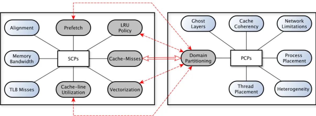
1.1 Serial Control Parameters (SCPs) Vs Parallel Control Parameters (PCPs): Our

focus is on Cache-misses and Domain Partitioning . . . 3

1.2 Macroscopic view of our research, grey boxes and red arrows show area of focus, FDM (Finite Difference Methods), FVM (Finite Volume Methods) and FEM (Finite Element Methods) are discretizations schemes, PARAMESH [1], Chombo [2], Uintah [3] and BoxLib [4] are parallel Adaptive Mesh Refinement (AMR) frameworks . . . 4

2.1 Finite Element unstructured mesh covering a square 2-D domain . . . 13

2.2 Common stencils in 2-D . . . 16

2.3 Common Stencils in 3-D . . . 16

2.4 DefaultMPI DIMS CREATE()algorithm used by OpenMPI . . . 30

2.5 Typical memory hierarchy with size and access times in a server system (repro-duced from [5]) . . . 40

3.1 Symmetric Multiprocessor (SMP) or Uniform Memory Access (UMA) multipro-cessor, each processor or core has uniform latency to main memory and a shared cache. . . 48

3.2 Distributed Shared Memory (DSM) or Non-Uniform Memory Access (NUMA) architecture where the SMP’s can access the distributed shared memory through an interconnection network, non-local memory access is non-uniform . . . 49

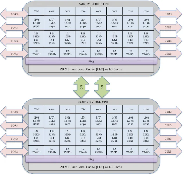
3.3 Memory hierarchy of an E5-2670 CPU processor and Quick Path Interconnect (QPI) . . . 50

4.1 A Vertex Centered (VC) problem of sizeNx×Ny= 5×5, having 4×4 internal mesh points is partitioned among 4 cores. The result is a (Px+ 2)×(Py+ 2) = (2 + 2)×(2 + 2) sub-domain with 4 original ’C’ cells and added ghost layer cells ’G’. . . 61

4.2 Domain decompositions corresponding to three virtual process topologies . . . . 62

4.3 Traditional optimization (solid arrows), our approach (dashed + solid arrows) . . 62

(18)

4.4 A 3-D sub-domain having an Independent Compute (IC) layer, Dependent Planes (DP) layer and Ghost/Halo layer, indexes of the sub-domain dimensions includ-ing the ghost layer are shown . . . 64 4.5 7-pt Stencil for updating the central red point . . . 65 4.6 A 7-point stencil in 3-D. The central point is updated according to prescribed

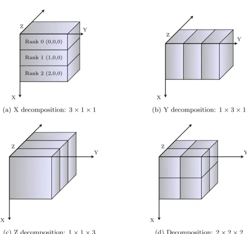
weights associated with, and values of the neighbouring points. . . 65 4.7 Process Grid Decomposition and Coordinate Axes (a) Shows process ranks in X

decomposition with MPI process coordinates (b) Only Y direction is decomposed (c) Only Z direction is decomposed (d) General decomposition in all 3 directions 66 4.8 Row-major and Column-major data layout . . . 67 4.9 High level iterative parallel PDE solver, e.g. Jacobi . . . 69 4.10 Unweighted Jacobi iteration kernel,alpha=constant, newandoldare 3-D data

arrays . . . 70 4.11 Dependent Z TOWARDS U (blue shaded vertical rectangle), adjacent points

distance (thick solid red line≈Pz) and boundary (unshaded circular points). . . 73

4.12 X-plane update: Data elements are contiguous (solid thick red line) except at boundary (dashed thick red line) . . . 76 4.13 Dependent Y LEFT plane (blue vertical shaded rectangle) and distance between

two adjacent points (solid red thick line). . . 77 4.14 Test problem illustration, Vertex centered, domainNx×Ny×Nz= 3×3×3,

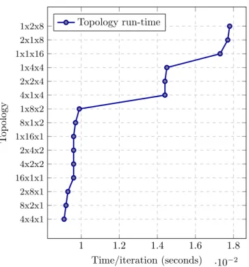
blue balls show Dirichlet boundaries and red balls show the unknowns . . . 81 4.15 Time/iteration Vs Topology for 16 processes (single SMP node of ARC2) on

problem size=2573_,_≈_{1048576 cells/process . . . 84}

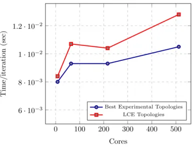
4.16 Time/iteration Vs Topology for 16 processes (single SMP node of ARC2) and varying problem sizes . . . 86 4.17 Weak Scaling for 8, 64, 216, 512 cores, Cells/core≈106_{, Iterations=10000, LCE}

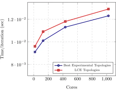
(Least Communication Elements), best topologies (4×2×1, 16×4×1, 6×12×3 and 8×32×2) Vs (2×2×2, 4×4×4, 6×6×6 and 8×8×8), respectively. . 90 4.18 Weak Scaling for 16, 128, 432, 1024 cores, Cells/core=1048576, Iterations=10000,

LCE (Least Communication Elements), best topologies (4×4×1, 16×8×1, 12×12×3, and 16×32×2) Vs (4×2×2, 8×4×4, 12×6×6, and 16×8×8), respectively. . . 92 4.19 Topology Timings for two runs of Problem Size=10253_{, P=1024 . . . 94}

4.20 Non-equivalence of tiled sub-domain and multiple sub-domains . . . 96 4.21 Cores in socket 0: blue balls, Cores in socket 1: red balls, Z-planes: very thick,

red lines, Y-planes: thick, black, dashed lines, X-planes: thin, blue, dotted lines, Decomposition: 2×2×2, QPI present on lines that connect different sockets, Mapping: --bind-to-core --bysocket . . . 98

(19)

4.22 Average time taken to send X, Y and Z planes of same size with cores=8 (topology=2×2×2) . . . 99 4.23 Average time taken to send X, Y and Z planes of same size with cores=64

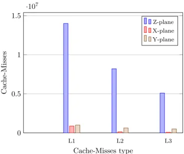
(topology=4×4×4) . . . 101 4.24 Cache-Misses for updating solution of Z/X/Y planes of equal sizes with Cores

P = 64, planes of size 64×64×4 bytes . . . 102 4.25 Cache-Misses for updating solution of Z/X/Y planes of equal sizes with Cores

P = 64, planes of size 128×128×4 bytes . . . 102 4.26 Topology Timings for 64 cores, Problem Size=401×401×401, Iterations=10000,

Cells/core≈106 for varying Memory Bandwidth per core . . . 103 4.27 19-pt stencil used in unweighted Jacobi,newandoldare 3-D data arrays . . . . 104 4.28 Time per iteration (seconds) of topologies using a 19-pt stencil whenP = 16 with

varying data sizes on a single node of ARC2, Intel compiler 17.0.1, Optimization level: -O2, OpenMPI 1.6.5 . . . 106 4.29 Time per iteration of various topologies using a 19-pt stencil with P = 64 and

N = 401×401×401, Intel compiler 17.0.1, OpenMPI 1.6.5 . . . 107 4.30 Example of an Irregular cut on a square domain that divides the domain into

two sub-domains s1 and s2 which do not have identical shape . . . 109 4.31 Weighted Jacobi (ω-Jacobi) iteration kernel, alpha=constant, newandold are

3-D data arrays . . . 111 4.32 Gauss-Seidel iteration kernel,alpha=constant,newis a 3-D data array . . . 112 5.1 Plots fory= tanh(k(x−0.5)) on a domain [0,1] withk= 5, 10, 20 and 30 . . . . 120 5.2 Domain [0,1]×[0,1] divided into 4 blocks having 16×16 cells each, grid spacing

h= 1

32 . . . 121

5.3 Refinement levels (Rfl) for obtaining increased precision for the PDE ∇2_u₌_f

having solutionu= tanh(k(x−0.5)) by refining in the region 0.45< x <0.55 . . 122 5.4 Refinement levels (Rfl) for a mesh when the region 0.8< x2₊_y2_<₀_._{9 is refined}

using blocks of size 8×8 . . . 123 5.5 Relationship between a Box, Fab, BoxArray, layout and MultiFab. The labels 1

and N are the cardinality of the relationship named “Contains”. . . 124 5.6 Cell centered and nodal data in BoxLib . . . 125 5.7 Fabs and MPI Cartesian Topology Rank numbering in 2-D . . . 126 5.8 16 Fabs (or boxes) spread on 4 processes arranged as 2×2. Each color shows a

single MPI process and numbers inside circles show the Fab number . . . 128 5.9 Varying box sizes with Domain = 16×16, 4 processes (arranged as 2×2), and

4 boxes per sub-domain . . . 130 5.10 Sub-domain shapes/sizes resulting from two of several MPI Cartesian Topologies

(20)

5.11 2-D slices of a 3-D domain having 243_{cells at}_x_{= 0}_._5,_y_{= 0}_._{5 and}_z_{= 0}_.₅

show-ing evolution of the numerical solution for ∇2_u _{= 0 with Dirichlet boundaries}

set to 1 at iteration count 0 and 800 . . . 140

5.12 Number of topologies outperforming the default mpi dims create() and Rev. mpi dims create()topology at various domain sizes and number of cores . . . . 141

5.13 Percentage gain of the best topology over MDC and Rev. MDC for varying domain sizes and cores . . . 143

5.14 L1d and L2d cache-misses for domain=483_{for the Compute kernel (C),} Commu-nication (Comm) and Boundary update (Bndry) . . . 144

5.15 L1d and L2d cache-misses for domain=963for the Compute kernel (C), Commu-nication (Comm) and Boundary update (Bndry) . . . 144

5.16 L1d and L2d cache-misses for domain=3843 _{for the Compute kernel (C),} Com-munication (Comm) and Boundary update (Bndry) . . . 145

5.17 Initial guess of zero to the final solution for 2 levels of a 163_{domain for our AMR} test problem . . . 146

5.18 Strong Scaling (time/iteration) two AMR levels problem with boxes of vary-ing shapes but equal volume usvary-ing Intel compilers 17.0.1 and OpenMPI 2.0.2, Optimization flags: -O3 -xHost -ip -align array64byte . . . 147

5.19 Strong Scaling (time/iteration) three AMR levels problem with coarsest grid being 5123 and boxes of varying shapes but equal volume using Intel compil-ers 17.0.1, Intel MPI 2017.1.132, OpenMPI 2.0.2 and Optimization flags: -O3 -xHost -ip -align array64byte . . . 148

6.1 Decreasing mesh resolution with decreasing level in 2-D Geometric Multigrid . . 156

6.2 Full 27-point restriction weights in 3-D for the central point (red) . . . 159

6.3 V-cycle in Multigrid . . . 161

6.4 Multigrid Algorithmvh_←_{M G}₍_vh_{, f}h_{) . . . 161}

6.5 Dirichlet-Neumann mixed Boundary Value Problem . . . 164

6.6 Front 2-D view of nine data-streams indicated by a ‘D’ in a 27-pt stencil in 3-D, dotted lines and arrows show direction in which data is contiguous . . . 169

6.7 Factors affecting selection of sub-domain dimensions . . . 174

6.8 Weak Scaling Independent Compute (IC) for P=1,2,4,8 and 16 processes with 643 16, 1283 16 , 2563 16 and 5123 16 cells per core (with no communication) to measure impact of shared Last Level Cache per-socket contention on execution times on ARC2 . . . 178

6.9 Baseline/naive implementation, Compiler optimized run-times with-O3 -xHOST -ip -ansi-alias -fno-alias, Heuristic square tile for X/Y dimensions (based on Rivera and Tseng [6] square tiles), Exhaustive Tiling for domain of size 5123 and 16 processes on ARC2, defaultMPI Dims create()= 4×2×2 . . . 182

(21)

6.10 Maximum average time (maximum time over processes and average of runs) to send and receive X/Y/Z planes separately within a 16-core node for topologies (--bind-to-core -bysocket) using Intel 16.0.2 and OpenMPI 1.6.5 on ARC2, defaultMPI Dims create()= 4×2×2 . . . 185 6.11 Maximum average time (maximum time over processes and average of runs) to

send and receive X/Y/Z planes separately within a 16-core node for topologies ((--bind-to-core -bycore)) . . . 186 6.12 Relative plane communication and Independent computation times for N = 64

andN = 128 withP= 16 ((--bind-to-core -bysocket)) using Intel 16.0.2 and OpenMPI 1.6.5 on ARC2, plane update execution times are not shown, default MPI Dims create()= 4×2×2 . . . 187 6.13 Intranode execution times of Parallel Geometric Multigrid using Baseline (Base),

aggressive Compiler Optimization (CO) and Heuristically Tiled (HT) versions on ARC2 and ARC3 . . . 189 6.14 16 processes in a single node of ARC2 arranged by--bind-to-core -bysocket,

Blue squares represent socket 1, Red balls represent socket 2, thick black lines are Z-planes, thick blue lines are X-planes, thick red lines are Y-planes. . . 190 6.15 Topology Run-times forP = 24,N = 576, Levels = 5, Coarsest iterations = 400,

5 V(3,3) cycles and the minimum run times for various combinations of compilers and MPI implementations on ARC3, defaultMPI Dims create()= 4×3×2 . . 192 6.16 Execution times of Geometric Multigrid for P = 64, Fine Grid = 5123_{, Levels}

= 6, Global Coarsest Grid = 163, ν1=ν2= 3, Fixed Coarsest iterations = 100,

Vcycles = 5, Intel 16.0.2, OpenMPI 1.6.5, ARC2, defaultMPI Dims create()= 4×4×4 . . . 194 6.17 P = 64, Fine Grid = 5123_{, Levels = 6, Global Coarsest Grid = 16}3_, _ν

1 =ν2 =

3, Fixed Coarsest iterations = 100, Vcycles = 5, Intel 16.0.2, OpenMPI 1.6.5, ARC2, defaultMPI Dims create()= 4×4×4 . . . 195 6.18 Total run-time and Fine Grid smooth-times for P = 512, Fine Grid = 10243_,

Levels = 6, Global Coarsest Grid = 323_,_ν

1=ν2= 3, Fixed Coarsest iterations =

800, Vcycles = 5, Intel 16.0.2, OpenMPI 1.6.5, ARC2, defaultMPI Dims create() = 8×8×8 . . . 197 6.19 Baseline (Base), Compiler Optimized (CO), Heuristically Tiled (HT) and HT

+ Explicit Vectorization (Vec) total run-time of topologies with Intel 17.0.1, OpenMPI 2.0.2 on ARC3 . . . 199 6.20 Topology Run-times forP = 24,N = 576, Levels = 5, Coarsest iterations = 400,

5 V(3,3) cycles for various combinations of compilers and MPI implementations on ARC3 using a 19-pt stencil in the smoother, default MPI Dims create() = 4×3×2 . . . 203

(22)

6.21 19-pt Smoother in Multigrid, Cores=96, N=768, Levels=5, Coarsest iterations=800, 5 V(3,3) cycles, Intel Compiler 17.0.1, OpenMPI 2.0.2 . . . 205 6.22 Prediction classes for representative cases of model accuracy on ARC3, where

(23)

List of Tables

3.1 ARC2 Features: Core, Processor and Node characteristics [7] . . . 52 3.2 ARC3 Features: Core, Processor and Node characteristics (standard nodes only) 53

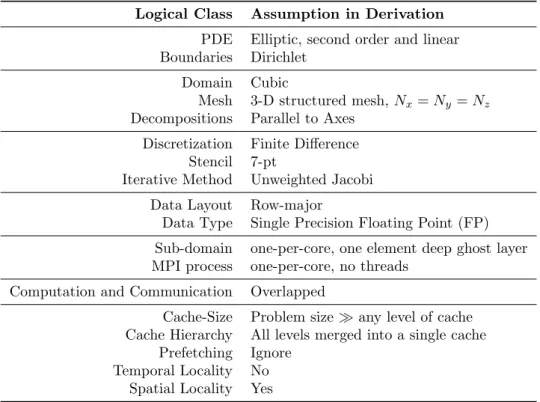
4.1 Model Assumptions: Logically classified assumptions in deriving the model . . . 70 4.2 Z-Plane: Relevant parameters for Z-plane showing total size, distance between

two adjacent elements, cache-misses in packing (reading)/unpacking (writing) and updating an element amongst others. . . 75 4.3 X-Plane: Relevant parameters for the X-plane showing total size, the maximum

gap between two adjacent elements, read/write cache-misses in packing/unpack-ing and update . . . 75 4.4 Y-Plane: Relevant parameters for the Y-plane including its size, maximum gap

between two adjacent elements, read/write misses in packing/update. . . 76 4.5 Independent Compute (IC): Relevant parameters including the size, maximum

gap between two elements, and read/write cache-misses in update. . . 78 4.6 Plane Cache-Misses: read/write cache-misses in packing/unpacking/updating X,

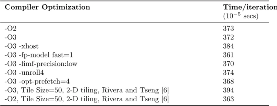
Y and Z-planes . . . 79 4.7 Optimizations: Time per iteration with different compiler options for problem

size=161×161×161 and cores=16 . . . 87 4.8 Compiler Options: Brief explanation of various compiler options for the Intel

C/C++ compiler . . . 87 4.9 Predicted and Actual cache-misses: Predicted Cache-Misses (PCM) and Actual

cache-misses for Problem Size=161×161×161, Cores=16, Iterations=19353, Independent Compute Elements (ICE)=199712, PCM for ICE=62410 . . . 88 4.10 Strong Scaling I: Strong Scaling for problem size=5133_{, Iterations=500,}_t

Best is

the minimum execution time,tM DC is the execution time of default MDC . . . . 93 4.11 Strong Scaling II: Strong scaling for problem size=10253_{, Iterations=500,}_t

Best

is the minimum execution time,tM DC is the execution time of default MDC . . . 93 4.12 Non-overlapped cache-misses: Cache read/write misses for the X, Y and Z planes

when computation is not overlapped with communication . . . 115

(24)

5.1 Set-up Variables: Declared variables during Set-up phase . . . 134 5.2 Uniform Grid: mpi dims create() (MDC)topology execution times per iteration

as compared to best topology times and reverse MDC. #MDC and #Rev. MDC gives the number of topologies performing better than MDC and Rev. MDC, respectively. No Loop blocking/Tiling was used, Intel compiler 17.0.1, OpenMPI 2.0.2 . . . 142 5.3 AMR: Gain percentage for the best performing topology over MDC for various

core counts, MDC=Solve time/iteration in seconds, Best=Best solve time/iteration147 5.4 Macroscopic view: Total L1, L2 and L3 cache-misses in the AMR application

with 2 levels, domain=5123 _{with box-sizes 128}_×₁₂₈_×_{128 and 256}_×₁₂₈_×_{64 . 149}

5.5 Cache-Misses Subroutines: Major sources of cache-misses for a 2 level AMR with domain=5123_{, block-sizes=128}_×₁₂₈_×_{128 and 256}_×₁₂₈_×_{64 . . . 150}

6.1 Interpolation: operator in 2-D . . . 159 6.2 Trilinear Interpolation: operator in 3-D . . . 160 6.3 Predicted Cache-Misses: Cache read/write/update misses for the dependent X,

Y and Z-plane . . . 167 6.4 Trade-off: Theoretical Communication Volume Vs Predicted Z-plane Cache-Misses174 6.5 h-independence: of Parallel Geometric Multigrid, Coarsest Grid tolerance =

10−8_{, Finest Grid tolerance = 10}−5 _{. . . 188}

6.6 Plane Types: Categories of planes based on network elements that they pass through, namely, node/shelf/rack . . . 196 6.7 Plane Frequency: Number of X/Y/Z Intranode/Intra-shelf/Intra-rack planes for

1-D topologies on ARC2 . . . 196 6.8 Extreme topologies: Run-times for N = 5123_, _P _{= 64, GCG = 64}3_{, Coarsest}

iterations = 100, Vcycles = 5,ν1=ν2= 3, ω= 1, FG (Fine Grid), CG (Coarsest

Grid), Intel 16.0.2, OpenMPI 1.6.5, ARC2 . . . 196 6.9 Weak Scaling Design Experiment: Fixed 2 V(3,3) cycles, 717 coarsest grid

iter-ations for first V-cycle and 712 coarsest grid iteriter-ations for second V-cycle . . . . 198 6.10 Weak Scaling on ARC2: Highest performing Vs standard topology percentage

performance gain, Intel 16.0.2, OpenMPI 1.6.5 . . . 200 6.11 Weak Scaling on ARC3: Highest performing Vs standard topology percentage

performance gain, TR (Total Run-time), FG (Fine Grid), Base (Baseline), CO (Compiler Optimized), HT (Heuristically Tiled), Vec (explicit Vectorization), Intel 17.0.1, OpenMPI 2.0.2, Coarsest iterations = 200,≈18 million cells/core, Global Coarsest Grid = 483 _{. . . 201}

6.12 Strong Scaling on ARC2: % performance gain of Cache Minimizing Topology over Standard Topology for Baseline, Compiler Optimized and Heuristically Tiled versions, N=512, 20 V(3,3) cycles, Coarsest iterations = 100, Levels = 6, Intel 16.0.2, OpenMPI 1.6.5 . . . 201

(25)

6.13 Strong Scaling on ARC3: % performance gain of Cache Minimizing Topology over Standard Topology for Baseline, Compiler Optimized and Heuristically Tiled with Explicit Vectorization versions, N=768, 5 V(3,3) cycles, Coarsest iterations = 400, Levels = 6, Intel 17.0.1, OpenMPI 2.0.2 . . . 201 6.14 Best Topologies and Percentage Gains: Best topologies for Base (Baseline), CO

(Compiler Optimized), HT (Heuristically Tiled) versions and percentage gain over the default MDC on a single node of ARC3 for N=576, 5 V(3,3), Levels = 5, Coarsest iterations = 400, 19-pt Parallel Geometric Multigrid . . . 204 6.15 Model Accuracy: _P = number of cores, _N = Domain size, np = Number of

predicted topologies, _fnp = Predicted topologies for whichtp< tM DC, _MDC= MPI Dims create()topology, Accuracy (True +) = npf

np ×100 . . . 206

(26)

(27)

Chapter 1

Introduction

With the stagnation of processor speeds [5], the delivery of continued computational perfor-mance improvements over the coming years will be through the exploitation of multicore proces-sors. In the post-Moore [5] era, where researchers are exhaustively hunting for performance in the hardware-software ecosystem, sequential is no longer tolerable. Hence, to quench the thirst for performance, the world is going parallel. The wide heterogeneity in multicore architectures, for example Manycore, Graphics Processing Units (GPUs) and the Field-Programmable Gate Arrays (FPGAs) to name a few, has already created a requirement for performance porta-bility. Irrespective of the multitude of architectures, the fundamental way in which problems are decomposed and distributed onto these parallel machines has not changed. Functional de-composition perceives work to be made up of a set of functions that need to be mapped onto multicores whereasDomain decomposition or Domain partitioningdivides the largest shareable data-structures among cooperating processes with the universal aim to minimize the commu-nicated volume of data between them.

Scientific Computing employs mathematical techniques to model, simulate and understand physical phenomena on modern computer systems. Undeniably, one of the most important mathematical tools to model phenomena occurring in nature is that of Partial Differential Equations (PDEs). In order to approximate such models on computers, it is necessary to map from a continuous domain to a domain represented by a finite set of points or elements spanning the original domain. Such discretizations are subsequently utilized by numerical al-gorithms to produce an approximated solution to the actual/analytical solution. Parallelism, being pervasive, has heavily influenced the field of Scientific Computing as well, leading to a well documented increase of performance over the years. There is thus an imperative need to continue this quest for computational speed by integrating state of the art techniques of Parallel Computing into Scientific Computing.

(28)

PDEs are generally classified asElliptic, Parabolic or Hyperbolic and their solution can be numerically approximated after a suitable discretization has been chosen. A well known method for discretization is theFinite Difference Method (FDM) that approximates the derivatives in the PDE using finite differences. Using the FDM on regular domains (e.g. rectangular or hexahedral) leads to the creation of a mesh or grid, where the solution at a particular point is expressed in terms of the weighted average of the solution at some fixed number of neighbouring points. Thus, emerges a fixed geometrical pattern called aStencil which, when coupled with a numerical iterative method, systematically updates the solution at each mesh point. These pat-terns when implemented on modern computer systems using standard data structures such as arrays, access non-contiguous as well as contiguous memory locations. It is this access pattern of stencil-codes that necessitates an optimal utilization of thecache-memory hierarchy as their performance is bounded by the memory bandwidth andlatency. Further, it is this very access pattern that motivates us to re-examine the fundamental approach of domain partitioning in parallel settings. Our research thus investigates a novel approach of domain partitioning for stencil-based parallel operators and in the process, challenges the orthodox approach of simply minimizing communication volume during domain partitioning.

Traditionally and universally, for load-balanced applications, domain partitioning has been a function of communication volume only. Thus, the aim of this approach has been to obtain equal-sized partitions that minimize the communication volume exchanged between the sub-domains. To the best of our knowledge, there is no literature on investigating the effect of cache-misses on domain partitioning. This is the very topic of this thesis, where we take the first step in connecting a pureSerial Control Parameter (i.e. cache-misses) to a pureParallel Control Parameter (i.e. Domain Partitioning). To this effect we build a high level mathemat-ical model to quantify/minimize cache-misses and obtain families of high performance domain partitions. For the remainder of this Chapter we aim to provide an overview of the focus of our research, while leaving the details to the chapters that follow.

1.1 Our Focus

Overheads in the form of communication, load-imbalance, limited memory-bandwidth, im-balance between processor and memory speeds, network and memory latencies, and complex memory hierarchies necessitate careful optimization of memory-bandwidth-limited stencil-based codes [8–15]. These overheads can be broadly classified as serial overheads or parallel overheads. Serial overheads, i.e. overheads which would still be present in the absence of multicore architec-tures, can be differentiated from parallel overheads (overheads which come into existence only because of the utilization of multicores). For example, cache-misses, TLB (Translation Looka-side Buffer) misses and memory latencies are examples of serial overheads which, along with

(29)

Figure 1.1: Serial Control Parameters (SCPs) Vs Parallel Control Parameters (PCPs): Our focus is on Cache-misses and Domain Partitioning

serial optimizations such as Vectorization, memory alignment etc., we shall collectively refer to asSerial Control Parameters (SCPs). Core-to-core latencies, network bandwidth/latencies, non-optimal process placement, non-optimal domain partitions and cache coherence conflicts in shared caches are examples of parallel overheads - a category which, along with the techniques to optimize them, we shall refer to as Parallel Control Parameters (PCPs). Figure 1.1 shows some SCPs and PCPs. Our focus is shown with the help of red arrows and grey boxes in Figure 1.1.

More research has explored SCPs as compared to PCPs, whilst there is a complex interac-tion of SCPs and PCPs which has little literature. Our research focus is to investigate this very interaction but due to the large interaction space between SCPs and PCPs, we restrict ourselves to the most important SCP which we practically (and from the literature [12–14, 16–18]) iden-tify to be Cache-misses and Domain Partitioning - the first fundamental step in distributing data on multicores. We thus take the first step in connecting Cache-misses to Domain Parti-tioning for single level and multilevel numerical algorithms on structured 3-D domains resulting from finite difference discretizations of Elliptic PDEs. Though applied only to finite difference discretizations of Elliptic PDEs, we argue that our conclusions can be extended to other prob-lems, such as implicit solution of Parabolic PDEs, finite element discretizations using trilinear elements on structured 3-D grids, or any other application that utilizes the same data access and communication pattern as that for the stencil-based codes under study. While construct-ing a mathematical model to establish this relation, we inherently assume that communication is overlapped with computation but argue that, with appropriate quantitative differences, the model can be applied to scenarios where there is no overlapping.

(30)

nu-Figure 1.2: Macroscopic view of our research, grey boxes and red arrows show area of focus, FDM (Finite Difference Methods), FVM (Finite Volume Methods) and FEM (Finite Element Methods) are discretizations schemes, PARAMESH [1], Chombo [2], Uintah [3] and BoxLib [4] are parallel Adaptive Mesh Refinement (AMR) frameworks

merically solve PDEs, we also test our hypothesis in adaptively refined meshes implemented in a library called BoxLib [19]. Adaptive Mesh Refinement (AMR) is a technique that allows a mesh to be refined locally depending on regions of estimated high error, geometric importance or some other parameter. It is an invaluable technique used in Scientific Computing and a key application targeted forExascale Computing [20]. BoxLib is a parallel framework that supports massive, multiscale, multiphysics problems and is written in a combination of C++/Fortran90. We discuss the challenges and the partial success of our model when evaluated in the environ-ment offered by BoxLib. After evaluating our model on adaptive meshes, we then extend the model developed to parallelGeometric Multigrid (GMG) - an optimalO(N) solution algorithm that is based on a hierarchy of grids of decreasing resolution. GMG is one of the most im-portant components of scalable numerical algorithms for solving Elliptic PDEs and is again an extremely important candidate for Exascale systems.

Figure 1.2 shows a macroscopic view of our research, with the area of focus being shown with the help of grey boxes and red arrows. We discretize Elliptic PDEs using Finite Difference Methods (FDMs) (as opposed to Finite Element (FEM) or Finite Volume (FVM) methods) and then use iterative methods (as opposed to direct methods) to solve the PDE on structured regular and adaptively refined meshes. Further, we use Geometric Multigrid for solving the discretized Elliptic PDE. In all the aforementioned scenarios, our aim is to compare the per-formance of sub-domains derived from our model against traditional communication volume minimizing partitions in parallel settings.

Further, we seek to present our model in the context of all the factors that might influence the choice of sub-domain shape and size. Thus, we qualitatively and quantitatively consider factors such as cache-misses, prefetching, cache-eviction policy, Vectorization etc. (see Figure 1.1), and explore their effect on determining optimal sub-domain dimensions. Though these

(31)

factors have been separately well explored in the literature, the focus of our work is on estab-lishing a connection between them and domain partitioning.

1.2 Thesis Contribution

In this section we summarize the main contributions that we claim for this thesis. We itemize these as follows.

– We take the first step in connecting the most important SCP of cache-misses to the fundamental PCP of Domain Partitioning for stencil-based codes. To the best of our knowledge, this relation/dependence has not been explored in the literature. We achieve this by building a high level, abstract, quasi-cache aware mathematical model to mini-mize the cache-misses and obtain families of high performing domain partitions. In this process, we question and challenge the orthodox approach of domain partitioning (for load-balanced codes) based on communication volume only and design experiments to evaluate the same.

– We take a step further to qualitatively establish the effect of other SCPs such as cache-eviction policy, Vectorization etc., on optimal sub-domain dimensions.

– As the model above is constructed using single level meshes, we extend it to multiple levels and evaluate its efficacy on parallel Geometric Multigrid.

– We show that the cache-miss equations for a 7-pt, 19-pt and 27-pt stencil in 3-D have the same form but with appropriate quantitative differences.

– We demonstrate hardware-software independence of our model since the only factor in-fluencing it is the data-layout in memory which is dependent on the language being used to implement the application.

– By implementing a Cartesian Topology for single level uniform meshes in BoxLib - an Adaptive Mesh Refinement framework supporting massively parallel, multiscale and mul-tiphysics problems - we are able to show experimentally the efficacy of our model even when communication is not overlapped with computation.

– We propose three dynamic, super-lightweight cache-tiling heuristics and evaluate the ef-ficacy of the simplest one of them in our experiments.

– We observe a partial success of our hypothesis when evaluating on adaptively refined meshes. This partial success is important as it shows the communication volume mini-mizing sub-domain shapes are not always the optimal even in load-imbalanced scenarios.

(32)

– Finally, we provide recommendations to application developers and (hopefully) theMPI Forumto re-examine and investigate the MPI Cartesian topology returned by the default MPI DIMS CREATE()function in the context of C (row-major layout) and Fortran (column-major layout) from a performance perspective.

1.3 Thesis Outline

Chapter 2 presents the necessary background along with a literature survey of the associated work. The ideology followed in this Chapter is to explore in depth the concepts which have been utilized in our work but also to span the breadth by broadly discussing associated research.

Chapter 3describes the hardware test platforms that we use for carrying out experiments, as well as broadly describing the software that we use for implementations and performance measurement. There are two major platforms that we use: ARC2 andARC3 - both resident at and managed by theUniversity of Leeds.

Chapter 4is dedicated to the development of our abstract, high level, mathematical model to obtain cache-minimizing domain partitions using single level, structured 3-D grids. We model the cache-misses by using the Jacobi iterative method used in approximating the solution of an Elliptic PDE discretized using the Finite Difference Method. Here, we specifically list our assumptions in creating this model and discuss their generalization to expand the model’s ap-plicability.

Chapter 5 evaluates the hypothesis formulated in the previous Chapter on uniform and adaptively refined meshes implemented using BoxLib. We further describe the challenges in adapting BoxLib while evaluating our model.

Chapter 6 is devoted to extending and evaluating the technique developed for single level meshes to parallel Geometric Multigrid, an acceleration convergence scheme that utilizes a hi-erarchy of grids of decreasing resolution. In addition to cache-misses, we qualitatively discuss how other SCPs affect optimal sub-domain dimensions.

Chapter 7 concludes the research presented in this thesis, discusses its successes and its limitations and presents ideas to open further research avenues.

(33)

Chapter 2

Background and Related work

This chapter provides the necessary background and an overview of the work related to the thesis. We start with a discussion of Partial Differential Equations (PDEs) since in the cur-rent work we focus onlinear, second order, Elliptic PDEs and their numerical solution using Iterative methods [21, 22]. PDEs are routinely used to model phenomena in Elasticity, Fluid Dynamics, Quantum Mechanics, Brownian Motion, Diffusion, Heat Transfer and Electrostatics, among many others [21, 23]. It would not be wrong to say that their numerical solution forms the backbone of Scientific Computing. PDE model problems involve continuous dependent variables defined on continuous domains but when their solution is approximated on computer systems, some form of discretization scheme is needed to describe the domain and the unknowns in terms of a finite number of values of a finite number of points or elements. There are many schemes for discretization such as Finite Difference Methods (FDM), Finite Element methods (FEM), Finite Volume Methods (FVM) and Spectral schemes, etc. We use the FDM in the current work and describe it in some detail. FEM is one of the most widely used schemes and is more flexible than FDM. After furnishing sufficient details, we very briefly touch upon some other discretization schemes. Finite difference discretization of Elliptic PDEs generally give rise to Sparse matrices, i.e. matrices which have very few non-zero entries as compared to entries which are zero. An associated concept is that of a Stencil - a fixed geometrical pattern used to update the solution on individual points of the domain using weighted contributions of the neighbouring points. We use the 7-pt, 19-pt and 27-pt stencils in 3-D in this work. The Sparse linear systems arising from FDM discretization of Elliptic PDEs can be solved using either Di-rect methods or Iterative methods. We describe theGaussian elimination direct method then move onto describing the iterative methods of Jacobi andGauss-Seidel in detail. Jacobi and weighted Jacobi iterative methods have been used in the current work to illustrate our research but the same can be extended to the Gauss-Seidel method and its variants.

Since we concentrate onDomain Partitioning in parallel settings, we describe various

(34)

els of carrying out parallel computing with an emphasis on the Message Passing Interface (MPI) [24]. The traditional method of domain partitioning universally revolves around mini-mizing the communication volume and we describe how the same is associated with the default MPI Cartesian Topology for structured domains. After describing the nature of sub-domains obtained after domain partitioning of structured 3-D domains, we discuss the opportunity that MPI provides for overlapping communication with computation for enhancing application per-formance. Performance metrics such asSpeed-up, Efficiency, Strong Scaling and Weak Scaling are discussed and used at appropriate points in experiments conducted for validating the con-cepts developed in the thesis.

Multigrid is a hierarchical, optimal, iterative solver for Elliptic PDEs which accelerates the convergence to the solution. Iterative solvers can thus be used on single grids or form a part of Multigrid [25] in the smoothing/solve phase. Our focus is on Geometric Multigrid (GMG)in parallel settings in the thesis and hence we also survey the bottlenecks in the parallel implementation of GMG. Since numerical models of physical phenomena can exhibit high errors in localized regions, we next describe the technique of Adaptive Mesh Refinement (AMR)that provides the ability to refine localized regions of a mesh depending on various parameters such as a high gradient, high estimated error or the geometric importance of the solution. Both AMR and Multigrid form an integral part of the problems identified for Exascale computing [20]. Our background then moves onto describing the basics of cache memory and stresses the fact that a memory bound application must optimally exploit the cache memory for enhancing performance. Stencil codes are memory bound and we next describe the role of caches in optimizing them.

2.1 Partial Differential Equations

A Partial Differential Equation (PDE) [21] is a differential equation which has more than one independent variable i.e. there is some dependent variable u which is an unknown function of at least two independent variables. We can thus write u = u(x, y, ...), where x, y, ... are independent variables. The PDE then is an identity which relates the independent variables, the dependent variables, and the partial derivatives of the dependent variable. The partial derivative of uwith respect to xis commonly denoted as ∂u_∂x or, using a shorter form, ux. It is to be noted that uxy =uyx= ∂x∂ ( ∂u ∂y) = ∂ ∂y( ∂u

∂x). The highest derivative that appears in the

PDE defines the order of the PDE. A first order PDE in two independent variables x, y and one dependent variableucan be expressed in the general form as:

(35)

A second order PDE in two variables in the general form is expressed as:

F(x, y, u, ux, uy, uxx, uyy, uxy) = 0. (2.2)

A solution of a PDE is a functionu(x, y, ...) such that it satisfies the equality in at least some region (or completely in a specified domain) of the independent variables.

A PDE is said to be linear if it can be written as

L(u) =g, (2.3)

whereLis a differential operator,uis the dependent variable,g is some arbitrary function and the following two conditions hold

1. L(u+v) =Lu+Lv, 2. L(cu) =cL(u),

for dependent variables u, v and an arbitrary constantc. A PDE which is not linear is non-linear. A PDE in which terms of the highest order derivatives are linear is called aquasilinear PDE [26]. The principle ofSuperposition for linear, homogeneous PDEs states that if u1 and

u2 are solutions of a PDE, then their linear combination is also a solution. This principle of

Superposition does not hold for non-linear PDEs though it is sometimes possible to transform non-linear PDEs to linear PDEs and exploit the principle of Superposition [23].

A linear, second order PDE where u=u(x, y) can be represented in the general form as

A(x, y)∂ 2_u ∂x2+B(x, y) ∂2_u ∂x∂y+C(x, y) ∂2_u ∂y2+D(x, y) ∂u ∂x+E(x, y) ∂u ∂y+F(x, y)u=G(x, y). (2.4)

Linear, second order PDEs are classified asElliptic, Parabolic or Hyperbolic depending on the relation between the coefficients of the higher order derivatives. Thus, at some point (x0, y0),

ifB2₍_x

0, y0)−4A(x0, y0)C(x0, y0) is

1. <0, then the equation is Elliptic at (x0, y0) ;

2. = 0, then the equation is Parabolic at (x0, y0) ;

3. >0, then the equation is Hyperbolic at (x0, y0).

It is important to note that the Equation (2.4) maybe Elliptic at a point (x0, y0) and Parabolic

or Hyperbolic at some other point (x1, y1). As an example, the linear, second order Tricomi

equation [23]:

∂2_u

∂x2+x

∂2_u

(36)

is Hyperbolic inx <0, Elliptic in x >0 and Parabolic atx= 0. A second order, linear PDE is Elliptic (or Parabolic or Hyperbolic) in a region Ω if and only if it is Elliptic (or Parabolic or Hyperbolic) at every point in Ω. If the coefficients in Equation (2.4) are independent ofx, y

then the equation is said to be a constant coefficient PDE. A PDE that we use in the current work is theLaplace equation - a linear, second order, Elliptic PDE, which in three independent variablesx, yandz, is expressed as

∂2_u ∂x2 + ∂2_u ∂y2 + ∂2_u ∂z2 = 0. (2.6)

The operator L in the Laplace equation above equals _∂x∂22 +

∂2

∂y2 +

∂2

∂z2 and is conveniently

represented as ∇2 _{or ∆.} _∇2_u_{or ∆}_u_{is interpreted as the}_Divergence _{of the}_Gradient _of _u_i.e.

∇2_u₌_∇_._(∇_u_{). In the 3-D standard Cartesian coordinate system,}_∇₌ ∂ ∂xˆi+

∂ ∂xˆj+

∂

∂xˆk, where

ˆ_i,ˆ_j _{and ˆ}_k_{represent the unit vectors along the three Cartesian axes. Thus, in a compact form} the Laplace equation shown in Equation (2.6) is represented as

∇2_u_{= 0}_. _(2.7)

A linear PDE in which the function G(x, y) = 0 is known as a homogeneous PDE. In other words, a linear PDE in which every term either contains the dependent variable or its derivatives is said to be homogeneous. If the functionG(x, y)6= 0, then the linear PDE is an inhomogeneous or non-homogeneous PDE. The Laplace equation can now be more accurately classified as a second order, linear, homogeneous, Elliptic PDE. A solution of the Laplace equation is called a Harmonic function [21]. The inhomogeneous version of the Laplace equation gives rise to Poisson’s equation and the latter is represented as:

∆u=f, (2.8)

where f 6= 0 is a given function of the independent variables only.

2.2 Discretization

PDEs are defined on continuous regions when modelling physical phenomena. For example, the steady state heat distribution on a plate as a function of spatial coordinates is defined at all points on the 2-D plate. While formulating the numerical approximation of a PDE on paper or a computer, the number of parameters with which the solution is estimated must be finite. Discretization is the process in which a continuous domain is approximated by a finite set of points or elements. In general the greater the number of points (or elements), the higher the accuracy of the computed numerical solution. Three of the most common methods of discretization are Finite Difference, Finite Element and Finite Volume methods. However, there are other schemes such as Spectral methods which are also used for discretization. The

(37)

work in this thesis uses only Finite Difference Methods (FDM) which we describe in detail while very broadly covering the others mentioned above.

2.2.1 Finite Difference Method

The Finite Difference Method (FDM) approximates the derivatives at a point by finite differ-ences over a small interval [22]. Thus, if U(x) is a function dependent on the independent variable x, and its derivatives with respect toxare continuous, then we can expand U about the pointx0 usingTaylor’s theorem as shown below

U(x0+h) =U(x0) +hUx(x0) + h2_Uxx₍_x 0) 2 + h3_Uxxx₍_x 0) 6 +..., (2.9)

where h >0 is the step size andUx denotes the first derivative of U, Uxx denotes the second derivative ofU and so on. A Taylor series is an infinite series and its finite truncation may be used to approximate the value of a function at a point in terms of the value of the function and its derivatives at a neighbouring point. Stated simply, it provides a method to approximate a smooth function as a polynomial [27]. Similarly,

U(x0−h) =U(x0)−hUx(x0) +

h2Uxx(x0)

2 −

h3Uxxx(x0)

6 +... (2.10)

Adding Equation (2.9) and (2.10) produces

U(x0+h) +U(x0−h) = 2U(x0) + 2

h2_Uxx₍_x 0)

2 +O(h

4₎_. _(2.11)

The termO(h4_{) in Equation (2.11) denotes fourth order terms and above in terms of the}_Big-Oh

notation (upper bound). If we assume that the contribution ofO(h4) terms is negligible, then by rearranging Equation (2.11), we can show that the second derivative of U(x) atx0 can be

approximated by

Uxx(x0)≈

U(x0+h)−2U(x0)−U(x0−h)

h2 . (2.12)

The error in Equation (2.12) isO(h2_{). An error of}_O₍_h2_{) means that if the step size is halved,}

truncation error is reduced by one fourth. If we subtract equation (2.10) from Equation (2.9), we obtain

U(x0+h)−U(x0−h) = 2hUx(x0) +O(h3). (2.13)

Ignoring the terms of O(h3) and above in Equation (2.13), we can obtain a finite difference approximation ofUxat x0 ofO(h2) given below

Ux(x0)≈

U(x0+h)−U(x0−h)

(38)

Equation (2.14) is called the central difference approximation of Ux. Similarly O(h) forward and backward difference approximations of Ux can be obtained by ignoring the O(h2) terms in U(x0+h) (see Equation (2.9)) andU(x0−h) (see Equation (2.10)), respectively. Thus the

forward difference approximation i.e.Ux(x0)≈

U(x0+h)−U(x0)

h and backward difference

approx-imation i.e.Ux(x0)≈U(x0)−U_h(x0−h) are both first order approximations in space.

Consider a uniform 2-D mesh (or grid) which has equidistant mesh points on each axis. Thus, the ith _{mesh point on the X-axis is located at a distance of} _ih _{from the origin where} hdenotes the mesh spacing on the X-axis. Similarly for a point j on the Y-axis, its distance from the origin is jk, with k representing the mesh spacing in the Y direction. In general a point Pi,j has coordinates (ih, jk) fori, j = 0,1,2,3, .... If we denote the value ofU =U(x, y)

(the unknown variable) at point Pi,j by U(ih, jk) = Ui,j, we can represent the central finite difference approximation ofUxx=∂

2_U

∂x2 by

Uxx(ih, jk)≈U((i+ 1)h, jk)−2U(ih, jk) +U((i−1)j, jk)

h2 =

Ui+1,j−2Ui,j+Ui−1,j

h2 .

(2.15) A similar expression forUyy can be written based on Equation (2.15). We can extend the above discussion to three dimensions and derive the central difference approximation for the Laplace equation (see Equation (2.6) and (2.7)) in 3-D as:

∇2_u_≈ui+1,j,k+ui−1,j,k+ui,j+1,k+ui,j−1,k+ui,j,k+1+ui,j,k−1−6ui,j,k

h2 = 0. (2.16)

It is assumed that the grid spacing in all three directions in Equation (2.16) is equal toh. Our focus remains on finite difference discretizations of linear, second order Elliptic PDEs in this thesis.

2.2.2 Finite Element Method

The Finite Element Method is a very powerful method for discretization and can be used for extremely complicated geometries [28, 29]. The first step in the method is to divide the domain into finite elements. Most commonly, these elements can be lines in 1-D, triangles or quadrilaterals in 2-D and tetrahedral or hexahedral elements in 3-D. The entire domain must be completely covered with elements i.e. there should be no empty space and, further the elements should not overlap. If we denote the domain by Ω and theith _{finite element with}_E

i, then Ω≈ M [ i=1 Ei, (2.17)

where M is the total number of finite elements. If we denote by ˜Ei the interior region of an element consisting of all the points inside the element but not on the surface (in 2-D and 3-D),

(39)

Figure 2.1: Finite Element unstructured mesh covering a square 2-D domain

then

˜

Ei∩Ej˜ =φ,∀i6=j. (2.18)

This division of the domain using finite elements results in a finite element mesh with grid points or nodes. The nodes are generally at the vertices of the elements but can be located anywhere on the surface or the interior of the element. Each node has a unique global index but can have multiple local indices (corresponding to each element that shares it). Figure 2.1 shows an unstructured triangular 2-D finite element mesh covering a square 2-D domain.

To construct the global solution, the nodal values of the unknown variable are interpolated usingnodal basis functions Nk:

u=

N

X

k=1

ukNk(x, y, z), (2.19)

whereuk is the value of the unknown variable at node~pk,N is the total number of nodes and Nk has the property that at each node,pj~ ,

Nk(−→pj)    = 1,∀k=j = 0,∀k6=j . (2.20) Further, N X k=1 Nk = 1. (2.21)

To approximate a solution, the values of uk fork = 1, N must be determined. In this thesis we consider only structured grids in 3-D and although we use the FDM for approximating the

(40)

solution on the mesh, a FEM discretization using hexahedral elements could also be considered. Thus, we believe that the concepts that we derive in this thesis are equally applicable when using FEM discretization using regular, eight node (i.e. trilinear), hexahedral elements. For a hexahedral element with eight nodes, the value of the dependent variable u in the element e

may be approximated by ue(x, y, z) = 8 X i=1 N_ieui, (2.22) where the Ne

i’s are the 8 shape functions satisfying both Equations (2.20) and (2.21) that are

non-zero on elemente. It should be noted that these shape or basis functions decay linearly along the edges. The approximation of ue₍_{x, y, z}_{) in 3-D using 8 node hexahedral elements can also}

be done in terms of global coordinatesx, y, zusing a symmetric but incomplete polynomial [29] as shown in Equation (2.23) below

ue(x, y, z) =ae₀+a₁ex+ae₂y+ae₃z+ae₄xy+ae₅yz+ae₆xz+ae₇xyz. (2.23)

The form given in Equation (2.22) is preferred because it uses the FEM basis functions, which allows the efficient assembly into a global system that may be solved for each of the unknowns in (2.19). As a result of application of the finite element assembly, for a linear PDE, the resulting element equations will be in the form of a set of linear equations and can be expressed in the form:

[K]{u}={F}, (2.24)

where [K] denotes theStiffness matrix, {u} is a column vector of unknowns at the nodes and {F} is a column vector denoting any external influence. Equation (2.24) denotes a system of sparse linear algebraic equations which can be solved by using appropriate Direct or Iterative methods. A detailed description of every step of this method is beyond the scope of the thesis. The interested reader can refer to [28] for more details.

2.2.3 Other Schemes

We provide a very high level overview of some other discretization schemes. The Finite Volume Method is another scheme for discretization which is used frequently in fluid mechanics [30]. FVM starts by dividing the domain under consideration into a set of control volumes (sub-domains) with nodes. The nodes are defined at the center of or at the vertices of the control volume and each volume generates one equation to find the unknown variable at the nodes. In 3-D, hexahedral and tetrahedral sub-domains are commonly used. After the control volumes are created, balance equations in an integral form are formulated for each volume by integrating the PDE over a control volume. The integrals are evaluated using numerical integration (e.g. Trapezoidal rule orSimpsons rule [27]) followed by an approximation of the unknown variables and its derivatives by interpolating the nodal values. The final step involves solving discrete

(41)

algebraic equations [30].

Spectral methods [31] are global methods that represent the solution as a truncated series of the independent variable. As an example, theFourier sine series solution to the heat equation can be truncated afterN terms to represent the solution. Spectral methods are global in the sense that the basis functions used to build the solution are each generally non-zero over the whole domain. They can be viewed as belonging to a class of methods to solve PDEs called the Method of Weighted Residuals(MWR) that uses trial (or expansion or approximating functions) and test (or weight) functions. The trial functions chosen in Spectral methods are infinitely differentiable global functions as opposed to local element functions in FEM, thus serving as a major distinguishing factor between these two. The type of test functions result in theGalerkin, Collocation orTau Spectral methods. The trial functions are the same as test functions in the Galerkin Spectral method. The trial functions in the Collocation methods are theDirac Delta functions while the Tau method is very similar to the Galerkin method except for the difference that test functions do not need to satisfy the boundary conditions. For a detailed discussion of these methods, the reader is referred to [31, 32].

2.2.4 Stencils and Sparse Matrices

When PDEs are discretized using FDMs (or FEM on a structured grid), the weighted contri-butions of the values of the neighbours of a point in geometrical space are used to update the numerical solution at a point. In 2-D it is very common to consider a 5-pt stencil or a 9-pt stencil. A 7-pt, 19-pt or a 27-pt stencil is often used in discretized problems in a 3-dimensional space [6, 12, 13]. As an example, if we consider Equation (2.16) in the previous section that shows the finite difference approximation of the Laplacian in 3-D space, the mesh points make a 7-pt stencil. Thus, in a 7-pt stencil, two of the data neighbours in each direction of the mesh point being updated are considered. To visualize, the points in a 7-pt stencil lie at the center of the six faces of a cube. If we add the points in the center of the 12 edges to the 7-pt stencil, we obtain a 19-pt stencil. Further, if we add the eight points at the corners or vertices of the cube to the 19-pt stencil, we obtain a 27-pt stencil. In this thesis we consider the 7-pt, 19-pt and 27-pt stencils in our experiments. Figures 2.2 and 2.3 show these common stencils in 2-D and 3-D, respectively.

The finite difference discretization of linear, second order Elliptic PDEs gives rise to a system of linear equations which must be solved in order to obtain the approximation of the value of the dependent variable at various mesh points. We illustrate this with the help of an example in 1-D, using the FDM. Consider the PDE

∂2_u

(42)

(a) 5-pt stencil (b) 9-pt stencil

Figure 2.2: Common stencils in 2-D

(a) 7-pt stencil (b) 19-pt stencil (c) 27-pt stencil

Figure 2.3: Common Stencils in 3-D

The conditions atx= 0 andx= 1 in Equation (2.25) specify theDirichletboundary conditions i.e. they specify the value of the dependent variable itself at the endpoints. Another type of boundary condition called theNeumannboundary condition specifies the value at the endpoints in terms of the derivative of u. We assume that the domain is discretized usingm+ 2 equally spaced points i.e. the mesh spacing or widthh= _m1₊₁. Letuj ≈u(xj) be the approximation of the solution at x=jh. It is given thatu0 =αand um+1=β are the boundary conditions.

Thus, we have m unknowns, namely, u1, u2, ...um, whose value is to be determined. We can

approximate the LHS in Equation (2.25) using a central finite difference scheme to obtain

ui+1−2ui+ui−1

h2 =f(xi) =fif or i= 1,2,3, ..., m. (2.26)

Equation (2.26) specifies a linear system of m equations in m unknowns. For clarity, we can write the equations separately as implied by Equation (2.27) below.