Non-deterministic graph searching in trees
Omid Amini, David Coudert, Nicolas Nisse
To cite this version:
Omid Amini, David Coudert, Nicolas Nisse. Non-deterministic graph searching in trees. Journal of Theoretical Computer Science (TCS), Elsevier, 2015, 580, pp.101-121. <10.1016/j.tcs.2015.02.038>. <hal-01132032>
HAL Id: hal-01132032
https://hal.inria.fr/hal-01132032
Submitted on 16 Mar 2015HAL is a multi-disciplinary open access archive for the deposit and dissemination of sci-entific research documents, whether they are pub-lished or not. The documents may come from teaching and research institutions in France or abroad, or from public or private research centers.
L’archive ouverte pluridisciplinaire HAL, est destin´ee au d´epˆot et `a la diffusion de documents scientifiques de niveau recherche, publi´es ou non, ´emanant des ´etablissements d’enseignement et de recherche fran¸cais ou ´etrangers, des laboratoires publics ou priv´es.
Non-deterministic Graph Searching in Trees
∗ Omid Amini1, David Coudert2,3, and Nicolas Nisse2,31CNRS - DMA, École Normale Supérieure, Paris, France 2Inria, France
3Univ. Nice Sophia Antipolis, CNRS, I3S, UMR 7271, 06900 Sophia Antipolis, France
Abstract
Non-deterministic graph searching was introduced by Fomin et al. to provide a unified approach for pathwidth, treewidth, and their interpretations in terms of graph searching games. Given q ≥ 0, the q-limited search number, sq(G), of a graph G is the smallest number of searchers required to capture an invisible fugitive in G, when the searchers are allowed to know the position of the fugitive at mostq times. The search parameters0(G)
corresponds to the pathwidth of a graphG, ands∞(G)to its treewidth. Determiningsq(G)
is NP-complete for any fixedq≥0 in general graphs and s0(T)can be computed in linear
time in trees, however the complexity of the problem on trees has been unknown for any
q >0.
We introduce a new variant of graph searching called restricted non-deterministic. The corresponding parameter is denoted byrsq and is shown to be equal to the non-deterministic graph searching parameter sq for q = 0,1, and at most twice sq for any q ≥ 2 (for any graphG).
Our main result is a polynomial time algorithm that computesrsq(T)for any treeT and
any q ≥0. This provides a 2-approximation of sq(T) for any tree T, and shows that the
decision problem associated tos1 is polynomial in the class of trees. Our proofs are based
on a new decomposition technique for trees which might be of independent interest.
Keywords: Graph Searching; Treewidth; Pathwidth; Trees.
1
Introduction
Graph searching problems have been extensively studied for practical aspects such as pursuit-evasion problems [16], but also for their close relationship with fundamental structural parame-ters of graphs, namely pathwidth and treewidth, that serve as important tools in Robertson and Seymour’s Graph Minor Theory [17]. In particular, many intractable problems can be solved in linear time when the input is restricted to graphs of bounded treewidth [5]. In this paper,
tw(G) and pw(G) denote the treewidth and the pathwidth of a graph G, respectively.
Graph searching is a game in which a team of searchers is aiming at capturing a fugitive hidden in a graph. The searchers can be placed on or removed from the vertices of the graph. The fugitive stands at some vertex of the graph and can move arbitrary fast from its current vertex to another by following the paths in the graph as long as it does not cross any vertex occupied by a searcher. The fugitive has perfect knowledge about the position and future moves of searchers. The fugitive is caught when it occupies the same vertex as a searcher and has
∗
This project has been partially supported by GDR ASR ResCom, by ANR project Stint under reference ANR-13-BS02-0007 and by ANR program “Investments for the Future” under reference ANR-11-LABX-0031-01.
no way to escape. A vertex is contaminated if it may harbor the fugitive, and is cleared by placing a searcher on it. Once cleared, a vertex remains clear as long as every path from it to a contaminated vertex is guarded by at least one searcher. Otherwise, the vertex isrecontaminated. The graph is clear as soon as all the vertices are simultaneously clear. Therefore, the fugitive is caught. A node (search) strategy is a sequence of searchers moves (place or remove), or steps, that guarantees the fugitive’s capture. A strategy ismonotone if no vertex is visited more than once by a searcher, i.e., ifrecontamination never occurs.
Two main variants of graph searching have been particularly studied: either the fugitive is
invisible, meaning that the searchers do not know its position unless it is caught, or it isvisible, i.e., at any step of the strategy, the searchers know the current position of the fugitive and they can thus adapt their strategy according to this knowledge. Thenode search number s(G) (resp., the visible search number vs(G)) of a graph G is the minimum number of searchers for which a strategy capturing an invisible (resp., visible) fugitive exists for G [3, 18]. One important result of the field is that recontamination does not help. That is, for any graph G, there is a monotone strategy using the optimal number of searchers to capture an invisible (resp., visible) fugitive inG[3, 18]. In particular, it follows that the node search number and the visible search number of a graph are closely related to its pathwidth and treewidth, namely, for any graph G,
s(G) =pw(G) + 1andvs(G) =tw(G) + 1(see [12] for a survey on graph searching).
In [11], Fomin et al. introduced a parametric variant called non-deterministic graph search-ing, and proved that the corresponding parameter establishes a link between invisible and visible search numbers, i.e., between pathwidth and treewidth. They proved that computing this pa-rameter is NP-hard in general and asked whether it can be computed in polynomial time when the input is restricted to be a tree. In this paper, we study this latter problem.
In non-deterministic graph searching, the fugitive is invisible but the searchers have the possibility to query an oracle that knows the current position of the fugitive (a limited number of times). That is, given the set W of clear vertices, performing a query returns a connected component C of G\W. The vertices of C remain contaminated and those of G\C become clear. Obviously, the number of searchers required to catch the fugitive cannot increase when the number of permitted performing-a-query steps increases.
A non-deterministic (search) strategy is a sequence of the three basic operations:
• Placing a searcher on a vertex,
• Removing a searcher from a vertex, and
• Performing a query.
Note that such a strategy corresponds to a decision tree so that the performing-a-query steps correspond to the forks in the decision-tree. A possible execution of this strategy is a sequence of such operations following a path of the decision-tree from its root to a leaf, corresponding to some choice for any query step, i.e., depending on the behavior of the fugitive. The strategy must result in catching the fugitive whatever it does. The number of query-steps, denoted by
q≥0, is however fixed. Theq-limited search number of a graphG,sq(G), is the smallest number of searchers required to catch a fugitive performing at mostqquery-steps. Mazoit and Nisse [14] generalized the monotonicity results of [3] and [18]. They proved thatrecontamination does not help neither in non-deterministic case: for any q ≥ 0 and any graph G, there is a monotone strategy performing at mostqqueries that uses at mostsq(G)searchers [14]. Hence, throughout this paper, we consider only monotone strategies. We moreover assume that useless moves such as placing a searcher on a clear or occupied node never occur.
The monotonicity result is also important because monotone non-deterministic graph search-ing realizes a link between treewidth and pathwidth through the notion of q-branched tree de-compositions [11]. The definition ofq-branched treewidth and its relationship with theq-limited search number are as follows.
Given a rooted treeT, with rootr, abranching nodeofTis a node with at least two children. Letq≥0. Aq-branched tree Tis a rooted tree such that every path in Tfrom (root)rto a leaf contains at most q branching nodes.
LetG= (V, E) be a connected graph and letq ≥0. Aq-branched tree decomposition [11] of a graphGis a pair(T,X)whereTis aq-branched tree on a set of nodesI, andX ={Xi :i∈I} is a collection of subsets of V, subject to the following three conditions:
1. V =∪i∈IXi,
2. for any edge einG, there is a set Xi ∈ X which contains both end-points ofe,
3. for any triplei1, i2, i3 of nodes ofT, ifi2 is on the path fromi1 toi3inT, thenXi1∩Xi3 ⊆
Xi2.
The width of (T,X) is defined asw(T,X) = maxi∈I|Xi| −1. The q-branched treewidth of a graph G, denoted bytwq(G), is the minimum width of anyq-branched tree decomposition of
G. Note thattwq0(G)≤twq(G)for any q≤q0. Obviously, forq large enough,twq(G) =tw(G), where tw(G) denotes the treewidth of G. In other word, tw(G) = minq≥0twq(G) =: tw∞(G).
Moreover,tw0(G) =pw(G), where pw(G) denotes the pathwidth of G. In this way, the family of parameters twq(G) can be regarded as an interpolating family of parameters between the pathwidth and the treewidth a graphG. The main theorem of [11] and the monotonicity result of [14] establish the link betweenq-limited search number and q-branched treewidth.
Theorem 1 ([11, 14]). Let q≥0, andG a graph, twq(G) =sq(G)−1.
1.1 Overview of the results of this paper
We first introduce a new variant of graph searching that we call restricted non-deterministic graph searching. The corresponding search parameter rsq, parametrized by q∈N∪ {0}, allows
to go from pathwidth to treewidth as q goes from 0 to infinity. We prove (in Section 2) that restricted non-deterministic graph searching provides a 2-approximation for non-deterministic graph searching in any graph.
We study the problem of non-deterministic graph searching for trees. Our algorithms are dedicated to exact computation of restricted non-deterministic graph searching in trees. The main result of this paper is an algorithm which computes in time polynomial inn(independent of q ≥0) the restrictedq-limited search number rsq of any tree on nvertices. This yields a 2 -approximation polynomial time algorithm for theq-limited search numbersq of any tree, which turns out to be exact forq ∈ {0,1}.
Let us now describe the main ingredients of our algorithms.
As this is the case for results of the same type concerning trees, our algorithm proceeds by labeling the vertices of the tree using dynamic programming. However, several difficulties arise, and we need to proceed in several steps. First, as a cornerstone of all our results, we need to consider the problem of graph searching where in addition the initial positions of the searchers are imposed. We generalize the algorithm of Skodinis [19] to design in Section 3.1 Protocol
InitPos that computes in polynomial time the (invisible) search number of any tree when the initial positions of the searchers are imposed.
The second cornerstone of our main algorithm is the algorithmTwoSearchersthat determines in polynomial-time the minimum number of queries needed to clear a tree using two searchers.
In Section 4, Algorithms InitPos and TwoSearchers are used (as black box) in the design of Algorithm OneQuerythat computes rs1(T) for any treeT in polynomial-time. By Theorem 3, this shows that the problem of computings1 in the class of trees belongs to the complexity class P.
In technical Section 5, which forms the heart of the paper, we will generalize the ideas presented in Section 4 to obtain a polynomial time algorithm, called Approx, for determining
rsq, thus yielding a polynomial 2-approximation algorithm for computing sq(T) in any tree T. Note that the definition of Algorithm Approx is recursive (in q) and that algorithm OneQuery
serves as the basis of the recursion (see Lemma 1). Beside the technicalities involved in the proof of our main result, as indicated above, the main new idea here is the notion of k-good decomposition of a labeled tree (see Section 5). In Proposition 3, we show that, if a labeled tree
T admits such a decomposition, then rsq(T)≤k. The main technical difficulty is to show that AlgorithmApproxactually computes a labeling compatible with a k-good decomposition in any tree T such thatrsq(T)≤k.
It turns out that passing from two to three searchers drastically changes the behavior of the searching strategies. Sections 6 and 7 are devoted to the study of the case of two searchers. First, we present in Section 6 AlgorithmTwoSearchers, which was used in the previous sections as a black box. Postponing the design of this algorithm has been done in order to increase the readability of the paper since Algorithm TwoSearchers is different from previous ones (in particular, it does not use the notion of good decomposition). Section 7, which is independent of the rest of the paper, shows that clearing an n-node tree using two searchers may require
Ω(n) queries while using three searchers always requires O(logn) queries. Hence, there is an exponential gap on the number of queries required to clear a tree when the number of searchers passes from two to three.
1.2 Related work
Many versions of graph searching problems have been considered by allowing variations of the different parameters. For instance, the fugitive may be arbitrarily fast or its speed may be limited (e.g., cops and robber games). In each version, either the fugitive is invisible or it may be visible. Many other parameters can enter to the picture (e.g., the connectivity of the clear part [1], etc.). In general, these parameters reflect the relationship between the considered graph searching problem and the structural properties of the underlying graph.
Determining the pathwidth of a graph is NP-complete [15], even for the class of star-like graphs (graphs whose vertex-set can be partitioned into a clique and an independent set) [13]. However, it can be computed in linear time for bounded treewidth graphs [5]. Trees have been particularly studied for classical searching problems [6, 16, 15, 10]. Skodinis [19] obtained a linear time algorithm with small constant factor, that computes an optimal path decomposition of any tree. Barrièreet al.[2] gave a distributed algorithm for computing the connected search number of trees in linear time. Coudert et al. [7] proposed a distributed algorithm for computing and updating the node, edge and process numbers of trees after any tree-edge addition or deletion. Ellis and Markov [9] gave a linear time algorithm for the class of unicyclic graphs. Bodlaender and Fomin [4] and Coudertet al. [8] use the weak dual of an outerplanar graph, that is a tree, to approximate its pathwidth.
Similarly, determining theq-limited search number of a graph is NP-complete in general [11]. However, the design of a polynomial time algorithm for computing theq-limited search number in bounded treewidth graphs, and even for trees, for any fixedq, is still an open problem. For fixed
q≥0, Fominet al.[11] proposed an exact exponential time algorithm, in timeO(2nnlogn), that computessq(G)and the corresponding non-deterministic strategy in any graphGonnvertices.
Note that for fixedk≥1, the decision version of the algorithm answers in timeO(nk+1)whether
sq(G)≤k.
2
Restricted non-deterministic graph searching
We introduce in this section restricted non-deterministic graph searching. We prove that the corresponding parameter, denoted by rsq, provides a 2-approximation of sq. The main part of the paper will be then devoted to the design of a polynomial-time algorithm to compute rsq in trees.
Arestricted (non-deterministic search) strategyis a monotone non-deterministic search strat-egy such that the moves are ordered in the following particular way. Initially, the searchers are placed on some vertices, and the first query is performed. As long as there is still the possibility of performing a query, the strategy consists in first removing the searchers that occupy a vertex all the neighbors of which are clear, and then placing some (possibly all) of the free searchers on some vertices in the contaminated part, and then performing a query. When there is no query left, the strategy proceeds as usual. In other words, in this variant of graph searching, once a searcher is placed on some contaminated vertex, it cannot be removed as long as the next query has not been performed (unless no query remains).
Therestrictedq-limited search number of a graphG, denotedrsq(G), is the smallest number of searchers required to catch a fugitive performing at most q query steps, in a restricted non-deterministic way.
A restricted q-branched tree T is a q-branched tree with the following property: for any
v ∈ V(T) that belongs to a path between two vertices of degree at least three, either v is the root and has degree at least two, orv has degree at least three. That is, for any vertexv which has a unique child, the subrooted tree Tv of T, rooted at v, is a path with endpoint v. A
restricted q-branched tree decomposition of a graphG is a tree decomposition(T,X) whereTis a restrictedq-branched tree. The restricted q-branched treewidth,rtwq(G), of a graph G, is the minimum width of any restricted q-branched tree decomposition of G.
Theorem 2. For any q≥0 and for any graph G, rtwq(G) =rsq(G)−1.
Proof. The proof is similar to the proof of Theorem 1 in [11]. We first show that rtwq(G) ≥
rsq(G)−1. Let (T,X) be a restricted q-branched tree decomposition of G, with width rtwq. Let r be the root of T. The strategy is the following: place a searcher on any vertex of the root-bag Xr ∈ X and perform the first query (ifq >0). Let H be the component of G\Xr in which the fugitive is revealed. There is a child r0 ∈V(T) of r such that (Tr,X0) is a restricted
(q−1)-branched tree decomposition ofH (whereX0 is the restriction ofX to the nodes ofTr). The strategy goes on by removing the searchers in Xr\Xr0 and then placing searchers on all unoccupied vertices ofXr0. Then, if a query is still available, it is performed. And so on. When no queries are left, the searchers are at the vertices of Xt for some t∈ V(T) such that Tt is a path with t as an end. Therefore, the searchers are at the vertices of the first bag of a path decomposition of width≤rtwq(G)of the remaining contaminated component. Hence, they can clear the remaining part of the graph with no more queries. Such a strategy is clearly restricted, uses at mostq queries andrtwq(G) + 1searchers.
To prove the other inequality, let us consider a restricted strategy of G using q ≥0 queries and k searchers. By definition, it starts by placing the searchers on the vertices of X ⊆V(G)
and performs the first query. We prove by induction on q ≥ 0 that there is a restricted q -branched tree decomposition of G with width ≤ rsq(G)−1 and with root-bag X. If q = 0, the result holds because rs0(G) = s0(G) = pw(G) = rtw0(G). If q > 0, let C1,· · ·, Ci be the connected components of G\X (Note that we may assume that i≥2, because otherwise the
strategy may be modified). For anyj ≤i, if the contaminated component after the first query is Cj, the searchers at vertices not adjacent to some vertex in Cj are removed and then some searchers are placed. Let Xj be the set of vertices occupied just before the second query (or before the first removal step of a vertex inX that is adjacent to a vertex ofCj). Applying the induction hypothesis forCj∪Xj starting from Xj, we obtain a restricted(q−1)-branched tree decomposition ofCj∪Xj with width≤rsq(G)−1. Combining the tree decompositions obtained for each j ≤iby making each bag Xj adjacent to the root-bag X allows to obtain the desired decomposition.
The importance of these new parameters is given by the next theorem which provides a link between restricted and non-restrictedq-branched treewidths.
Theorem 3. For any q≥2 and for any graph G, rtwq(G)≤2 twq(G) + 1.
For q∈ {0,1} and for any graph G, rtwq(G) =twq(G).
Proof. Let (T,X) be a q-branched tree decomposition of G of width twq(G), and let r be the root ofT. Letwbe the root or a vertex of degree at least three inT. Letvbe a descendant ofw
of degree at least three such that the unique path{w, u1,· · ·, ul, v}betweenwandvhas internal nodes of degree two, i.e., all the nodes u1, . . . , ul have degree two (l≥1). Modify(T,X) in the following way. First remove the edge {w, u1} from T and add an edge {w, v}. (The obtained tree is still rooted atr.) Then replaceXv byXv∪Xw; and for any ui, replaceXui byXui∪Xw.
Obviously, this results in a q-branched tree decomposition ofG. By repeating this process, one obtains a restricted q-branched tree decomposition of width at most 2 twq(G) + 1. Indeed, for any v∈V(T),Xv is modified at most once.
For the other statement, note that in the caseq = 0, the result is obvious, and forq= 1, the result follows by observing that there exists always a monotone non-deterministic search strategy using at most q queries and sq(G) searchers in which the first query step happens before any removing step, see Proposition 1 below.
Note that the translation of the above theorem for the corresponding search parameters give the inequalities rsq(G) ≤ 2 sq(G) for any q ≥ 2, and the equalities rs0(G) = s0(G) and
rs1(G) =s1(G).
3
Graph Searching with fixed initial positions
In this section we present some basic results and notations that will be used throughout the paper. In particular, we propose a polynomial time algorithm that computes the smallest number of searchers required to monotonously capture an invisible fugitive (without performing any query) in any tree with the extra constraint that initial positions of the searchers are imposed.
We start by making the following observations on non-deterministic search strategies. First, we observe that any q-branched tree-decomposition of width k of G corresponds to a monotone (search) strategy in G with at most (k+ 1) searchers which performs at most q
queries. Obviously, we can assume that the root is a branching node.
Proposition 1. Let G be a graph. For any q ≥ 1, there exists a monotone non-deterministic strategy using at most q queries and sq(G) searchers, such that the first query step occurs before
any removing step.
The next proposition provides some useful information on connected components of the contaminated part in a monotone strategy after a query step.
Proposition 2. Let G be a graph. Let S be a monotone non-deterministic search strategy for clearing G that uses at most k searchers. Let C be a connected component of the contaminated part after a query step. Then at mostk−1 vertices adjacent to C are occupied by a searcher. Proof. For the sake of a contradiction, suppose there is a step of the strategy such that a non-empty connected component of the contaminated part is bordered by all the k searchers. Obviously, during the next move, which must be a removing step, recontamination will happen. This is in contradiction with the monotonicity of S.
The above proposition has the following corollary in the case of a search strategy which only uses two searchers (recall that useless moves such as placing a searcher on an already cleared vertex are forbidden).
Corollary 1. Let S be a non-deterministic monotone search strategy using two searchers. Any placing step, but the first one, consists in placing a searcher on a neighbor of the occupied vertex.
It is clear that having more than one searcher at a same vertex is irrelevant for a strategy. Thus, we assume throughout this paper that at each moment of a search strategy, each vertex is occupied by at most one searcher. At each step of a strategy, a free searcher is a searcher that does not occupy any vertex. If a searcher occupies a vertexvall the neighbors of which are clear, obviously the searcher can be removed from v. By an abuse of the notation, we call such a searcherfree as well, this meaning that the searcher can immediately become free.
LetGbe a graph andX⊆V(G)be a (possibly empty) subset of vertices. A search strategy
starting from X is a monotone (non-deterministic) strategy the first steps of which consist in placing searchers on every vertex in X. For an integerq ∈N, define sq{X}(G) as the smallest number of searchers required to catch a fugitive starting from X and performing at most q
queries. From the point of view of tree-decompositions, sq{X}(G) is the smallest non-negative integer k such that there exists a q-branched tree-decomposition (T,X) of G of widthk+ 1in which Xr=X, for the root r ofT. Obviously,sq{X}(G)≥ |X|.
3.1 Graph searching with imposed initial searchers’ positions
In this section we present a polynomial time algorithm, called InitPos and described in Algo-rithm 1, that for any tree T and any subset X ⊆ V(T) computes s0{X}(T). This algorithm will be used as the cornerstone of the forthcoming algorithms in the upcoming sections.
Roughly speaking, Protocol InitPos works as follows. First, initializingk=|X|, a searcher is placed on any vertex in X. ThenInitPosgreedily tries to clearT by using ksearchers. This is performed in the following way. As long as a new vertex can be cleared without any cost, the corresponding move is performed (Lines 7-11). More precisely, all the free searchers are removed (this consists in removing all the searchers that occupy a vertex all the neighbors of which are occupied by a searcher), and if a searcherA is occupying a vertexv with a single contaminated neighboru, a free searcher (if any) is placed onuand soA, which is now free, is removed fromv. We call such a consecutive sequence of moves agreedy step (PossibleGreedy inInitPos). When no such a greedy step is possible anymore, Protocol InitPos looks for a connected component of the contaminated part that can be cleared by using only the free searchers, i.e., without removing any non-free searcher at this moment (Lines 14-16). For clearing such a connected component of the contaminated part, we use the following result.
Theorem 4 ([19, 15]). For any tree T on n vertices, s0(T) =s(T)≤1 + log3(n−1)and s(T)
Algorithm 1Protocol InitPos(T, X) that returns s0{X}(T) Require: A tree T, and a subset X⊆V(T)
1: forkfrom |X|to |V(T)|do
2: // At this step, all vertices of the tree are contaminated and no searchers stand in it //
3: NewClearedComponent← TRUE
4: Place a searcher on each vertex ofX
5: whileNewClearedComponentdo
6: PossibleGreedy ← TRUE
7: whilePossibleGreedy do
8: if a searcherA stands at a vertexv all neighbors of which are clearthen
9: RemoveA
10: else if ∃ one free searcher B, and one searcher A standing at a vertex v, a single neighbor u of which is contaminatedthen
11: PlaceB on uand remove A
12: else
13: PossibleGreedy← FALSE
14: LetX0 be the set of vertices occupied by a searcher
15: if ∃ a contaminated connected componentS ofT \X0 ands(S)≤k− |X0|then
16: Clear S using the k− |X0|free searchers
17: else if T is clearthen
18: Return k
19: else
20: NewClearedComponent ←FALSE
21: end for
Once such a component has been cleared, new greedy steps may be performed, and so on. If no such component exists, k is increased by one and the whole process restarts from the beginning with one more searcher.
Once the whole tree is cleared, the current value of|X| ≤k≤ |V(T)|is returned. Since the protocol also produces a search strategy for clearing T with k searchers and starting from X, we obviously get s0{X}(T) ≤k. To prove the equality s0{X}(T) = k, we show that the steps of any strategy clearingT can be reordered so that greedy moves are performed first. Then, we show that if there is a step with no possible greedy move, there must be a connected component of the contaminated part that can be cleared using only free searchers at this step.
The formal statement and proof of our theorem are now as follows.
Theorem 5. Let T be a tree and X ⊆V(T) a subset of vertices. Protocol InitPos computes
s0{X}(T) and a corresponding strategy in polynomial time.
Proof. Let κ = s0{X}(T) ≤ |V(T)|. For any k ≥ |X|, by Theorem 4, the kth execution of thefor-loop of Protocol InitPos provides a sequence of placement and removal of ksearchers, starting from the vertices ofX, and such that no recontamination occurs. There are two cases: either k is large enough and the provided sequence of moves clears the whole tree (Lines 17-18), or the sequence achieves a configuration (positions of the searchers and subset of clear vertices) where no greedy move can be done (i.e., all searchers occupying some vertex have at least two contaminated neighbors) and no contaminated component can be cleared with the remaining searchers (Lines 19-20). The first case obviously occurs fork=|V(T)|which proves that ProtocolInitPos terminates. We show that it actually returns the integerk=κ.
Let S0 be any sequence of moves provided by the (κ+ 1− |X|)th execution of the for-loop, i.e., usingκsearchers. LetN0 be the number of steps ofS0. Note that the choice ofS0obviously
depends on order of removal-placement moves in greedy steps and on the choices of the connected components of the contaminated part where the clearing procedure is performed in the protocol. Nevertheless, despite these different choices, we will show that S0 is a search strategy starting from X, i.e., it clears the whole tree. Therefore, the integer k returned by Protocol InitPos
satisfiesk≤κ. Since obviouslyκ ≤k, the integer returned by the algorithm isκ and this will prove the theorem.
For the sake of a contradiction, suppose thatS0 does not clear the whole tree. In other words, there are still some contaminated vertices after the N0 steps of S0, and there is no possibility to proceed according to the protocol by perform a step N0 + 1 (and thus the current value of
k = κ has to be increased by one by the for-loop). We will derive a contradiction. For this, to any monotone search strategy S for clearing T which starts from X and uses κ searchers, we associate an integer h(S) defined as the first step at which the two strategies S and S0 are different (so all the previous steps are the same inS andS0). Among all the (monotone) search strategiesSwhich clearT by starting fromX and which useκsearchers, letS∗ be the one which
has the largest value ofh(S). Since the first|X|moves consist of placing searchers on the nodes which belong to X, modulo a reordering, we can assume that the first |X| steps in any search strategyS and in S0 are the same, i.e.,h(S∗)≥ |X|+ 1.
We divide the proof into two main cases depending on whetherh(S∗)≤N0 or h(S∗)> N0.
Case I. h(S∗) ≤ N0. In other words, h(S∗) is a step in S0. We show that there is a search strategyS0 withh(S0)>h(S
∗), which obviously contradicts the choice ofS∗.
The proof is divided into three sub-cases depending on the different possibility for the step
h(S∗) inS0. The first two sub-cases below correspond the greedy moves.
Case I-1. Assume first that the step h(S∗) of S0 consists of removing a searcher from a vertexu all neighbors of which are clear or occupied (Lines 8-9 or the second step in Line 11). Given that the firsth(S∗)−1 steps are the same in S0 and S∗, after step
h(S∗)−1 ofS∗, there is a searcher at u and all neighbors ofu are clear or occupied.
Consider the search strategyS0 obtained by modifyingS
∗ as follows: i) apply the first
h(S∗)−1steps ofS∗, ii) remove the searcher fromu, and iii) apply all the remaining
steps ofS∗ (starting from steph(S∗)) but possibly the step that removes the searcher
from u if such a move is done in S∗ (which is already performed). Clearly, S0 is a
monotone search strategy which clears the tree andh(S0)>h(S
∗), a contradiction.
Case I-2. Assume now that the steph(S∗)ofS0 consists of placing a searcher on a vertex
uthat is the single contaminated neighbor of an occupied vertex v(Lines 10-11). By the definition ofh(S∗), after steph(S∗)−1ofS∗, there is a searcher placed onv and
vhas a single contaminated neighboru. Lets >h(S∗)be the step ofS∗ that places a
searcher onu(such a step clearly exists sinceS∗ clearsT). Note that, because of the
monotonicity ofS∗, a searcher must occupyvon any step between the steph(S∗)−1
and the step s. Let S0 be the search strategy obtained from S∗ by the following
modifications: i) proceed as the first h(S∗)−1 steps of S∗, ii) place a searcher on u
and remove the one fromv, and iii) apply all the remaining steps ofS∗ (starting from
the step h(S∗)) but the step sand possibly the step that removes later the searcher
from u if such a move is done in S∗. Clearly, S0 clears the tree and h(S0) > h(S∗),
again a contradiction.
Case I-3. In the only remaining sub-case, assume that the step h(S∗) of S0 is a step corresponding to Lines 15-16 of Protocol InitPos, that is an intermediate step in clearing a contaminated part of the tree. Let s < h(S∗) be the last greedy step of
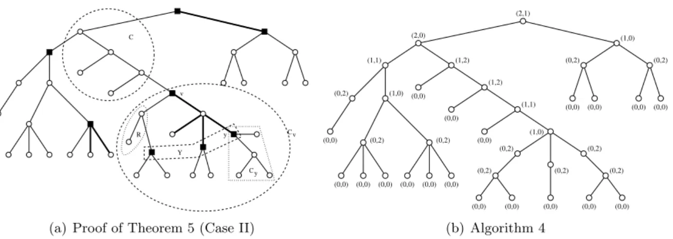
R Y C C y C y v v
(a) Proof of Theorem 5 (Case II)
(2,1) (0,0) (0,0) (0,0) (0,0) (0,0) (0,0) (0,0) (0,0) (0,0) (0,0) (0,0) (0,0) (0,0) (0,0) (0,2) (0,2) (0,2) (0,2) (1,0) (1,1) (2,0) (1,2) (1,2) (1,1) (1,0) (0,2) (0,2) (0,2) (0,2) (1,0) (0,2) (0,0) (0,0) (0,2) (0,0) (0,0) (0,0) (b) Algorithm 4
Figure 1: (Left) Example of notations used in the fourth case of Proof of Theorem 5. The black squares represent searchers, bold edges induce the clear components, Y consists of three occupied nodes,|V(C)|= 5,|V(Cv)|= 16,|V(Cy)|= 5 and|V(R)|= 2. (Right) Example of the labeling computed by ProtocolTwoSearchers (Algorithm 4) of a tree rooted inr.
S0 before step h(S∗) and let X0 be the set of vertices occupied by the searchers at
this step ofS0. At steph(S∗),S0 clears a contaminated componentC ofT\X0. Let
s0 ≥h(S∗) > sbe the first step in S0 when the component C is cleared. Note that,
s0 ≤ N0 since otherwise Protocol InitPos would stop just after step s. According to Lines 15-16 of Protocol InitPos, after the step s,S0 clears the component C by usingκ− |X0|searchers.
Let S0 be the monotone search strategy obtained by modifying S∗ as follows: i)
proceed as the firstssteps inS0 (that are also the firstssteps inS∗ sinces <h(S∗)),
ii) apply all the steps from s+ 1 to s0 in S0 that clear C and perform the greedy moves consisting of removing all the searchers from the vertices in C and from the vertices of X0 with only clear neighbors, iii) proceed according to S∗ after its step
h(S∗) by avoiding all the moves concerningC (placing/removing a searcher on/from
a vertex ofC).
Note that the phase iii) above is possible. Indeed, lets00 be the last step ofS0 before phase iii). After step s00 of S0, when a move is performed inS0, there are at least as
many free searchers as when the corresponding step is done isS∗, in other words the
corresponding move can be performed inS0 usingκ searchers. Finally, to get the contradiction, note thath(S0)> s0 ≥h(S∗).
Case II. h(S∗) > N0, in other words h(S∗) = N0+ 1. Since by our assumption, S0 does not clear T, we have h(S∗) ≤ |S∗|. That is, after step h(S∗)−1 of S0, there are no possible greedy moves and no contaminated components of T \X0 can be cleared using κ− |X0|
searchers. In other words, after this step, the algorithm cannot continue withκ searchers while the tree is not yet clear (Lines 19-20). BothS0 and S∗ have the same configuration
after step h(S∗)−1. Let X0 be the set of vertices occupied by a searcher at this step.
Considering S∗, we show that, after step h(S∗)−1, there is a contaminated component
C of T \X0 such that s(C) ≤κ− |X0|. This will obviously be in contradiction with the assumption that the algorithm cannot continue withκ searchers after stepN0 inS0. LetCbe the first connected component among all the connected components of the contam-inated part ofT\X0 which becomes totally clear by the search strategyS∗, and let s≥N0+ 1
be the step ofS∗ when all the vertices ofC are clear. We claim that at any step of S∗ between
h(S∗) ands, at least|X0|searchers are occupying the vertices ofT\C. In other words, at each
intermediate step inS∗ betweenN0 ands, there are at mostκ− |X0|free searchers. This clearly implies thats(C)≤κ− |X0|, and proves the existence of C as stated above.
To show this claim, we proceed as follows. For any vertexv∈X0, letev ={v, u}be the edge incident tov which lies on the path which connectv to C inT (possibly,u∈V(C)). LetCv be the connected component ofT\ev that containsv. We prove by induction on|X0∩V(Cv)|that at any step ofS∗ between steps h(S∗) and s, at least |X0 ∩V(Cv)| vertices in Cv are occupied by a searcher. This will clearly imply the claim. Indeed, considering the subset W ⊆X0 of all the occupied vertices at step h(S∗)−1 which are incident by an edge toC, for any v ∈W, at
least|X0∩V(Cv)|searchers must occupy the vertices of Cv at any step betweenh(S∗) =N0+ 1 and s in S∗. Since |X0| = Pv∈W |X0 ∩V(Cv)|, this shows that |X0| searchers must be places on some vertices ofT \C at any step between h(S∗) and s, which is the assertion of the above
claim.
To proceed by the induction, consider first the base case where |X0 ∩V(Cv)| = 1. Since
v has at least two contaminated neighbors (because by assumption no greedy move is possible after stepN0 inS0), there must exist a connected componentR 6=C of the contaminated part ofT\X0 such thatR⊆Cv, and such thatR has an edge incident tov. SinceC is cleared before
Rand the strategy is monotone, at any step betweenh(S∗)ands, at least one searcher occupies
a vertex ofR∪ {v} ⊆Cv and this proves the base of induction.
Let us assume now that|X0∩V(Cv)|>1and for any integer strictly smaller than|X0∩V(Cv)| the induction hypothesis holds. This case is depicted in Figure 1(a). Consider the subset
Y ⊆ (X0 ∩V(Cv))\ {v} containing all the vertices y 6= v that are in X0∩V(Cv) such that no other vertex of X0 is on the unique path between y and v. Note that for any y ∈ Y,
|X0∩V(Cy)|<|X0∩V(Cv)|and so, according to the induction hypothesis, at any step between h(S∗)ands, there are at least|X0∩V(Cy)|searchers which occupy some vertices ofCy. Moreover, at least one connected components R 6= C of the contaminated part of T \X0 has an edge incident to v. Note that, by definition of Y, for any y ∈ Y, R∩Cy = ∅. Since C is cleared before R and the strategy is monotone, at any step between h(S∗) and s, at least one searcher
occupies a vertex of R∪ {v} ⊆Cv. This shows that, at any step between h(S∗) and s at least
1 +P y∈Y |X
0∩V(C
y)| = |X0 ∩V(Cv)| searchers must occupy some vertices of Cv, and thus, the induction hypothesis also holds for |X0∩V(Cv)|, and so the claim follows.
This finishes the proof of the first part of the theorem.
Note that at each execution of the while-loop (Line 5) of the protocol, either at least one vertex is cleared, or one searcher becomes free. Therefore, there are at mostn2executions of this loop. Moreover, each execution of this loop first tests the neighborhood of the occupied nodes at most twice (Lines 8 and 10), and then it tests each contaminated componentS by computing
s(S) (Line 15). Since, these components are disjoint then the sum of their sizes is less than n
and, by Theorem 4, this latter computation is performed in linear time. Hence, each execution of the for-loopof ProtocolInitPos is performed in polynomial time.
3.2 Further notations
We now introduce some extra terminology and notations that will be used in the next sections. Let T be a tree rooted in r ∈ V(T). For any v ∈ V(T), let p(v) denote the parent of v (we set {p(r)} =∅), and let Tv denote the subtree ofT rooted in v. By Tˆv we denote the subtree induced by V(Tv)∪ {p(v)}. For any subset X ⊆V(Tv)\ {v} with the property that no vertex of X is on the path between v and any other vertex of X, we denote by SX(v) the component of Tv \X that contains v, and denote by CX(v) (resp., CˆX(v)) the subtree of Tv induced by
v X r=p(v) (a)T v (b) Tv v (c) CX(v) v p(v) (d) CˆX(v) Figure 2: Notations.
V(SX(v))∪X (resp., V(SX(v))∪X∪ {p(v)}) (see Figure 2). In other words,CX(v) is obtained fromTv by removing all vertices that have an ancestor inX.
For any subset I ⊆V(T)and anyv∈V(T)\I, the subsetX(v, I)⊆I denotes the set of all descendantsuofv that are inI with the property that no internal vertices of the path between
u and v belong toI. Finally, let us assume some vertices of a treeT are labeled with integers in{0,· · ·, q}, and a vertexv∈V(T) is not labeled. For any0≤i≤q, to simplify the notation, we denote byX(v, i)the subset X(v, Ii)⊆Ii where hereIi is the set of all labeled vertices of T with label larger or equal toi.
A caterpillar K is a tree that has a dominating path. That is, there is a pathP inK such that any vertex inV(K) either belongs toV(P) or has a neighbor in V(P).
4
To clear a tree by performing one query
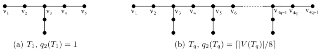
The purpose of this section is to design an algorithm, called OneQuery, that computes s1(T), the smallest number of searchers required to clear a tree T when at most one query can be performed. AlgorithmOneQueryuses, as a black box, AlgorithmTwoSearchers(whose design is postponed to Section 6) which computes q2(T) the smallest number of queries required to clear a given tree T with two searchers.
Note that by Proposition 1, a one-limited search strategy, i.e., a search strategy with one allowed query, consists of the following three basic steps
(1) placing searchers on every vertex inX⊆V(G), with|X| ≤s1(G),
(2) performing the query to locate the contaminated part C of the graph, and
(3) clearing the contaminated componentCby starting from the vertices ofXthat are adjacent to C and by using s1(G) searchers.
More formally, for any treeT and anyk≥1,s1(T)≤k if and only if there exists a subsetX⊆
V(T) such that|X| ≤k, and for any connected componentC of T\X we haves0{Y}(C0)≤k whereY is the set of vertices in X that are adjacent to a vertex in C and C0 is the connected component of T induced byC∪Y.
We prove that for any treeT, ProtocolOneQuerydescribed in Algorithm 2 computess1(T), and a corresponding strategy, in polynomial time. Note that, inOneQuerywe first use Algorithm
TwoSearchers to test ifs1(T) = 2 by checking ifq2(T) = 1.
Once this has been done, given an integer k ≥1, the aim of Protocol OneQuery will be to find a subsetX ⊆V(T)such that the connected components ofT\Xcan be cleared in the way described above, and such that in addition, these components are as large as possible. Performing
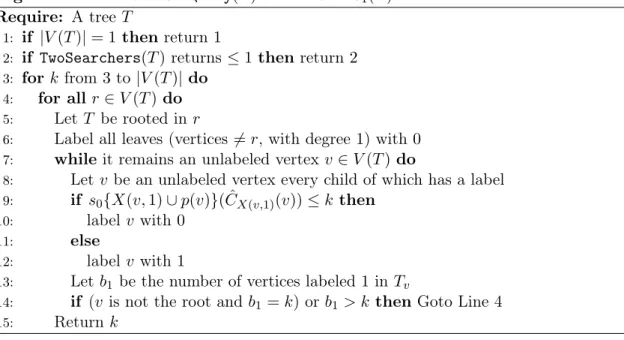
Algorithm 2Protocol OneQuery(T)that returns s1(T) Require: A tree T
1: if |V(T)|= 1 thenreturn 1
2: if TwoSearchers(T) returns≤1thenreturn 2
3: forkfrom 3to |V(T)|do
4: for all r∈V(T) do
5: LetT be rooted inr
6: Label all leaves (vertices 6=r, with degree1) with0
7: whileit remains an unlabeled vertex v∈V(T) do
8: Let v be an unlabeled vertex every child of which has a label
9: if s0{X(v,1)∪p(v)}( ˆCX(v,1)(v))≤kthen
10: labelv with0
11: else
12: labelv with1
13: Let b1 be the number of vertices labeled 1inTv
14: if (v is not the root and b1=k) orb1 > k thenGoto Line 4
15: Return k
in such a way allows to minimize the size of X. If such a subset X of size |X| ≤ k exists, we infer thats1(G)≤k(otherwise,s1(G)> k). Roughly speaking, Protocol OneQueryproceeds as follows. Letk≥1be a fixed integer, and letT be rooted inr ∈V(T). ProtocolOneQuerylabels the vertices ofT with labels0 and1 by starting from the leaves and by proceeding towards the root. At the end of this labeling procedure, the subset X⊆V(T), that we are looking for, will consist of those vertices which are assigned label1. Therefore, if at mostkvertices are labeled1, a one-limited strategy starts by placing the searchers on these vertices and performing a query. The way the labeling procedure has been performed ensures that for any maximal (with respect to inclusion order) connected subsetCof vertices labeled 0, and forY the set of vertices adjacent toC and labeled 1, we haves0{Y}(C∪Y)≤k. Therefore, if ProtocolOneQueryreturnsk, then
s1(T)≤k.
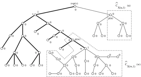
The details of the labeling procedure are as follows and depicted in Figure 3. The procedure is done forT rooted inr for any possible rootr∈V(T) (Line 4). A vertex v∈V(T)is labeled once all its children are assigned a label. X(v,1)is defined as the set of descendantsuofv that are labeled with1, and such that the internal vertices of the path between uand v are labeled
0. (The notations are the same as in Section 3.2.) Knowing that a searcher has to be placed on each vertex ofX(v,1) before the first query (see the discussion in the previous paragraph), Protocol OneQuerytests whether it is necessary to place a searcher on v or not. The answer is yes if and only if by not placing a searcher onv before the query, the component which contains
v and X(v,1), and has internal nodes of label 0, creates a connected component that cannot be cleared with at most ksearchers by starting from the position of the searchers just after the query, i.e. at its border. That is, under the (testing) assumption that a searcher is not placed on
v, this connected component containsCˆX(v), and ProtocolOneQuerytests whether ksearchers starting from X(v,1)∪ {p(v)} can clear CˆX(v,1)(v). v is labeled 0 if this is the case, and it is labeled 1otherwise.
We notice that Lines 13-14 can be replaced by “If more than k vertices are labeled 1 Goto Line 4” without modifying the result achieved by Protocol OneQuery. However, we have pre-sented ProtocolOneQueryin this way to make it fully equivalent to ProtocolApprox(forq= 1) described in Section 5 (see Lemma 1).
0 (u) X(u,1) C (w) X(w,1) C 0 0 0 0 0 0 0 0 0 0 0 0 0 0 0 0 0 0 0 0 0 0 0 0 0 0 0 0 0 1 0 0 0 0 0 0 0 0 0 0 0 0 0 w v r=p(v) 0 p(w) p(u) u 1
Figure 3: Result of Algorithm 2 on T rooted in r and k = 3. Bold edges are the edges of
ˆ
CX(v,1)(v).
k = 3. During this execution, X(u,1) =∅ and u is labeled with 0 because CˆX(u,1)(u) (with 4 nodes) can be cleared starting from X(u,1)∪ {p(u)}={p(u)}using no query with3searchers. Similarly X(w,1) = ∅ since there are no descendants of w labeled with 1, however w must be labeled1because it is not possible to clearCˆX(w,1)(w)starting fromX(w,1)∪ {p(w)}={p(w)}, using no query and 3 searchers. To see this, it is sufficient to see that, first a searcher can be placed onwand the one atp(w)is then removed. Then, the searcher atwcannot be freed while two of its branches (components ofTw\{w}) are cleared. Finally, since two of its branches are not caterpillar, the two remaining searchers cannot clear them without any query. The last example we describe is the one when labelingv. X(v,1) ={w}and CˆX(v,1)(v) is the subtree induced by the bold edges. Again, it is easy to check thatCˆX(v,1)(v) cannot be cleared without query, using three searchers and starting from X(v,1)∪ {p(v)} = {w, p(v)}. Therefore, v receives label 1. Finally, s1(T)≤3 and a strategy consists of placing two searchers onv andw, performing the query and clearing the remaining contaminated component with 3 searchers, starting from v
and w.
Theorem 6. For any tree T, Protocol OneQuery(T) computes s1(T) and a corresponding
one-limited strategy in polynomial time.
Proof. The result clearly holds if s1(T) ≤2 by Lines 1-2 and by Theorem 9 (Section 6). In the following, we assume s1(T)≥3. Let k≥3 be the integer returned byOneQuery(T). Let T be rooted in the vertex which gives the output of the algorithm. As we said before, the strategy consists in placing the searchers on the vertices labeled 1, and performing the query. Then, the connected componentC that remains contaminated can be cleared withksearchers by starting from the vertices labeled 1 in the border ofC (Lines 9-10). Thus, certainlys1(T)≤kholds.
To prove the equality, let S be a monotone one-limited search strategy for clearing T that uses at mostk >2searchers. By Proposition 1, we may assume that the first steps in S consist of placing at mostksearchers on the vertices of a subsetI ⊆V(T)(I 6=∅), and then performing the query. We consider the labeling of the vertices of T obtained by OneQuery(T) (Lines 5-12) whenT is rooted in a vertexr∈I. For any vertexv∈V(T), define jv=|I∩V(Tv)|. We prove by induction on jv that there are at mostjv vertices labeled1inTv. Sincejv < k for anyv6=r (becauser∈I) andjr=|I∩V(Tr)|=|I| ≤k, this proves that after the execution of Lines 5-12 (for the vertex v, when T is rooted in r), since b1 ≤ jv, Line 14 is not executed, there is no return to Line 4. Hence, the output ofOneQuery(T) is at mostk, and this finishes the proof of
our theorem.
To prove the base of our induction, let v be a vertex with jv = 0. Obviously, since S is monotone and there is no recontamination, for anyw∈V(Tv), one can derive fromS a strategy
Sw that clears Tˆw = Tw ∪ {p(w)} by starting from p(w) and by using at most k searchers, without performing any query. In other words, s0{p(w)}( ˆTw) ≤ k. Thus, by the definition of our labeling procedure (Lines 9-10), all vertices of Tv are labeled 0.
Consider now a vertex v with jv > 0, and suppose that for any u with ju < jv the claim holds. We divide the proof into two parts depending on whetherv∈I or not.
Ifv∈I, the result can be easily obtained by applying the induction hypothesis to the children of v. Indeed, since v ∈I, for any child u of v, we haveju < jv, and thus, by the hypothesis of our induction, there are at most ju = |I ∩Tu| vertices labeled 1 in Tu. This shows that there are at most P
uju = |I ∩Tv| −1 vertices labeled 1 in Tv \ {v}, where the sum is over all the children ofv. We infer that there are at mostjv =|I ∩Tv|vertices labeled1 inTv.
Now, suppose that v /∈ I. Let X(v, I) = {v1,· · ·, v`} (`≥ 1) be the set of all descendants
u of v that belong to I, and such that there is no other vertex ofI on the path between v and
u (the notations are the same as in Section 3.2). For any i≤ `and any child z of vi, we have
jz < jv and the induction hypothesis holds for z. That is, for any i≤` and any child z of vi, there are at mostjz vertices labeled1 inTz.
Consider a vertex w ∈ CX(v) that does not lie on any path between v and vi for any i ≤ `. Obviously, for such a vertex we must have jw = 0. By the base of our induction, all vertices in
Tw are labeled0. In other words, this shows that any vertex ofCX(v)which is labeled1 has to belong to a path betweenvandvi for some value of1≤i≤`. For anyi≤`, letui be the vertex (if any) of the unique path between vi and v, including vi andv, that is labeled1 and which is closest tovi. LetU be the set of all the verticesui,1≤i≤`. It is clear that|U| ≤`=|X(v, I)|. We claim there is no other vertex of CX(v)\U with label 1. For the sake of a contradiction, suppose this is not the case and letwbe a vertex ofCX(v)\U which is assigned label1by Lines 6-12 of Protocol OneQuery(T). Let U0 = X(w, U), the set of descendants u of w which belong to U and verify the property that there is no other vertex of U on the unique path between w
and u. By the definition of U, CˆU0(w) is a subtree of CˆX(v). In addition, since U0 ⊂ U and
S is monotone, one can easily derive from S a strategy for clearing CˆU0(w) which starts from
{p(w)} ∪U0 and uses at most k searchers, and which does not perform any query. This shows that s0{{p(w)} ∪U0}( ˆCU0(w)) ≤ k, and by the definition of the labeling scheme (Lines 9-10), the label assigned towis0, a contradiction. We infer that there are at most|U| ≤ |X(v, I)|=`
vertices in CX(v)which are labeled 1.
To conclude, the number of vertices labeled 1 in Tv is bounded above by `+ P
zjz =
`+P
z|Tz ∩I| = |Tv ∩I| = jv. Here, in the sums, z runs over all the children of a vertex
vi ∈X(v, I), for1≤i≤`. The fact thatOneQueryperforms in polynomial time directly follows from Theorem 5.
5
A polynomial time algorithm for
rs
qin trees
This section is devoted to presenting Protocol Approx, formally described in Algorithm 3, that computesrsq(T) in polynomial time for any treeT and anyq >0. Combined with Theorem 3, this leads to a polynomial time2-approximation algorithm for computing sq in trees.
We start by characterizing the family of all trees with restricted q-limited search number two. This will be later used in the design of our algorithms. Recall that the heightof a tree T
is the smallest integer h such that there exist two vertices u, v ∈V(T) called the centers of T, so that either u=v, or uand vare adjacent, and such that any vertexw∈V(T)is at distance
strictly smaller than h from u or v. A tree is called q-simple if it is obtained from any tree S
of height at most q by attaching to any w ∈ V(S) an arbitrary number of paths of arbitrary length.
Theorem 7. Let T be a tree. Then rsq(T) = 2 iff T isq-simple and |V(T)|>1. Furthermore,
this can be decided in linear time.
Proof. Let T be q-simple with |V(T)| > 1. Since |V(T)| > 1, rsq(T) > 1. Let S be a tree of height at most q from which T is obtained by the addition of some paths. We describe a strategy for clearing T using two searchers and at most q queries. Place the two searchers on the center(s) of S and perform the first query. Then, after each query, remove the searcher in the clear component and place it on the neighbor of the other searcher in the contaminated component and perform the next query. By definition of the height, when the last query has been performed, the contaminated part of the tree (if not empty) is a path an end of which is occupied by a searcher. The capture of the fugitive follows easily. Hence,rsq(T) = 2.
By the definition of restricted non-deterministic graph searching and by Corollary 1, for any restricted strategy using two searchers, the set of vertices that have been occupied by the searchers until the jth query must induce a path withj vertices. The result follows easily.
Clearly, one can decide whether a tree is q-simple in linear time.
5.1 Good decomposition of a labeled tree
Given a subtree S of a tree T, define theborder ∂T(S) of S inT as the set of all vertices of S that are adjacent inT to some vertices inT \S.
Let T be a labeled tree in which each vertex has a label in{0,1, . . . , q}. For any0≤`≤q, define the (unique) familyF` of subtrees (possibly reduced to one edge) of level `as the family of all the (inclusion) maximal subtreesS ofT with the property that all the internal nodes ofS
have a label smaller or equal to`. Note that such a maximal subtree can be reduced to an edge with vertices labeled > `.
The following easy remarks are in order. First, note thatFq={T}. Let`∈ {0,· · ·, q−1}. By definition, for any subtree of level`,S ∈ F`, any internal vertex ofS has a label ≤`, therefore, the border of S, ∂T(S), is simply the set of all leaves of S that have a label at least equal to
`+ 1. Moreover, it is clear that the union of all the elements ofF`coversT, and any two distinct subtrees S, S0 ∈ F` intersect in at most one vertexv ∈∂T(S)∩∂T(S0) (in particular, the label of vis at least `+ 1).
Definition 1. The collection {F0,· · ·,Fq} is a k-good decomposition of T if it satisfies the following two properties.
(I) For any 0 < `≤ q, any subtreeS ∈ F` contains at most k vertices with label at least `, and
(II) for any subtree S∈ F0, we have s0{∂T(S)}(S)≤k.
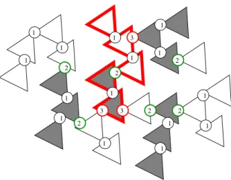
Figure 4 illustrates a 4-good-decomposition of a treeT. In Figure 4, a triangle represents a subtree, a circle is the common vertex between two adjacent triangles and it is a leaf in both corresponding subtrees. The integer in a circle is the label of the corresponding vertex and any vertex not depicted by a circle is labeled with 0. F0 is the set of triangles, i.e., each triangle is a subtree that can be cleared without query by 4 searchers starting from its (at most three) leaves depicted by circles. F3 ={T}. The family F2 is represented by the width of the border of the triangles (red bold or black thin): two adjacent triangles with the same border-width belong to the same subtree of F2. |F2|= 4. The family F1 is represented by the colors (gray
2 1 1 2 1 1 1 1 1 1 2 1 1 2 1 1 2 1 2 3 3 1 3 1
Figure 4: Shape of a 4-good-decomposition of a treeT. F3 ={T},|F2|= 4 and |F1|= 10
or white) of triangles: two adjacent triangles with the same color belong to the same subtree of
F1. |F1|= 10.
The significance of the above definition is given by the following proposition.
Proposition 3. If a tree T with labels in {0,· · ·, q} gives rise to a k-good decomposition {F0,· · ·,Fq}, then rsq(T)≤k.
Proof. The strategy consists in placing first the searchers on vertices labeled by q (at most k
by Property (I) of Definition 1, for T ∈ Fq), and then performing the first query. Proceeding by induction, for any1≤`≤q, once the`th query has been performed, the contaminated part consists of a subtreeSq−` ∈ Fq−` such that
(1) the vertices in ∂T(Sq−`) are all occupied by a searcher (by definition, they have label at leastq−`+ 1), and
(2) no other vertex in S\∂T(S) is occupied by a searcher (since they all have label at most
q−`).
All those searchers that occupy a vertex in V(T \Sq−`) are removed, and then placed on the set L of vertices in Sq−` which are labeled q−`. By Property (I) in Definition 1, at most k searchers can occupy all the vertices in|L∪∂T(S)| ≤k, so this is possible. The(`+ 1)th query is then performed next. Once the qth query has been performed, by Property (II) of Definition 1, the remaining contaminated part S0 ∈ F0 can be cleared starting from ∂T(S0) with at most k searchers (since s0{∂T(S0)}(S0)≤k). This proves the proposition.
In what follows next, we will prove that if Protocol Approx(T, q) returns an integer k ≥3, then the labeling which results from its execution gives rise to a k-good decomposition ofT.
5.2 General description of Protocol Approx.
The general scheme ofApproxis as follows. ProtocolApproxstarts by checking first whether
rsq(T)∈ {1,2}(Lines 1-2). This can be done by Theorem 7.
Then, fixing an integer k≥3, Protocol Approxaims at computing the smallest number q˜≥ 0
such that there exists a subset X ⊆ V(T), with |X| ≤ k, and such that for any connected componentCofT\X, there is a restricted(˜q−1)-limited strategy with the following constraint: LetY be the set of vertices in Xthat are adjacent to a vertex inC, and letC0 be the connected
Algorithm 3Protocol Approx(T, q) that returnsrsq(T),q >0 Require: A tree T
1: if |V(T)|= 1 thenreturn 1
2: if T isq-simplethenreturn 2
3: forkfrom 3to |V(T)|do
4: for all r∈V(T) do
5: LetT be rooted inr and all its vertices be unlabeled
6: Label all leaves (vertices 6=r, with degree1) with0
7: whileit remains an unlabeled vertex v∈V(T) do
8: Let v be an unlabeled vertex every child of which has a label
9: Let bj be the number of vertices labeled≥j inCX(v,j+1)(v),1≤j ≤q
10: if ∃j >0,bj > k then
11: Letm be the greatest integer such thatbm ≥k
12: Labelv withm+ 1
13: else if v is not the root and (∃j >0,bj =kor |X(v, j)|=k−1) then
14: Letm be the greatest integer such thatbm =kor |X(v, m)|=k−1
15: Labelv withm+ 1
16: else if s0{X(v,1)∪ {p(v)}}( ˆCX(v,1)(v))≤k then
17: Labelv with0
18: else
19: Letk0 =kif v is the root and k0 =k−1 otherwise;
20: Letm >0 be the smallest integer such thatbm < k0
21: labelv withm
22: if a vertex is labeled larger thanq thenGoto Line 4
23: // test another root if possible and increase kby one otherwise
24: return k
component of T induced by C∪Y. Then the strategy uses k searchers for clearing C0, and starts by placing the searchers on the vertices of a superset ofY and performing the first query. If at some step of the algorithm q˜becomes larger than q, the allowed number of queries, then
Approx increasesk by one and restart the whole procedure. The way this is done is similar to ProtocolOneQuery: ProtocolApproxaims at finding a subsetX⊆V(T)such that the connected components ofT\Xcan be cleared in the way described above, and such that these components are as large as possible.
More precisely, the aim of ProtocolApprox(T, q)is to produce a labeling of all the vertices of
T with labels in{0,· · ·, q}giving rise to ak-good decomposition{F0,· · ·,Fq}forT, and for the smallest value of k, such that in addition the subtrees inF0 are as large as possible. Once such a labeling has been found, Proposition 3 (and its proof) shows that rsq(T)≤k and produces a strategy for clearing ofT. The proof of the reverse inequality, yielding to the equality ofrsq(T) with the output of the algorithm, is similar to the proof of Theorem 6 in the case q = 1. We show that rsq(T)≥k by induction onq and next Lemma serves as basis of the induction. Lemma 1. For q= 1 Protocol Approx proceeds as OneQuery (Algorithm 2).
Proof. If|V(T)|= 1or T is1-simple, clearly both algorithms achieve the same result.
The only difference between both algorithms is that Protocol OneQuery labels the vertices only with 0 or 1, and stops if at some step, strictly more than k vertices have received label
1, while Protocol Approx increases the label used, i.e., it uses the label 2, when more than k
vertices have received the label 1. But, at this step, Line 22 of Approx stops the execution as well.
More formally, consider an execution of bothOneQuery(T)andApprox(T,1)whenTis rooted in some r ∈V(T)and for some given k. Suppose that the vertex v∈V(T) is the vertex which is going to be labeled, and assume that all the vertices inV(Tv)\ {v} have already received the same labels by both algorithms.
To avoid confusion, note that the variable b1 used by Approx(T,1)is the number of vertices labeled with 1inTv before labeling v (i.e., the number of vertices labeled with 1inTv without consideringv) while the variableb1 used byOneQuery(T) is the number of vertices labeled with
1 inTv after labelingv (considering v).
If ProtocolApprox(T,1)executes Line 12, i.e., the number of vertices labeled1inTv\ {v}is strictly larger thank, then v is labeled with 2and Line 22 will initiate another execution (with another root, or by increasingkby one). But in this case, after labeling the vertex precedingv, Line 14 of OneQuerywill also do the same.
If Approx(T,1)executes Line 15, again Line 22 will initiate another execution. In this case,
vis not the root. Moreover, either strictly larger than kvertices are labeled1inTv and Line 14 of OneQuery will do the same. Or |X(v,1)| = k −1. But in this case, by Proposition 2,
s0{X(v,1)∪ {p(v)}}( ˆCX(v,1)(v))> k, and Line 12 ofOneQuerylabels vwith1, and thenb1 =k (Line 13 ofOneQuery). In the latter case, again, Line 14 ofOneQueryinitiates another execution. Hence, we may assume that Line 16 of ProtocolApproxand Line 9 of ProtocolOneQueryare executed, which perform the same test.
If v is labeled with 0 by both algorithms, then Protocol Approx will try to label the next vertex. On the other side, OneQuery does the same. Indeed, for the sake of a contradiction, suppose instead,OneQueryinitiates another execution. This means either,b1 > k, or,b1 =k, and
vis not the root. But, sincevis labeled0, the variableb1considered at Line 13 ofOneQueryhas the same value as the variableb1 considered at Line 9 ofApprox(T,1). This meansApprox(T,1) should have executed Line 12 or Line 15, which is clearly a contradiction.
Finally, let us assume thatvis not labeled0, and hence, it is labeled1byOneQuery. Suppose first thatApproxlabelsvwith an integer strictly larger than1. This being the case, Line 22 will initiate another execution. In this case, it is easy to check that OneQuerywill execute Line 14, i.e., initiate another execution. In the only remaining case, suppose that Approx labels v with
1. Then it tries to label the next vertex or stops ifv is the root. This means that the variableb1 ofApproxis strictly smaller thank0 wherek0 =kif vis the root, andk0 =k−1otherwise. But then, the variable b1 of OneQuery is smaller or equal to k0, and thus, OneQuery does the same asApprox. This finishes the proof of the lemma.
The following lemma is straightforward from the definition of Protocol Approx.
Lemma 2. Let T be a tree and q > q0 ≥ 1. Suppose that Approx(T, q0) returns k¯ during an execution when T is rooted in r. Then, when k = ¯k and T is rooted in r, the two labelings obtained by Lines 5-21 of Approx(T, q) andApprox(T, q0) are identical.
5.3 Main Theorem.
We can now state and prove the main theorem of this paper.
Theorem 8. For any tree T and any integer q > 0, Approx(T, q) computes rsq(T) and a
corresponding restricted q-limited search strategy in time polynomial in |V(T)| (independent of
q).
The rest of this section is devoted to the proof of the above theorem. Let k¯ be the integer returned byApprox(T, q). To prove the theorem, we show that both the inequalitiesrsq(T)≤¯k and rsq(T)≥k¯ hold.
Proof of the inequality rsq(T)≤¯k. First note that if rsq(T) ∈ {1,2} (Lines 1-2), the result is valid by Theorem 7. Let us assume that Approx(T) returns an integerk¯≥3, and letr ∈V(T)
be the root during the iteration that returns k¯. We prove that the resulted labeling gives rise to ak¯-good decomposition ofT. Hence, the inequalityrsq(T)≤k¯ follows from Proposition 3. To prove this, first note that, by Line 22 of Approx(T), all vertices have received a label ≤q. Let {F0,· · ·,Fq} be the collection of families of subtrees ofT defined in Section 5.1. We show that both the properties (I) and (II) in Definition 1 are satisfied.
Consider the base case`=q. Recall thatFq ={T}. For the sake of a contradiction, suppose that more than ¯kvertices are labeled with q. Consider the last execution of the while-loop, i.e., the one which assigns a label tor. If more thank¯vertices distinct fromrare labeled withq, then at this step we have bq >¯k(Line 10) and r has to be labeled with an integer p > q (Line 12), which is a contradiction. Therefore, beforer being assigned a label, we must have bq = ¯k, and
r will be labeled either0 (Line 17) or p 6=q (Lines 20-21). This means that exactly ¯kvertices are labeled with q, which is again a contradiction. Therefore, (I) holds for`=q.
Let 0≤` < q and letS ∈ F`. Let v∈V(S) be the vertex of S which is labeled last, i.e.,S is a subtree of Tv. Note that S=CX(v,`+1)(v). There are two cases to consider:
• Either, v is labeled with an integer ≥`+ 1. Then,v has to be a leaf of S. Letu be the child of v that belongs toS. If the label of uis at least`+ 1, thenV(S) ={u, v} and (I) holds.
So let us assume that u is labeled with an integer ≤`. If`= 0, Line 16 of Approx (when labelingu) ensures that (II) is valid. Thus, we may assume thatuis labeled with a strictly positive integer.
For the sake of a contradiction, let us assume that at least ¯k vertices of S \ {v} = CX(u,`+1)(u) have a label at least `. If at least ¯k vertices ofS\ {v, u} were labeled with an integer≥`, or if|X(u, `)|= ¯k−1, then uwould have been assigned a label≥`+ 1by Lines 12 or 15, which is not the case. This shows that(¯k−1)vertices ofS\ {v, u} have a label≥` and the label ofu has to be at least `, i.e., exactly `by the previous discussion. However, in this case, Lines 20-21 label u (which is not the root) with m6=`, which is a contradiction.
• Or,v is labeled with an integer≤`. By the definition ofS ∈ F`,vis the root ofT. Letb` be the number of vertices labeled at least`inS\ {v}=CX(v,`+1)(v)\ {v} before labeling
v. If b`> k, thenvis labeled at least`+ 1 by Line 12 which is not the case. Thus,b`≤k¯. Ifb` <k¯, then obviously the number of vertices of label ≥` inS is at most k¯. If b` = ¯k, then by Line 21,vreceives a labelm6=`, and by our assumptionm≤`. This shows again that at most¯kvertices are labeled with an integer≥`inS.
We have proved that {F0,· · ·,Fq} is a ¯k-good decomposition, and by Proposition 3, rsq(T) ≤
¯ k.
Proof of the inequality rsq(T)≥¯k. We now prove that the converse inequality holds. LetS be a monotoneq-limited search strategy forT that usesκsearchers. We prove below that Protocol
Approx(T, q) returns at most κ. We do this by showing that for the value of k = κ, and for some vertexrofT (that we will designate below), the labeling procedure described in Lines 5-21 of Protocol Approx(T, q) produces a labeling which does not contain any vertex of label > q. This shows that the integer ¯kreturned by Approx(T, q) is at mostκ, which implies the desired inequality.
To do so, since we are going to proceed by induction, we need to consider a more general version of restricted graph searching (and ProtocolApprox(T, q)), in which we impose that some leaves
of the tree are occupied by a searcher when the first query is performed. More precisely, let L
be a subset of vertices of degree one inT. Let rsq{L}(T) be the minimum number of searchers needed to restricted monotonously search a tree T with the extra constraint that Lis a subset of the set of occupied vertices when the first query is performed; we say that the strategy starts fromL.
Protocol Approx(T, q,L) is defined by replacing Line 6 ofApprox(T, q) by the following:
“For any leafv ofT (different fromr), ifv∈L, then label v withq, and otherwise, labelvwith
0”.
Note that rsq{∅}(T) =rsq(T), and that Approx(T, q,∅) is identical to Approx(T, q).
In this more general setting, assume again that k¯ is the result of Protocol Approx(T, q,L). We will prove below that¯k≤rsq{L}(T).
Letq ≥1. LetLbe a subset of leaves ofT. LetS be a monotone restricted q-limited search strategy for T that uses κ > 2 searchers and starts from L. Suppose that I ⊆ V(T) is the non-empty subset of vertices such that S first places|I| ≤κsearchers on vertices of I and then performs the first query. Note that, by definition, we have L ⊆ I. Obviously, we can assume that L is the set of all vertices of degree one in I, since otherwise, there is no need to place a searcher on a leaf which does not belong to L (since the first query does not provide any new information depending on whether that leaf belongs toI or not).
Fix a vertex r∈I. Let us consider the labeling of the vertices ofT produced by Lines 5-21 of ProtocolApprox(T, q,L)for the value ofk=κ and whenT is rooted inr. For anyv∈V(T), definejv =|I ∩V(Tv)|
We prove by induction on q≥1 that the following claim holds.
Claim 1. For any v ∈ V(T), there are at most jv vertices labeled with q in Tv, and no vertex
of Tv is labeled with an integer strictly larger thanq.
Clearly, once the claim has been proved, we infer that ProtocolApprox(T, q,L)returnsk¯≤κ, which concludes the proof of the theorem.
To show the above claim in the base case of our induction, q = 1, let us define Protocol
OneQuery(T,L), L being any subset of leaves of T, as the algorithm obtained from Protocol
OneQuery(T) by replacing Line 6 by
“For any leaf v (different fromr) ofT, if v∈L, then labelv with1, and labelv with0
otherwise”.
A direct generalization of the proof of Lemma 2 allows to show thatOneQuery(T,L)achieves the same result asApprox(T,1,L). Moreover, a direct generalization of the proof of Theorem 6 proves
that the execution of
OneQuery(T,L) returns at most κ (in particular, as the proof of that theorem shows, when
T is rooted in r). Hence, the proposition holds forq = 1.
By induction, let us assume that Claim 1 holds for any1≤q0 < q. We proceed by a second induction on the value of jv and show that it also holds for q. Letv be a vertex of T.
In the base case of our (second) induction,jv = 0(hence,v6=r). In this case, one can easily derive a restricted (q−1)-limited strategy S0 from S that clears Tˆv =Tv∪ {p(v)}, wherep(v) is the parent of v, and uses at most κ searchers. In addition, in S0 the first steps consist in placing searchers on a subsetI0,p(v)∈I0, and then performing a query. The subsetI0\ {p(v)} is precisely the set of all occupied vertices in Tv according to the strategy S when the second query is performed, in the case whenTv is still contaminated after the first query (note that this can happen precisely becauseI∩Tv =∅). This in particular shows that rsq−1( ˆTv)≤κ. By our