Development of Backtracking Search Optimization Algorithm Toolkit in LabVIEW™

(1)

Procedia Computer Science 57 ( 2015 ) 241 – 248

Peer-review under responsibility of organizing committee of the 3rd International Conference on Recent Trends in Computing 2015 (ICRTC-2015) doi: 10.1016/j.procs.2015.07.476

ScienceDirect

3rd International Conference on Recent Trends in Computing 2015 (ICRTC-2015)

Development of Backtracking Search Optimization Algorithm

Toolkit in LabVIEW

™

Yashpal Sheoran

1,

*, Vineet Kumar

2

, K.P.S. Rana

3

, Puneet Mishra

4

, Jitendra Kumar

5

and Sreejith S. Nair

6

Division of Instrumentation and Control Engineering, Netaji Subhash Institute of Technology, Sector-3, Dwarka,New Delhi-110078,India

Abstract

In this paper a Backtracking Search Optimization Algorithm (BSA) toolkit has been developed in the LabVIEW™ environment. LabVIEW™ provides a graphical programming environment to design measurement and control applications. The development of BSA toolkit was motivated by the fact that only Differential Evolution (DE) toolkit was provided in LabVIEW™. Thus to design BSA toolkit, several modular virtual instruments have been developed for each BSA process. Developed BSA toolkit has been tested on several benchmark test functions and a comparative study with inbuilt DE toolkit has been performed, which shows results obtained from BSA toolkit are found superior to DE toolkit.

Peer-review under responsibility of the organizing committee of the 3rd International Conference on Recent Trends in Computing 2015 (ICRTC-2015).

Keywords: Backtracking Search Optimization Algorithm; Optimization; Optimization Techniques; Evolutionary Algorithms; Virtual Instruments.

1.Introduction

Optimization is a very important aspect of engineering problems such as digital signal processing applications [1], mechanical design problems [2], image processing applications [3], and many others. The main aim of optimization algorithms is to find the global optimum of an optimization problem by systematically choosing input values within some constrains. An optimization problem may have a complex, non-linear or non-differential form. It is desired for an optimization algorithm to reach global minimum as quickly as possible irrespective of the nature of the optimization problem [4].

The optimization technique can be categorized as: conventional optimization techniques and Meta-heuristics optimization techniques. Conventional optimization techniques guarantee to find global minimum but they are

* Corresponding author. Tel.: +91-828-528-7203; fax: +91-11-25099022.

E-mail address: [email protected]

Peer-review under responsibility of organizing committee of the 3rd International Conference on Recent Trends in Computing 2015 (ICRTC-2015)

(2)

problem specific, while Meta-heuristics optimization techniques are not problem specific rather generic but they may not guarantee to find global minimum for a problem. Moreover, when objective function is non-linear and non-differentiable Meta-heuristics techniques can provide better results [4].

Meta-heuristics techniques can be further classified into three categories: physics-based, swarm intelligence (SI) and evolutionary algorithms (EAs) [5]. Physics-based optimization techniques are based on physical rules. In physics-based algorithm search agents interact and adjust their values in the search space according to some physical rules like gravitational rules, ray casting rules etc. Some of physics-based algorithms are Big-Bang-Big-Crunch [6], Gravitational Search Algorithm [7], Ray optimization [8], Black Hole [9] etc. The second category is SI techniques, which model the social behaviour of swarms or flocks in nature to find global optimum. Examples of some SI techniques are Particle Swarm Optimization (PSO) [10], Ant Colony Optimization (ACO) [11], Cuckoo Search [12] etc. PSO algorithm models choreographic movements of super organisms such as fish, birds etc., it utilizes the individual experience to find global optimum. While ACO algorithm is based on how ants access their food to find global optimum more effectively.

The third category is EA techniques, which are basically based on the concept of evolution in nature. In EA techniques an initial randomly generated population is evolved to achieve optimization. Each new generation is generated by using process of mutation and crossover. Thereafter selection process ensures that newly generated population have a better fitness than previously generated population, thus EA provides optimized solution. In this regard many bio-inspired EAs have been proposed to solve complex optimization problems. DE is one of the popular EA based algorithm to solve global optimum problems. DE has five mutation strategies and two crossover strategies which enhance its effectiveness [13]. Various derivative version of DE have been proposed such as the self-adaptive differential evolution algorithm [14], the adaptive differential evolution algorithm [15], and the parameter adaptive differential evolution algorithm [16]. Other EA based algorithms are Genetic Algorithm [17], Evolutionary Programming [18], Evolution Strategy [19] etc.

In this paper a toolkit for BSA algorithm has been designed in LabVIEW™ environment. BSA is a more effective EA based technique recently proposed by Civicioglu [4]. The ability of BSA to solve different kinds of optimization problems is more effective than other EA techniques. A BSA algorithm utilizes the previously generated populations for generating a new population generation with better fitness values. This concept mimics the nature of some hunting species which goes back to the hunting areas which were fruitful in the past. Moreover, BSA has a very different mutation strategy with respect to DE; which uses only one directional individual for each target individual. Also BSA has a non-uniform crossover strategy which is more complex in contrast to many genetic algorithms [4, 20].

LabVIEW™ is a software package provided by National Instruments and it is a perfect tool for measurement control, signal processing applications, and prototyping applications. LabVIEW™ software dominates over its counterpart tools because of its compatibility of interfacing with wide variety of hardware [21]. LabVIEW™ 2012 version 12.0 (32-bit) has been used to develop BSA toolkit.

In further sections the paper is organized as follows, in Section II brief overview of BSA has been presented. Details of BSA toolkit design have been discussed in Section III. BSA toolkit has been verified for several benchmark test functions [22] and comparative study with DE toolkit is presented in Section IV. Finally the paper has been concluded.

2.Backtracking Search Optimization Algorithm

BSA is an iterative EA to find global minimum for a problem. It can also find global Maximum of a problem by finding minimum of the inverse of that problem as shown in Eq. 1.

(3)

Where א is a very small value belongs to the range (0.1, 0.01) and f(x) is the given optimization problem. BSA algorithm is briefly explained step by step in the following section.

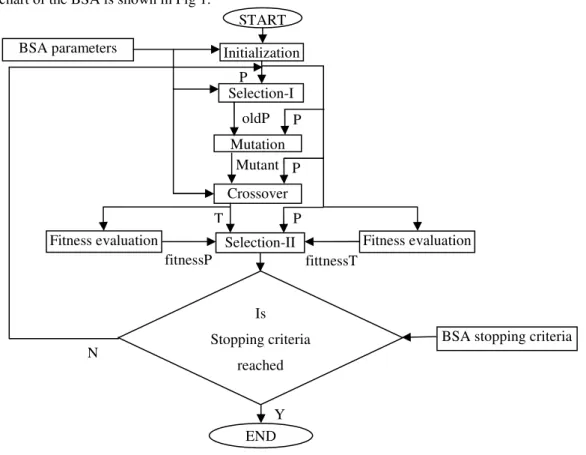
In initialization process individuals of population (P) are generated in a random fashion according to Eq 2. In next process of selection-I, initially individuals of historical population (oldP) are generated by using Eq 3. In second step oldP is updated by using Eq 4. In third step the individuals of oldP are reshuffled randomly. This oldP record has been kept same until it is changed in further iterations. Thus BSA possesses memory [4].

After the process of selection-I, an initial trial population (mutant) is generated by mutation process from P and oldP using Eq 4. In the next process of crossover final trial population (T) is generated using mutant and P. In last process of selection-II P is updated with individuals of T having better fitness. At the end of this process, global minimum and global minimizer values are updated with the best fitness and corresponding individual respectively. These processes except initialization are repeated until the stopping criteria have been reached.

The flow chart of the BSA is shown in Fig 1.

Fig. 1. Flow chart of BSA

3.Development of BSA Toolkit

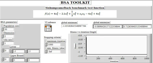
In this section, several VI’s used for designing BSA toolkit have been explained one by one. In BSA toolkit VI, as shown in Fig. 2, various BSA parameters, stopping criteria and VI reference of benchmark test function VI (a separate VI to implement benchmark test functions) are given as input, while global minimum, global minimizer and fitness versus iteration graph are taken as outputs.

Y N fittnessT fitnessP Mutant T P P oldP P P Selection-II Mutation Fitness evaluation Is Stopping criteria reached

BSA stopping criteria

END Crossover Selection-I BSA parameters START Initialization Fitness evaluation

(4)

Fig. 2. BSA.vi 1.1. Initialization.vi

Initialization.vi, as shown in Fig. 3 generates an initial P randomly according to Eq. 2. For i=1, 2, 3… N and j=1, 2, 3… D

Pi,j= rand*(upj-lowj)+lowj (2)

Where N and D are the population size and the problem dimensions respectively, lowj and upj are lower and upper bound respectively, and rand is a random number in the range 0 to 1 generated by using random number generator function in LabVIEW™.

Fig. 3. Initialization.vi

1.2. Selection-I.vi

The oldP is determined from P by Selection-I.vi, as shown in Fig. 4; initially oldP is generated using Eq. 3. For i=1, 2, 3… N and j=1, 2, 3… D

Pi,j= rand*(upj-lowj)+lowj (3)

After oldP is initialized randomly by Eq. 2 for first iteration,it is redefined by P in random manner. For i=1, 2, 3… N (i.e. population size) two uniformly distributed random numbers in the range 0 to 1 are generated. If first number is found to be less than the second number then the ith individual of oldP is replaced by the corresponding individual of P.

Fig. 4. Selection-I.vi

1.3. Mutation.vi

Using mutant.vi, as shown in Fig 5, Mutant is generated as per Eq. 4.

Mutant = P + F ൈ (oldP - P) (4)

Where F=3 ൈrandn, and randn generates a random number in the range [0, 1], with normal distribution [4]. Fig. 5. Mutation.vi BSA parameters P P BSA parameters oldP BSA parameters Stopping criteria VI reference Global minimum Global minimizer Fitness v/s iteration graph

oldP

(5)

1.4. Crossover.vi

T is generated by crossover.vi, as shown in Fig 6, in two successive steps; in the first step, a binary integer matrix map having values either 0 or 1 with dimensions same as P is generated. Initially all the elements of matrix map are assigned as 1 thereafter some of its element are set to 0 by using two predefined random strategies as discussed in [17]. In the second step, initially values of T are assigned equals to Mutant. After that some of the elements of T are updated with the corresponding element of P, if the respective element of map is found to be 1. At last a boundary control mechanism is also used to limit the values of T’s element within the lower and the upper bounds.

Fig. 6. Crossover.vi

1.5. Selection-II.vi

P is updated to yield next generation population with better fitness by selection-II.vi, as shown in Fig 7. The individuals of P are replaced with corresponding individuals of T which have better fitness. Selection-II.vi also updates global minimum and global minimizer with the best obtained fitness and corresponding individual of updated P.

Fig. 7. Selection-II.vi

1.6. Fitness evaluation.vi

Fitness of an array of individuals is evaluated using Fitness evaluation.vi. The VI reference of the benchmark test function and array of individuals are given as input and individual’s Fitness is taken as output, as shown in Fig 8.

Fig. 8. Fitness evaluation.vi

1.7. Display.vi

Display.vi, as shown in Fig 9 is used to run benchmark test function VI for finally obtained optimized parameters. Fig. 9. Display.vi Global minimizer VI refrence fitnessPP T fitnessT Global minimum Global minimizer Updated P MutantP BSA parameters T VI reference Fitness Array of individuals

(6)

4.Experiments and Results

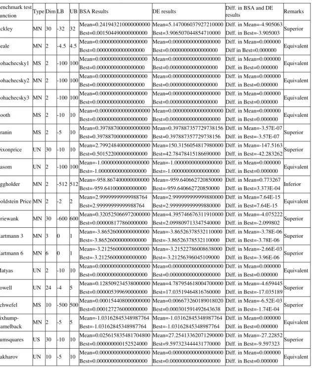
In this section, BSA toolkit has been verified on several benchmark test functions to find the global minimum. Table 1 shows the comparative results of inbuilt DE toolkit and BSA toolkit, along with various constrains of benchmark test functions.

The population size and maximum number of iterations for both the algorithms are set to be 30 and 1000 respectively. Other parameters like dimension, lower and upper bound have been taken according to the benchmark test functions. For BSA toolkit, mix rate is set to 1, while DE toolkit parameters are taken as default as in LabVIEW™.

The stopping criteria to the BSA toolkit is either the specified maximum number of iterations has been reached, or, the objective functions value is lesser than specified minimum fitness value.

The Front Panel and Block Diagram of developed BSA toolkit VI for the Sixhumpcamelback benchmark test function are shown in Fig. 10 and Fig. 11 respectively.

Fig. 10. BSA.vi Front Panel

(7)

Table 1: Results for benchmark test functions (Dim: Dimension, LB: Lower Bound, UB: Upper Bound, M: Multimodal, U: Unimodal, S: separable, N: Non-separable, Diff.: Difference)

Benchmark test

Function Type Dim LB UB BSA Results DE results

Diff. in BSA and DE

results Remarks Ackley MN 30 -32 32 Mean=0.241943210000000000 Best=0.001504490000000000 Mean=5.147006037927210000 Best=3.906507044854710000 Diff. in Mean=-4.905063

Diff. in Best=-3.905003 Superior

Beale MN 2 -4.5 4.5 Mean=0.00000000000000000

Best=0.00000000000000000

Mean=0.00000000000000000 Best=0.00000000000000000

Diff. in Mean=0.000000

Diff in Best=0.000000 Equivalent

Bohachecsky1 MS 2 -100 100Mean=0.00000000000000000

Best=0.00000000000000000

Mean=0.00000000000000000 Best=0.00000000000000000

Diff. in Best=0.000000 Equivalent

Bohachecsky2 MN 2 -100 100Mean=0.00000000000000000

Best=0.00000000000000000

Mean=0.00000000000000000 Best=0.00000000000000000

Bohachecsky3 MN 2 -100 100Mean=0.00000000000000000

Best=0.00000000000000000

Mean=0.00000000000000000 Best=0.00000000000000000

Booth MS 2 -10 10 Mean=0.000000000000000000

Best=0.000000000000000000

Mean=0.000000000000000000 Best=0.000000000000000000

Branin MS 2 -5 10 Mean=0.397887000000000000

Best=0.397887000000000000

Mean=0.397887357729738156 Best=0.397887357729738156

Diff. in Mean=-3.57E-07

Diff. in Best=-3.57E-07 Superior

Dixonprice UN 30 -10 10 Mean=2.799248400000000000

Best=0.501522000000000000

Mean=150.3156054817980000 Best=42.78478415186690000

Diff. in Mean=-147.5163

Diff. in Best=-42.283262Superior

Easom UN 2 -100 100Mean=-1.00000000000000000

Best=-1.00000000000000000

Mean=-1.00000000000000000 Best=-1.00000000000000000

Eggholder MN 2 -512 512Mean=-958.867400000000000

Best=-959.641000000000000

Mean=-959.640662720850000 Best=-959.640662720850000

Diff. in Best=3.373E-04 Inferior

Goldstein Price MN 2 -2 2 Mean=2.99999999999988764

Best=2.99999999999988764

Mean=2.999999999999880000 Best=2.999999999999880000

Diff. in Mean=7.64E-15

Diff. in Best=7.64E-15 Equivalent

Griewank MN 30 -600 600Mean=0.320525066972000000

Best=0.000008177860000000

Mean=4.395746676311910000 Best=2.099809713347540000

Hartmann 3 MN 3 0 1 Mean=-3.86526000000000000

Best=-3.86526000000000000

Mean=-3.86526378532110000 Best=-3.86526378532110000

Hartmann 6 MN 6 0 1 Mean=-3.21256000000000000

Best=-3.21256000000000000

Mean=-3.21522786008638000 Best=-3.21256396045109000

Matyas UN 2 -10 10 Mean=0.000000000000000000

Best=0.000000000000000000

Mean=0.000000000000000000 Best=0.000000000000000000

Powell UN 24 -4 5 Mean=0.128509234538000000

Best=0.000005399690000000

Mean=4.787954618004700000 Best=17.03519464816760000

Diff. in Best=-17.035189Superior

Schwefel MS 10 -500 500Mean=0.000154408000000000

Best=0.000127276000000000

Mean=0.006673260189018020 Best=0.000301591492643638

Sixhump- Camelback MN 2 -5 5 Mean=-1.03162845348987764 Best=-1.03162845348987764 Mean=-1.03162845348987764 Best=-1.03162845348987764 Diff. in Mean=0.000000

Sumsquares US 30 -10 10 Mean=0.025615835481704800

Best=0.000000000152524000

Mean=27.25413362071290000 Best=9.597323444431770000

Zakharov UN 10 -5 10 Mean=0.000000000000000000

Best=0.000000000000000000

Mean=0.000000000000000000 Best=0.000000000000000000

(8)

5.

Conclusion

In this paper an evolutionary algorithm based Backtracking Search Algorithm toolkit has been developed in LabVIEW™ 2012 version 12.0 (32-bit). Backtracking Search Algorithm toolkit is developed using the concept of modular virtual instruments to make it an effective user friendly LabVIEW™ code. The developed Backtracking Search Algorithm toolkit has been tested on various types of benchmark test functions. The comparative study has been performed with the inbuilt Differential Evolution toolkit of the LabVIEW™. For low dimension benchmark test function both Backtracking Search Algorithm toolkit and Differential Evolution toolkit provides equivalent results, but for functions having higher dimension such as Ackley, Dixonprice, Powell etc.; Backtracking Search Algorithm toolkit provides superior result than Differential Evolution toolkit. The developed Backtracking Search Algorithm toolkit can be further utilized in science and engineering field for optimization problems.

References

1. Das S, Kanor A. A swarm intelligence approach to the synthesis of two-dimensional IIR filters. Engineering Applications of Artificial

Intelligence 2007;20:1086-96.

2. He Q, Wang L. An effective co-evolutionary particle swarm optimization for constrained engineering design problems. Engineering

Applications of Artificial Intelligence 2007;20(1):89-99.

3. Falco ID, Cioppa AD, Maisto D, Tarantino E. Differential evolution as a viable tool for satellite image registration. Applied Soft

Computing 2008;8:453-62.

4. Civicioglu P. Backtracking search optimization algorithm for numerical optimization problems. Applied Mathematics and Computation

2013;219:8121-44.

5. Mirjalili S, Mirjalili SM, Lewis A. Grey wolf optimizer. Advances in Engineering Software 2014;69:46-61.

6. Erol OK, Eksin I. A new optimization method: big bang-big crunch. Advances in Engineering Software 2006;37(2):106-11.

7. Rashedi E, Nezamabadi-Pour H, Saryazdi S. GSA: a gravitational search algorithm. Information Sciences 2009;179(13):2232-48.

8. Kaveh A, Khayatazad M. A new meta-heuristic method: ray optimization. Computers and Structures 2012;112:283-94.

9. Hatamlou A. Black hole: a new heuristic optimization approach for data clustering. Information Sciences 2013;222:175-84.

10.Kennedy J, Eberhart R. Particle swarm optimization. IEEE International Conference on Neural Network, Perth, Australia, 27 Nov. -

1Dec, 1995;4:1942-8.

11.Dorigo M, Maniezzo V, Colorni A. Ant system: optimization by a colony of cooperating agents. IEEE Transaction on System Man and

Cybernetics 1996;26(B):29-41.

12.Yang XS, Deb S. Cuckoo search via levy flights. World Congress on Nature and Biologically Inspired Computing, Coimbatore, India,

9- 11Dec, 2009;4:210-4.

13.Storn R, Price K. Differential evolution-a simple and efficient adaptive scheme for global optimization over continuous spaces. Journal

of Global Optimization 1997;11:341-59.

14.Qin AK, Suganthan PN. Self-adaptive differential evolution algorithm for numerical optimization. IEEE Transaction on Evolutionary

Computation 2005;1(3):1785-91.

15.Brest J, Griener S, Boskovic B, Mernik M, Zumer V. Self-adapting control parameters in differential evaluation: a comparative study

on numerical benchmark problems. IEEE Transaction on Evolutionary Computation 2006;10:646-57.

16.Zhang J, Sanderson AC. JADE: adaptive differential evolution with optional external archive. IEEE Transaction on Evolutionary

Computation 2009;13:945-58.

17.Holland JH. Adaptation in natural and artificial systems. 1st_{ed. Massachusetts: MIT Press; 1992.}

18.Yao X, Liu Y, Lin G. Evolutionary programming made faster. IEEE Transaction on Evolutionary Computation 1999;3:82-102.

19.Hansen N, Müller SD, Koumoutsakos P. Reducing the time complexity of the derandomized evolution strategy with covariance matrix

adaptation (CMA-ES). IEEE Transactions on Evolutionary Computation 2003;11:1-18.

20.Civicioglu P. http://www.pinarciviciglu.com/bsa.html, accessed on 23 October, 2014.

21.Travis J, Kring J. LabVIEW for everyone: graphical programming made easy and fun. 3rd_{ed. New Jersey: Prentice-Hall; 2006.}

22.Jamil M, Yang XS. A literature survey of benchmark functions for global optimization problems. International Journal of Mathematical